Considering the Life-Cycle Cost of Distributed Energy-Storage Planning in Distribution Grids


1
Key Laboratory of Smart Grid of Ministry of Education, Tianjin University, Tianjin 300072, China
2
State Grid Beijing Electric Power Research Institute, Beijing 100031, China
*
Author to whom correspondence should be addressed.
Appl. Sci. 2018, 8(12), 2615; https://doi.org/10.3390/app8122615
Submission received: 31 October 2018
/
Revised: 7 December 2018
/
Accepted: 9 December 2018
/
Published: 13 December 2018
(This article belongs to the Special Issue Active Distribution Network)
Abstract
:In the face of the radical revolution of energy systems, there is a gradually held consensus regarding the adoption of distributed renewable energy resources, represented by Photovoltaic (PV) and wind generation. Consequently, the distributed Energy Storage Systems (ESSs) have become increasingly important in the distribution networks, as they provide the arbitrage and ancillary services. Determining the optimal installation site and the capacity of the distributed ESSs will defer the network reinforcements, reduce the investment of ESSs, and improve the reliability, flexibility, and efficiency of distribution grids. In order to investigate the optimal ESS configuration and to solve voltage fluctuations brought by the increased penetration of PV, in this study a two-stage heuristic planning strategy has been proposed, which considers both the economic operation and the lifetime of the distributed ESSs, to determine the optimal sitting and sizing of the ESSs, in the distribution grids. The first stage decides the optimal installation site and the economic scheduling of the ESSs, aiming to minimize the fabricating cost of the distributed ESSs and the network losses. Based on the output of the first stage, the second stage planning is further delivered to achieve the optimal ESS capacity, considering the Life-Cycle Cost (LCC) minimization. Finally, the feasibility and effectiveness of the proposed method is verified on a typical distribution case study network.
1. Introduction
Due to the severe environmental pollution caused by fossil fuels and their depletion, the utilization of distributed renewable energy resources has been considered to be a practical approach to address the supply–demand stress, and to reduce the anthropogenic greenhouse gas emissions. However, the intermittent impacts, brought about by the renewable resources, requires significant reinforcement for the current grid infrastructure to meet the peak demand. The Energy Storage Systems (ESSs) promise a wide range of benefits to the energy system, such as to accommodate the increasing integration of Distributed Energy Resources (DERs), to meet peak demand, while deferring unnecessary network reinforcement, to support grid reliability and resilience, and to provide ancillary services, etc.
According to the GTM Research report on global energy storage, a total of 1.4 GW and 2.3 GW·h of energy storage was deployed worldwide in 2017. The Australian market took the pole position in terms of power capacity at 246 MW, while the U.S. led the world, in terms of energy capacity at 431 MW·h. The report states that the U.S. ESS market will lead the global market from 2018 through 2022 and China will become the second-largest market in 2019 [1]. The demand of the ESS will keep growing with the development of the emerging technologies in smart grid and the integration of intermittent renewable generation, such as Photovoltaic (PV) and wind generation. The International Renewable Energy Agency (IRENA) has predicted on the basis of the 2017 report that the installed capacity of ESS, all over the world, will increase by 42%–68% by 2030, and it might increase by 155%–227% if the renewable power generation grows rapidly [2].
With the enormous utilization of ESSs, substantial research activities have been carried out, globally, to establish feasibility studies and cost—benefit analyses. Energy balance, power output smoothing, and economic optimization are frequently considered in the ESS planning and optimization methods [3]. Energy balance methods use ESS to alleviate the mismatch between the power output of generation units and power consumptions, therefore, confirming the capacity of the ESSs. Lin et al. carried out an analysis on the short-term prediction errors of PV generation and loads, the configuration was obtained by using the interval estimation method [4]. Hu et al. studied the capacity allocation of vanadium redox battery in a stand-alone PV system with the loss of power supply probability as an index, combined with the regional irradiance, environmental temperature, and other factors [5]. Power output smoothing methods configure the ESS capacity by stabilizing power fluctuations of the renewable power generation. The optimal sitting and sizing of the ESSs were determined by considering the Distributed Generation (DG) utilization, network losses, and voltage profiles [6,7]. In a study by Shi and Luo, a bi-level energy storage planning model for energy storage capacity, and a location configuration algorithm was developed by taking reliability into account, in particular, accommodating the intermittence brought by renewables [8]. At present, the high-cost of ESSs impede the wide-area deployment, consequently, the cost minimization of ESS become a main issue in energy storage planning. Economic optimization methods obtain the capacity of the ESS by establishing the operation-cost-minimization object and associated constraints. In order to minimize the overall investment and operating costs, a stochastic optimal planning method of the battery energy storage system has been presented by Zhang et al. [9], to determine the siting and sizing of ESS for active distribution networks with a high penetration of renewables. In a study by Liu et al., considering the system economy, stability, carbon emissions, and renewable energy fluctuations at different time scales, the installation capacity of the battery and the supercapacitor, in the off-grid power system, was optimized and the optimal operation strategy of the system was proposed [10]. In a study by Marchi et al., the Life-Cycle Costs (LCCs) of different storage technologies (i.e., lead acid, NaS, and Li-ions) have been calculated to determine the capacity of distributed ESS with PV generation, but the coupling effect of the optimal location and operation of the system on the ESS capacity have not been taken into consideration [11]. In the environment of active distribution networks, with various types of DERs, ancillary services with novel trading schemes have also been proposed [12], to encourage active participation.
A detailed literature survey leads to the understanding that the relevant short-life and high-cost of ESSs have been recognized as the main barriers to their wide-area deployment, therefore, the ESS planning with a detailed LCC model considering the impact of the charging/discharging cycles and the Depth of Discharging (DOD) levels etc., are crucial to carry out a comprehensive analysis from the life-cycle aspect. In addition, the network losses and voltage fluctuations affect the installation site and capacity of the ESSs, significantly, multiple-distributed ESSs coordination can reduce unnecessary ESS capacity, while ensuring optimal operation.
In this paper, in order to improve the voltage profiles and network losses caused by PV integration and to improve the penetration level of PV in the future, a two-stage planning strategy which determines the optimal installation site and the optimal capacity of the multiple-distributed ESSs, utilizing the Genetic Algorithm (GA) combined with a Simulated Annealing (SA) is presented. Compared to the existing literature, the proposed method offers the following three main contributions.
- The technical and economic characteristics of the various categories of ESSs are analyzed and the most suitable type of ESSs for a distribution network’s optimal optimization, is selected.
- The coupling effect between the sizing and sitting of the ESS are considered with a comprehensive LCC model, consequently, to achieve a distribution network optimization from the perspective of the whole project life with a minimum capacity and a limited infrastructure maintenance cost.
- The two-stage heuristic optimization method utilizing GA combined with SA can achieve a good tradeoff among accuracy, convergence, and efficiency of optimization, and the SA can avoid the premature convergence of GA.
The proposed method is demonstrated on a case study network to prove the feasibility and effectiveness in the ESS cost-reduction and the system economic performance improvement. The remaining of this paper is structured as follows: Section 2 describes the ESS characteristics and type selection; Section 3 presents the ESS installation site and a capacity optimization model; in Section 4, the sitting and sizing optimization method is described in details; in Section 5, a case study is carried out to verify the effectiveness and the concluding remarks are outlined in Section 6.
2. ESS Type Selection
ESS has brought multiple attractive functions to a distribution network operation, such as alleviating the intermittence of DERs, improving the quality and reliability of the grid, meeting peak demand at extreme circumstances, providing time-varying energy management, and meeting the needs of charging and discharging of electric vehicles, etc. [13]. Reasonable allocation of ESSs can provide an effective replenishment and guarantee for multi-energy complementary and distributed energy comprehensive utilization.
ESS can be categorized into mechanical storage systems, including Pumped Hydroelectric Storage (PHS), Compressed Air Energy Storage (CAES), etc.; electrochemical storage systems, including lead–acid batteries and Lithium-ion (Li-ion) batteries etc.; electrical storage systems, including the supercapacitor and the Superconducting Magnetic Energy Storage (SMES) etc.; thermochemical storage systems, including solar fuels etc.; chemical storage systems including hydrogen storage, etc.; and thermal energy storage systems, including sensible heat storage, latent heat storage, etc. [14]. According to the characteristics of the charging and discharging time response, ESS can be categorized into power-type ESS and energy-type ESS. The former, such as a supercapacitor and flywheel energy storage, is suitable for short-term power fluctuation compensation, due to their fast response, long lifetime, and small capacity. Compared to the power-type ESSs, the energy-type storages, i.e., batteries, have large capacities which can be used for long-term power fluctuation compensation [15]. There are commonly used ESSs, such as PHS, flywheel energy storage, supercapacitor, and batteries. According to the authors of Reference [14], the rated power of various PHS devices ranges from 1 MW to 3003 MW, with a cycle efficiency of about 70–85%, and a service life of more than 40 years. However, due to the limitation of site selection, the construction time of PHS power plants is long and the investment of funds is high. Flywheel energy storage has some advantages of high power density, high cycle efficiency, no depth-of-discharge effects, and easy maintenance, but its main disadvantage is a relatively high self-discharging rate, up to 20% of stored capacity per hour. Batteries can be widely used in different applications, such as power quality, energy management, and through power and transportation systems. The construction of battery system requires a relatively short time-period (roughly 12 months). The location of the installation can be very flexible, which can accommodate the building or be close to the required facilities. At present, a relatively low cycle-time and high maintenance costs are considered to be the main obstacles to the implementation of large-scale facilities. If toxic chemicals are used, disposal or recycling of waste batteries must be considered. Compared with batteries, supercapacitors have a higher power density and a shorter charging time. However, due to the high self-discharging losses, the capacity is limited, energy density is relatively low, and energy dissipation is fairly high.
Currently, lead–acid batteries have been recognized as the most economical and mature storage technology among the various types of ESSs. However, the environmental concern during manufacturing and recycling have impacts on the technology development. Li-ion batteries are gradually receiving attention from the industry because of its small size, high energy density, long life cycle, no memory effect and no pollution, low self-discharging, and a high comprehensive efficiency. Additionally, the cost of Li-ion batteries continues to drop due to technology development and material innovation [16]. Figure 1 shows the characteristics of different types of batteries, the Li-ion batteries, therefore, have been selected in this study from the perspective of economy, efficiency, and technology maturity.
3. ESS Installation Site and Capacity Optimization
The overall objective of the ESS sitting and sizing optimization is to minimize the average annual cost of the ESSs subject to the constraints of a power-flow balance, branch-flow limits, charging and discharging characteristics, and efficiency of ESS. The optimization model can be expressed as Equation (1).
where, cost is the average annual cost of the ESS within a project planning period; PESS,sum represents the power of ESSs in the distribution network; PESS,i is the power output of a node with ESS; PDG, PS, PL, Ploss are the active power of DG, the main grid, load, and loss, respectively; ηD, ηC, η are the efficiencies of discharge, charge, and the overall round-trip efficiency, respectively. Pijmin and Pijmax is the upper and lower active power limits of line ij, and Pij is the actual active power on line ij. N is the number of nodes which must be configured with the ESS and Nset is the number of nodes which are nodes for the ESS pre-selection. Vmax and Vmin are the upper and lower voltage limits of every nodes, respectively and Vj is the actual voltage magnitude at node j. SOCmax and SOCmin are the State-of-Charge (SOC) operating bounds to avoid the impact of over-charge and discharge on battery lifetime. SOCi is the SOC value of node i. PESS,i,rate and PESS,i are the rated power and output of ESS at node i, respectively. When the PESS,i is positive, the ESS is discharging and vice versa.
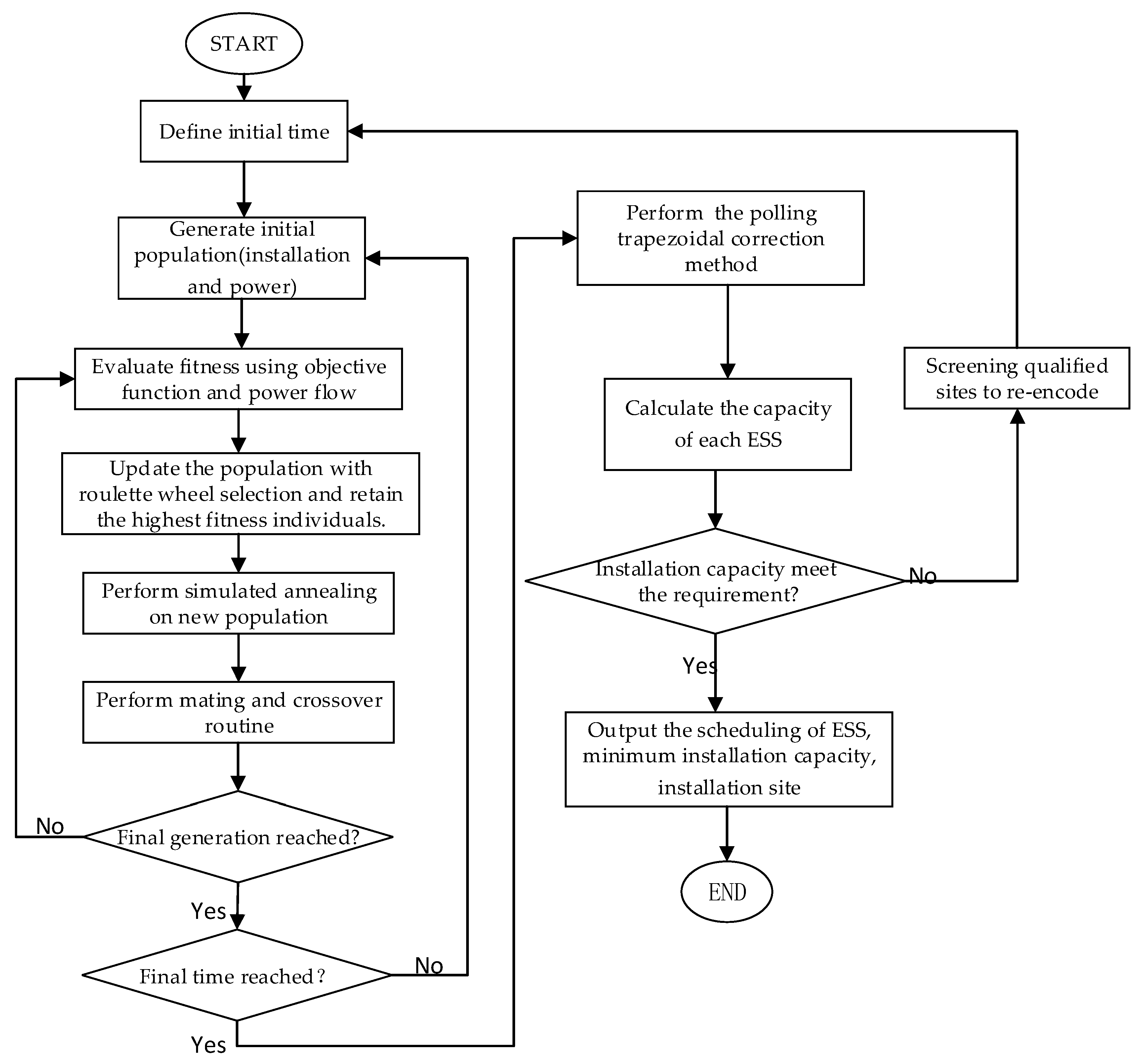
A two-stage planning strategy is proposed in this paper, and the schematic diagram of overall calculation process is illustrated in Figure 2. The first stage chooses the installation nodes and confirms the scheduling of ESS with the minimum installation capacity by utilizing GA combined with SA. The second stage optimizes the installation capacity of every installation nodes aiming at minimizing the LCC based on the output of the first stage.
3.1. The First-Stage Optimization
In this study, the overall optimization objective is to minimize the average annual cost of the ESS life cycle, on the premise that the ESS operates to stabilize voltage fluctuations. In the first stage, in order to effectively resolve the voltage fluctuations caused by the PV, the operation of ESSs are optimized with the objective of capital investment and line losses minimization, at time t. Then, the minimum installation capacity at the corresponding location is obtained. The installation sites are determined by the minimum installation capacity of the ESS at the pre-selected locations, including the critical load nodes, the end of the feeder, the DER busbars, and the primary substation, etc. The power output of individual storage at time t is considered as the rated power, and the capacity is calculated as the time over which the storage delivers full power, as in Equation (2), to meet the requirement of the ESS output at time t. The capital investment is the main concern at this stage, including the capital cost of the storage unit, the power conversion system (PCS), and the necessary supporting facilities. The cost of the storage unit and the cost of the necessary supporting facilities is proportional to the energy storage capacity and the cost of the power conversion equipment is proportional to the power rating of the system [17]. The cost of the ESS can be calculated as Equation (3).
where the capacity of ESS at node i is represented by Ei and D is the maximum depth of discharging. The µC/µD is the charging/discharging sign of the ESS, when the ESS is charging, µC is 1 and µD is 0, and when the ESS is discharging, µC is 0 and µD is 1. ηPCS is the nominal efficiency of the power conversion system and η is the round-trip efficiency. Δt is the duration of the charging/discharging. PESS,i(t) is the real charging/discharging power of node i at time t, and Cost1 is the capital investment of ESS, Cbat is the cost of the storage unit which can be calculated by Equation (4). CE is the price of ESS capacity per kW·h. The second term CPCS is the cost of the power conversion equipment which can be calculated by Equation (5), and CP is the charging cost per kW. The last term CBOP is the cost of the necessary supporting facilities which can be calculated by Equation (6), and CB is its cost per kW·h. Then Equation (3) can be rewritten as Equation (7).
The Optimization objective function of the GA combined with SA is presented as follows.
where Closs is the cost of line losses which can be calculated by the active power of the line loss multiplied by the average electricity price and Cpun is the cost of punishment applied by the utility for unsolved voltage issues.
The objective of the optimization is to minimize the ESS capital cost and line loss cost at this stage, so the fitness function of the GA can be represented by the reciprocal of the objective function as Equation (9).
Accumulating the charging/discharging energy of ESS through the output power PESS,i(t) from time 0 to time t which is obtained by GA, the energy fluctuation EESS,i(t) at time t of node i relative to the initial state of ESS at every installation nodes can be obtained [18].
For charging
For discharging
where EESS,i(t − 1) is the charging/discharging energy at time t − 1 of node i (EESS,i(0) = 0). ηC and ηD are the charging efficiency and discharging efficiency, respectively. The charging and discharging efficiencies are estimated as the root of the round-trip efficiency.
According to the energy fluctuations in the whole sampling cycle (which was one day, in this study), the difference between the maximum and minimum energy can be calculated. Then considering the limitations of the SOC, the minimization of capacity that must meet the ESS output can be obtained [15].
where E0,i is the minimum capacity that must meet the ESSs’ output. SOCmax and SOCmin are the minimum and maximum SOC limits of ESS. Ideally, the value of SOCmax is 1 and SOCmin is 0. To avoid the impact of over-charging/discharging during the battery lifetime, the short-cut process of SOCmax and SOCmin should be in the range of 0–1. max{EESS,i(t)} and min{EESS,i(t)}are the maximum and minimum energy fluctuation of the ESS in the whole sampling cycle, and max{EESS,i(t)} − min{EESS,i(t)} is the maximum range of the energy fluctuation.
The minimum installation capacity of the ESSs can be calculated by the charging and discharging power of each preferred node in the optimized period with Equations (10)–(12). In this study, if the minimum installation capacity E0,i of a preferred node was less than 10% of average capacity of each pre-selected nodes, the node was abandoned. The algorithm continued to optimize the capacity of the remaining preferred nodes, until the nodes and the capacities on the nodes met the requirement. Then the first-stage optimization was completed and the results were sent to the second stage.
3.2. The Second-Stage Optimization
3.2.1. Life-Cycle Cost Model
The expensive cost of the ESS is one of the biggest barriers impeding wide-area applications, at present, and this study proposed a comprehensive LCC model which considered various types of costs. The LCCs not only included the initial investment, but the operation and maintenance costs applied in the grid optimal planning, substation equipment maintenance, etc. [19]. Xue et al. considered the cost of the ESS with capital investment, replacement costs, operation and maintenance costs, and disposal cost [17]. Capital investment and replacement costs were the greatest proportion in the whole project cycle. Battery is one of the short-life equipment in the distribution system, frequent charging/discharging, and over charging/discharging can overwhelmingly reduce the lifetime and decrease the whole system economy. To reduce the replacement costs, expansion of the ESS capacity can be adopted, which can prolong the lifetime of the battery and reduce the replacement times. All of the costs considered in this study are presented as follows:
1. Capital investment
The main components of the ESS include the storage unit, the PCS, and the necessary supporting facilities, so the capital cost can be expressed as:
where Csys is the capital cost of battery. Erate and PESS,rate are the rated capacity and the power rating of the ESS, respectively, and the power rating is the maximum of the ESS charging/discharging power. Y is the project cycle (year) and σ is the discount rate (%). Apart from this, the other variables were same as shown in Equation (7).
The rated power can be evaluated as the minimum value of the maximum power allowed by the whole battery pack (Er∙Erate) and the maximum actual required charging/discharging power of ESS(PESS,max) [20]:
where Er is the energy rate of the ESS (kW/kW·h) and PESS,max is the maximum actual required charging/discharging power of the ESS. Generally, the maximum charging/discharging power of Li-ion batteries is strictly related to their rated capacity, so the typical parameter Er is used to represent the ratio between their maximum power and the rated capacity, the value of Er is set as 1 [20]. In some cases, the maximum power allowed by the battery could exceed the maximum actual required charging/discharging power, therefore, the minimum value should be chosen to guarantee economy of the ESS.
2. Replacement cost
The actual project cycle is generally 5 to 20 years. Although the lifetime of the supporting facilities can meet the project cycle need, the lifetime of the ESS and the PCS cannot be used for 20 years, without replacement. Annual replacement cost in the project cycle is formulated as Equation (15).
where β is the average annual decline rate of the ESS capital cost and k is the replacement times of battery (round up, k = Y/n − 1), n is the average lifetime of the chosen ESS, ε is the times of replacement. The lifetime of the PCS was chosen as 10 years, in this study [21].
3. Operation and maintenance cost
Operation and maintenance cost of ESS consists of fixed and variable operation and maintenance costs. The fixed operation and maintenance costs(CFOM) are composed of the labor cost and management cost, related to the types of ESS and the rated power. Then CFOM can be calculated as:
where Cf is the operation and maintenance cost per kW.
The variable operation and maintenance cost (CVOM) was changed with the status of real operation status and external variation, including electricity cost, fuel cost, renewable energy subsidies, and CO2 emission cost. In this study, only electricity cost was considered for simplicity. The annual average electricity cost (Cc), the duration of charging/discharging (Δt), and the number of operation days in a year (G) have an impact on the annual average electricity cost, which can be represented as:
4. Disposal cost
When the battery reaches the end of their life, the battery modules should be removed from the system and decommissioned, so the disposal costs of the ESS (Cdis) should be taken into account. The cost should be calculated when the battery needs to be replaced. According to Reference [11], there are mature methods for recovering and reusing some batteries like the lead–acid battery. However, the recovery of the Li-ion battery is still in its early stage. The main cost is due to the treatment of the materials constituting the ESS (hazardous and non-hazardous materials), so the disposal cost can be expressed as follows:
where Cd is a specific disposal cost per kW of the battery.
To sum up, the total cost of ESS in the whole project cycle is consisted of the capital costs, replacement costs, fixed/variable operation and maintenance cost, and disposal cost. It can be summarized as Cost 2:
The objective function aiming at minimizing the whole life-cycle cost of the ESS is expressed as
The fitness of the proposed GA should be the reciprocal of the objective function as in Equation (21).
3.2.2. Capacity Fading Model
At present, evaluating the lifetime of a battery is considered from the perspective of the degradation mechanisms, which cause the battery cell performance to deteriorate. When the degradation reaches a certain failure value, the end-of-life condition has been fulfilled. Conventionally, when the practical capacity of a battery has dropped to 80% of the battery’s original capacity, it reaches the end-of-life condition. So, the number of cycles (length of use) of the ESS, when the capacity is reduced to 80% of its initial capacity, is defined as cycle life (calendar life). There are many factors that cause capacity degradation, including dissolution of cathode materials, phase change of cathode materials, decomposition of electrolyte, overcharging, self-discharging, interfacial film formation, and fluid-collecting corrosion, etc. [22]. The capacity degradation is mainly manifested by a decreased in-solution concentration and an increased internal resistance of the battery, and it is related to the charging and discharging power, depth of discharging, fluctuation of SOC, number of cycles, and the operation temperature [22]. Lam, and Bauer, conducted a large number of tests and proposed a practical capacity fading model for Li-ion battery cells that can be especially used for irregular discharging, based on the experimental results [23]. The rest value of the Li-ion battery can be determined by the state-of-health (SOH) in this model. When the battery is at the initial capacity, the SOH is 1. If the SOH becomes 0, the battery reaches the end-of-life condition. The capacity fading rate is inseparable from the average SOC (SOCavg) and the SOC deviation (SOCdev), the higher the SOCavg or SOCdev, the higher the capacity fading rate [23]. The SOCavg represents the average SOC over the cycle τ (equal 24 h, in this study), and the SOCdev represents the normalized deviation of the SOC from its mean, over a cycle period. According to the SOC, temperature, depth of discharging, fluctuation of SOC, and charging/discharging power, SOCavg and SOCdev can be calculated and the total capacity fading is a summation of the capacity fading that occurs under the experienced operating conditions, and can be calculated as:
where Γ is the total capacity fade, according to Reference [23] the parameter Ks1 was set as −4.092 × 10⁻⁴, Ks2 was set as −2.167, Ks3 was chosen as −1.408 × 10⁻⁵, and Ks4 was set as 6.130. Parameters ks1 to ks4 were obtained through curve-fitting in the MATLAB Surface Fitting Tool, after analyzing the SoCdev influence on the measured capacity fading rates with both SoCavg and SoCdev as variables. Equation (22) was obtained by combining the fitting-curve and the Arrhenius equation, which can analyze the temperature-dependence of the capacity fading rate. Ea is the activation energy which was 78.06 kmol/J and R is the gas constant which was 8.314 J/(mol * K). An event is represented by I, which was a certain period τ, in this study, and is the total number of events. AhI represents the charging energy during event I. SOCavg,I and SOCdev,I are the average SOC and the SOC deviation, during event I. is the reference temperature in the operation process and is normally set to 25 °C. TI is the temperature of ESS in event I which can be formulated as Equation (23), according to the approximate linear relationship between the charging/discharging power and the temperature of Li-ion battery cells [24].
where Rth is the empirical constant and PESS(t) is the charging/discharging power of the ESS.
The SOC of the ESS in time t is determined by the SOC of ESS in time t − 1, charging/discharging energy, and power attenuation per hour, in the sampling period [t − 1, t] [3].
For charging, the SOC in time t can be calculated as:
For discharging, the SOC in time t can be calculated as:
where δ is the self-discharging rate of the ESS and SOC (t − 1) is the SOC in time t − 1.
The condition that the SOC always keeps in the constraints in the process of operation, must be considered, when calculating the initial value of SOC. According to Reference [15], the initial value of the SOC is described as:
The SOC changed from 1 to 0, when the total capacity fade reached 20% of the initial capacity, as in Equation (22). So, the SOH of the battery can be estimated as:
The lifetime of the battery n in Equation (15) was calculated, based on the time in Equation (22) (round, n = /365), where is the operation time of the Li-ion battery, in days.
4. Sitting and Sizing Optimization
The GA is an iterative heuristics optimization method which can better solve the nonlinear problem with constraints. However, the basic GA has the disadvantage of dropping into the local optimal solution, easily called a GA premature convergence [25]. SA is a general probability algorithm which allows a wide exploration of the searching space. It can apply some random changes to a population member, for a specific number of rounds. These changes are accepted if they improve the fitness of the solution. However, crucially, if these do not improve the fitness, they are accepted with a probability which decreases in every round [26]. Then the algorithm takes the current solution away from the local optimal solution. The global optimal solution can, thereby, be found. In order to solve the GA premature convergence issue, this study supplemented the GA with SA. For the proposed SA, the probability which decreases every round when the changes reduce the fitness can be calculated according to Equation (28) [27].
where, P is the accepted probability of a new population member that has a reduced fitness, after applying the annealing operation. Where, Fit is the fitness of the old population member, before the annealing operation, then the fitness of the new population member, after the annealing operation, is presented as Fitnew. α is the annealing coefficient and m is the number of annealing. T is the initial temperature of annealing.
The steps of GA combining with SA are presented as follows:
- Step 1: Randomly generate the initial population by binary encoding.
- Step 2: Calculate the objective function value of each population member.
- Step 3: Calculate and select the individuals with larger fitness from the population and constitute a new population.
- Step 4: Perform the annealing operations, according the probability represented in Equation (28).
- Step 5: On the basis of the population from step 3, get the new population by mating and the crossover routine.
- Step 6: Finally, if the final generation is reached or the convergence criteria is met, output the optimization results. Otherwise, return to step2.
This paper presents a two-stages ESS optimal planning approach, the first stage is to optimize the installation site, the optimization variables are the location and power output of each ESS, and Equation (9) is the optimization objective. The installation site, charging and discharging strategy, and the minimum installation capacity which can satisfy the scheduling of the ESSs, can be solved by using GA combined with SA. The specific process of the first stage is presented in Figure 3. In this stage, each of the four genes represents an energy-storage location, and the four gene bits encodes the ESS output power at this location, in binary. According to the results of the first-stage optimization, the second stage puts the rated capacity of each ESS as the optimization variables, which takes the minimum installation capacity E0,i of the first stage, as the lower limit of the capacity variable and Equation (21) as the optimization objective. Each ESS operates according to the prescribed charging and discharging strategy of the first stage, then the power rating can be confirmed by the Equation (14) and each SOC values, at all times, can be calculated using Equations (24)–(26). The lifetimes of the Li-ion batteries are determined through the practical capacity fading model, considering multiple types of costs. The rated capacity with the LCC minimization of each ESS is determined by utilizing the GA combined with the SA strategy. The specific process of this stage is presented as Figure 4. In this stage, each of the four genes represents an energy-storage location, and the four genes encodes the energy storage capacity at this location, in binary.
In order to maintain the energy balance of the ESS, the SOC at the end of a day must be equal to the initial SOC. So, the charging/discharging power of the ESS must be further optimized to ensure that the above condition can be satisfied. In this study, the polling trapezoidal correction method is adopted to correct the output of the ESS. The method sums up the ESS output energy for one day, and the result is assessed as ESUM. If ESUM > 0, then the discharging energy is greater than the charging energy of a day. So, the sampling point of which output is less than or equal to zero from top to bottom, in a time sequence, is searched for, then the sampling point with a fixed step-length is modified. After a sampling point is modified, whether the voltage constraint is fulfilled by the power-flow calculation is checked for. The modification is adopted when the constraint is met. If the value of the ESUM is still more than zero, then the next point is revised. If all sampling points in the cycle are corrected but the requirement is not met, the points should be revised in the same way from top to bottom, again, in the next cycle, until the requirement is satisfied. If ESUM < 0, that means the charging energy is greater than the discharging energy of a day. So, the sampling point of which output is more than or equal to zero, from the top to bottom, in the time sequence, is searched for, and then modified by the sampling point with a fixed step-length.
In addition, for the sake of improving the searching efficiency, the individuals with the highest fitness of each generation are directly put into the next generation population, to accelerate the convergence of the algorithm to retain the elite populations of the GA.
5. Case Studies
5.1. Profiles
In this section, the proposed method is implemented to the planning of the ESS, in a low-voltage distribution system, as shown in Figure 5. The parameters of the low-voltage case study distribution system are shown in the Table A1 of Appendix A. There were sixty-one nodes, in this case study network, and the base voltage was 10 kV, with the tight upper and lower limits of the voltage magnitude being 1.03 p.u. and 0.97 p.u., respectively. The node 451 was the slack bus and the node 150 was the standby node in the network. In this region, the time-of-use pricing mechanism was adopted. The electricity prices and time periods were: 0.976 ¥/(kW·h) from 08:00 to 21:00 (peak hours), 0.294 ¥/(kW·h) from 00:00 to 07:00, and 22:00 to 24:00 (off-peak hours). The sampling period was 1 h. The daily profiles of the loads and the output of PV are shown in Figure 6.
The Li-ion battery was selected as the ESS, in this study. The upper and lower limits of the SOC were 90% and 10%, respectively, and the overall round-trip efficiency of the ESS was set to 95%. The efficiency of the power conversion system ηPCS was 95% [21]. According to Reference [17], the project life cycle was 20 years, without considering the annual average decline rate of the battery-installation cost. For this study, the cost of unit energy was 3224 ¥/kW·h, the cost of unit power was 1085 ¥/kW, and the operation and maintenance cost was 155 ¥/kW·year. The specific disposal cost of the battery was 1582 ¥/kW [11] and the cost for the necessary supporting facilities was ignored, in this study, due to the use of the Li-ion battery, which did not require complicated supporting facilities. In addition, the discount rate was set as 10%.
5.2. Case Study Results
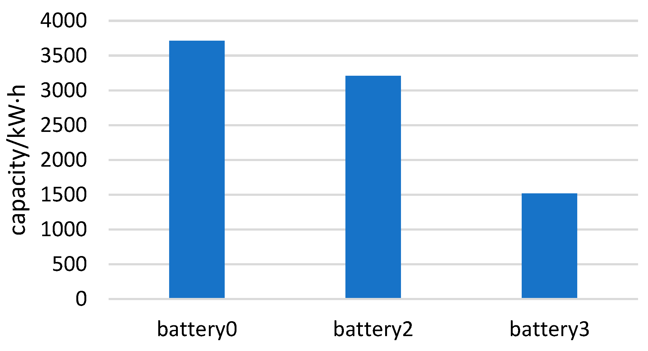
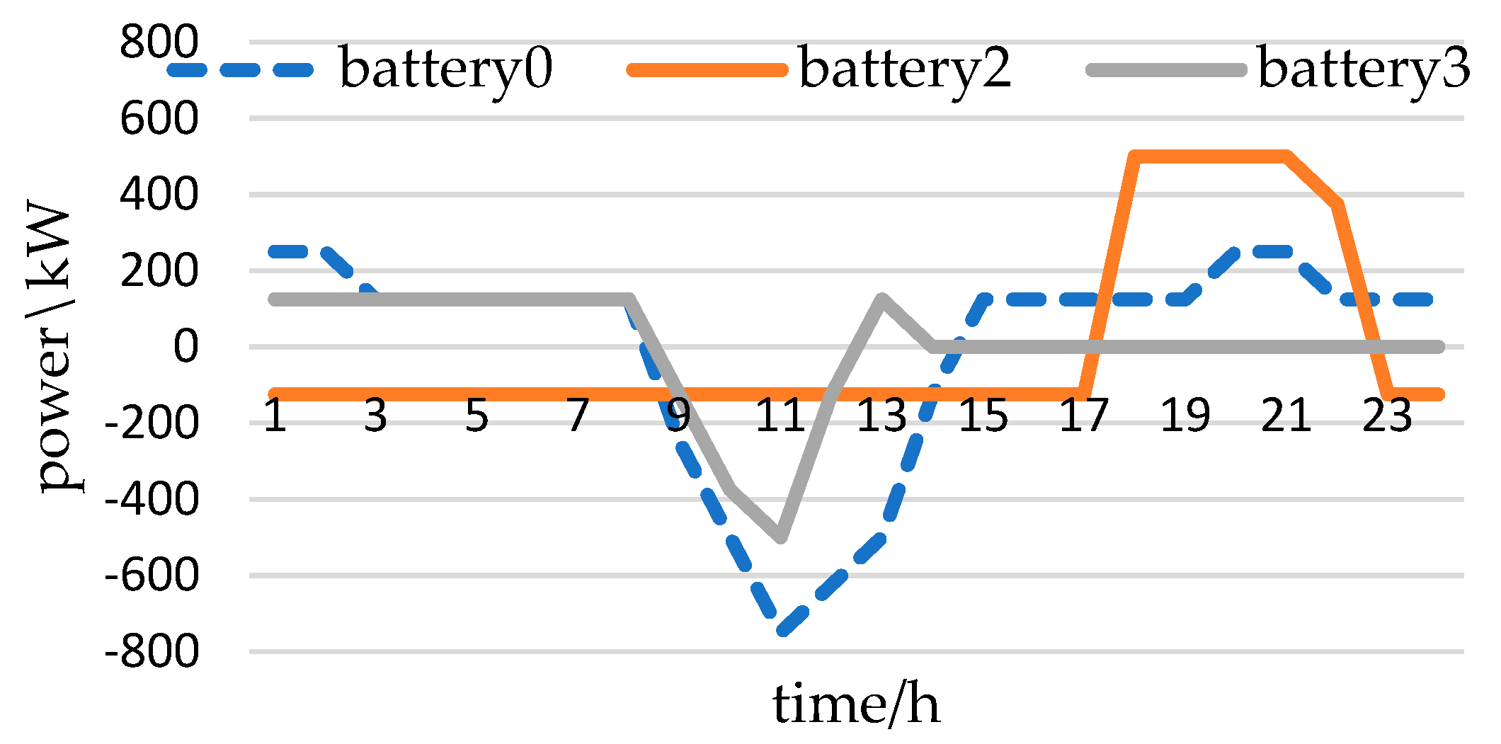
The ESS pre-selected candidate configuration nodes in the low-voltage distribution system are presented in Figure 5, and the parameters of the GA and the SA are shown in Table 1. ESS configuration locations and corresponding minimum configuration capacities, in the first-stage optimization, are shown in Figure 7. The output power of the ESS and voltage variation of each typical nodes are separately presented in Figure 8 and Figure 9. As shown in Figure 7, three installation nodes were selected from eight pre-selected nodes, and the installation capacity of node 3 was 3,712kW·h, the installation capacity of node 81 was 3,206kW·h, the installation capacity of node 84 was 1,519kW·h, after the first-stage optimization.
According to the results shown in Figure 8 and Figure 9, the scheduling of the ESS, after the first-stage optimization, could effectively solve the voltage issues with a minimum power output of the ESS. In this condition, when the PV output was large, during the day, the voltage magnitudes of some nodes which was close to the PV, exceed the upper limit. So, the ESS operated to absorb energy from the network to pull the voltage level back to the safety limit. When the loads increased during night, the voltage of some nodes that were close to demand would have exceeded the lower limit. So, the ESS operated to emit energy to the network, as sources to keep the voltage level in the safety limit. In addition, the output power of the adjacent battery 2, three were operated, coordinately, to stabilize voltage fluctuations caused by load 2 and PV2, with the consideration of the charging/discharging energy balance of a day. In order to improve the ESS utilization and the system economy, battery 2 and 3 could be combined as battery 2’ and battery 0 was presented as battery 0’, with same output as battery 0. The first-stage optimization was repeated to determine the optimal power and capacity, with the updated installation sites. As in Figure 10, the results showed that the optimized capacity after the merging of the adjacent batteries was obviously reduced and Figure 11 showed the output power of the ESS, after merging.
The second optimization stage was based on the result of the first stage, then the rated capacity and rated power of the ESS, of a day, could be determined by the method shown in Figure 4. The rated power and rated capacity is shown in Table 2. The lifetime and average annual cost of the ESS, before and after the second optimization stage are shown in Table 3, according to the results, although the optimization capacity of the ESS in the second stage was larger than the results calculated by the first stage, the lifetime expectancy was accompanied by capacity growth. The capacity of the ESS expansion extended its lifetime, so the average annual cost was substantially lower than the first stage. The average annual costs of battery 0’ and battery 2’ had dropped by 32.4% and 58.3%, separately, and the total average annual cost of the ESS had dropped by 47.3%. According to Reference [28], the total average annual cost of the ESS could be converted as per kW·h, by Equation (29).
where COE is the cost per kW·h of ESS.
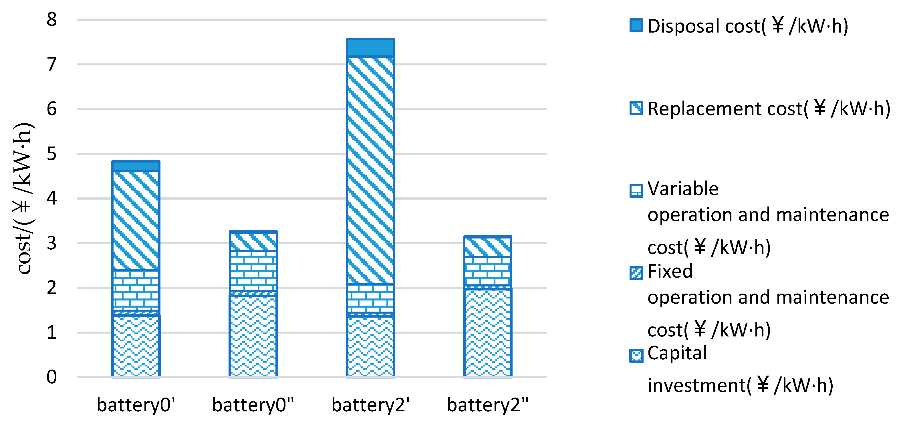
In Figure 12, battery 0” and battery 2” are used to represent the battery 0’ and battery 2’, after the second-stage optimization. The costs of the ESSs were effectively reduced after the second-stage optimization. The fixed and variable operation and maintenance costs which were related to the operating power, did not change after the second-stage optimization. Before the second-stage optimization, the replacement costs for battery 0’ and battery 2’ were 45.9% and 67.3% of the overall ESS cost, respectively, while the capital investments were 28.7% and 18%, respectively. After the second-stage optimization, the largest share of the overall ESS cost became the capital investment which were 55.6% and 62.5%, for battery 0” and battery 2”, respectively. The proportion of the replacement cost and the disposal cost were greatly reduced to 12.6% and 14% of the overall cost of battery 0” and battery 2”. Due to the decrease of the replacement times, the proportion of disposal costs of battery 0’ and battery 2’ changed from 4.5% to 0.9% and 5.1% to 0.7%, separately.
In the second-stage optimization, the discount rate, which was the interest rate, the converted values of the future assets into the present value was considered. The investment cost of the whole project cycle was counted, to the first year, by using the net present value (NPV), then the uniform annual value method was used to average it to each year of the project cycle. In this study, NPV was defined as the sum of the present values of the incoming and the outgoing cash flows, over a period of time, and the uniform annual value method was the present value of the annual cash flow, calculated on the average of the cash flow of the investment scheme, and the period (years) of its utility. In this way, the capacity expansion of the ESS led to the increase of capital costs but reduced the times of replacement. The replacement costs were also affected by the prolongation of lifetime, therefore, decreasing the cost of the first year of the project derived by the NPV. The overall replacement cost could be deducted significantly. The economic characteristic of the ESS is shown in Figure 13, as the capacity grew and lifetime extended, the economics of the ESS tended to improve. There were fluctuations that occurred along with the increase in capacity and life, the reason was that the lifetime of the battery had been prolonged with the capacity increases, but the times of battery replacement remained the same, during the project life cycle.
The results indicated that the proposed planning method in the distribution networks could optimize the ESS installation site and capacity, and improve the economic efficiency of the ESS by increasing the energy storage capacity, extending its service life, and reducing the annual cost in the condition of ensuring the safe operation of the system.
6. Conclusions
The randomness and variability of the DERs bring a stochastic nature to the distribution grid operation. In order to solve voltage fluctuations while decreasing the LCCs of the ESSs at the same time, a two-stage optimal sitting and sizing method was proposed for the distribution networks. The first stage optimized the installation site and the scheduling of the ESS, and the second stage made further economic optimization for capacity, by prolonging the ESSs’ lifetime. The proposed method could be applied in low-voltage distribution systems with a high penetration of the DERs, and the simulation results demonstrated the feasibility and effectiveness of the proposed planning method. The work of this study can be summarized as follows.
- (1)
- The intermittence of renewables integrated in the distribution grid led to the risk of voltage fluctuations, which could be effectively solved by a suitable ESS configuration in low-voltage distribution networks.
- (2)
- A two-stage optimization model was built to optimize the installation site and the capacity of the ESS, which consider the coupling effects between the sizing and sitting of the ESS and the optimal operation of the system, in the first stage, and consider the LCC of the ESS in the second stage. Through the two-stage optimization, the overall cost of the ESS in the project cycle could be effectively reduced. It is worth noting that the second-stage optimization reduces costs by extending the ESSs’ service life, the life-cycle cost is, therefore, reduced due to the significant deduction of the replacement and the disposal cost.
- (3)
- The two-stage solution method reduced the computation scale and the difficulty of optimization, with a higher computation efficiency.
- (4)
- The effectiveness of this method was verified by the case study. The results showed that the costs per kW·h of battery 0 and battery 2 had reduced by 32.4% and 58.3%, respectively, after the second-stage optimization. The voltage profiles were regulated within the pre-defined limits, the economy of the ESS was greatly improved through the optimization.
- (5)
- The optimization method used in this study was mainly verified for low-voltage AC distribution networks, and could be extended to the AC/DC hybrid distribution grids, in the near future.
- (6)
- The revenue in a competitive market environment, with various types of participants, could also be considered into the ESS planning, to maximize the benefits of the storage and the entire distribution grids.
Author Contributions
T.X., H.M. and W.W. conceived the idea of the study, conducted the research and wrote the most of the paper; H.Y.and Y.R. studied the characteristics of various types of ESSs; J.Z., H.Z. and Z.L. analyzed the case study network and contributed to finalizing this paper.
Funding
This research was funded by the China National Key Research & Development Program under grant numbers [2016YFB0900500 and 2016YFB0900503].
Conflicts of Interest
The authors declare no conflict of interest.
Nomenclature
| AhI | the charging energy during event I. | PS | the active power of main grid |
| Cost | the average annual cost of the ESS within project planning period | PL | the active power of load |
| Cost1 | the capital investment of ESS in the first-stage optimization | Ploss | the active power of line loss |
| Cost2 | the LCC of ESS in the second-stage optimization | Pijmin | the lower active power limits of line ij |
| Csys | the annual average capital cost of ESS | Pijmax | the upper active power limits of line ij |
| Cbat | the cost of storage unit | Pij | the actual active power on line ij |
| CE | the price of capacity per kW·h | PESS,i,rate | the rated power of ESS at node i |
| CPCS | the cost of the PCS | PESS,i | The output power of ESS at node i |
| CP | the charging cost at per kW of CPCS | PESS,i(t) | the real charging/discharging power of node i at time t |
| CBOP | the cost of the necessary supporting facilities | PESS,rate | the power rating of ESS |
| CB | the cost per kW·h of the necessary supporting facilities | R | the gas constant |
| Closs | the cost of line losses | Rth | the empirical constant |
| Cpun | the cost of punishment | SOCmax | the upper limits of the SOC |
| CFOP | the fixed operation and maintenance cost | SOCmin | the lower limits of the SOC |
| Cf | the operation and maintenance cost per kW | SOCi | the SOC value of node i |
| CVOM | the variable operation and maintenance cost | SOCavg,I | the average SOC during the event I |
| Cc | the electricity cost | SOCdev,I | the SOC deviation during the event I |
| Crep | the annual average replacement cost | SOC(t) | the SOC in time t |
| Cdis | the annual average disposal cost | T | the initial temperature of annealing |
| Cd | the specific disposal cost per kW of the battery | Tref | the reference temperature in the operation process |
| COE | the cost per kW·h of ESS. | TI | the temperature of ESS in event I |
| D | the maximum depth of discharging | Vmax | the upper voltage limits |
| Ei | the capacity of ESS at node i in the first-stage optimization | Vmin | the lower voltage limits |
| E0,i | the minimum capacity that must meet ESSs’ output | Vj | the actual voltage magnitude at node j |
| Erate | the rated capacity of ESS | Y | the project cycle (year) |
| EESS,i(t) | the energy fluctuation relative to the initial state of ESS at every installation nodes | β | the average annual decline rate of ESS capital cost |
| Er | the energy rate of the ESS (kW/kW·h) | η | the overall round-trip efficiency |
| Ea | the activation energy | ηD | the efficiencies of discharging |
| G | the number of operation days in a year | ηC | the efficiencies of charging |
| k | the times of battery replacement | ηPCS | the nominal efficiency of the PCS |
| m | the number of annealing | σ | the discount rate (%) |
| N | the number of nodes which must be configured with ESS | ε | the times of replacement |
| Nset | the number of nodes which are nodes for ESS pre-selection | Γ | the total fade capacity |
| n | the average lifetime of the chosen ESS | the total number of events | |
| P | the accepted probability of new population member | Δt | the duration of charging/discharging |
| PESS,sum | the total power output of ESSs in the distribution network | δ | the self-discharging rate of ESS |
| PESS,max | the maximum actual required charging/discharging power of ESS | µC | the charging sign of ESS |
| PDG | the active power of DG | µD | the discharging sign of ESS |
Appendix A

Table A1.
Line segment data from the case study.
| Node A | Node B | Length | Type | Node A | Node B | Length | Type |
|---|---|---|---|---|---|---|---|
| 1 | 2 | 0.33144 | LGJ150 | 78 | 80 | 0.42614 | LGJ150 |
| 1 | 3 | 0.47348 | LGJ150 | 80 | 81 | 0.42614 | LGJ150 |
| 1 | 7 | 0.56818 | LGJ240 | 81 | 82 | 0.42614 | LGJ150 |
| 3 | 4 | 0.37879 | LGJ150 | 82 | 83 | 0.42614 | LGJ150 |
| 3 | 5 | 0.61553 | LGJ150 | 81 | 84 | 0.42614 | LGJ150 |
| 5 | 6 | 0.47348 | LGJ150 | 84 | 85 | 0.42614 | LGJ150 |
| 7 | 8 | 0.37879 | LGJ240 | 97 | 98 | 0.52083 | LGJ240 |
| 8 | 12 | 0.42614 | LGJ150 | 98 | 99 | 0.104167 | LGJ240 |
| 8 | 9 | 0.42614 | LGJ150 | 99 | 100 | 0.056818 | LGJ240 |
| 8 | 13 | 0.56818 | LGJ240 | 100 | 450 | 0.151515 | LGJ240 |
| 202 | 14 | 0.80492 | LGJ150 | 149 | 1 | 0.75758 | LGJ240 |
| 13 | 34 | 0.28409 | LGJ150 | 160 | 67 | 0.66288 | LGJ240 |
| 13 | 152 | 0.000009 | LGJ150 | 152 | 52 | 0.75758 | LGJ240 |
| 14 | 11 | 0.47348 | LGJ150 | 52 | 53 | 0.37879 | LGJ240 |
| 14 | 10 | 0.47348 | LGJ150 | 53 | 54 | 0.23674 | LGJ240 |
| 15 | 16 | 0.71023 | LGJ150 | 54 | 55 | 0.52083 | LGJ240 |
| 15 | 17 | 0.66288 | LGJ150 | 54 | 57 | 0.66288 | LGJ240 |
| 34 | 15 | 0.18939 | LGJ150 | 55 | 56 | 0.52083 | LGJ240 |
| 67 | 68 | 0.37879 | LGJ150 | 57 | 58 | 0.47348 | LGJ240 |
| 67 | 72 | 0.52083 | LGJ150 | 57 | 60 | 0.142045 | LGJ240 |
| 67 | 97 | 0.47348 | LGJ240 | 58 | 59 | 0.47348 | LGJ240 |
| 68 | 69 | 0.52083 | LGJ150 | 60 | 160 | 0.000009 | LGJ150 |
| 69 | 70 | 0.61553 | LGJ150 | 60 | 61 | 0.104167 | LGJ240 |
| 70 | 71 | 0.52083 | LGJ150 | 60 | 620 | 0.47348 | LGJ240 |
| 72 | 73 | 0.52083 | LGJ150 | 620 | 62 | 0.000009 | LGJ150 |
| 72 | 76 | 0.37879 | LGJ150 | 62 | 63 | 0.33144 | LGJ240 |
| 73 | 74 | 0.66288 | LGJ150 | 63 | 64 | 0.66288 | LGJ240 |
| 74 | 75 | 0.75758 | LGJ150 | 64 | 65 | 0.80492 | LGJ240 |
| 76 | 77 | 0.75758 | LGJ150 | 65 | 66 | 0.61553 | LGJ240 |
| 77 | 78 | 0.18939 | LGJ150 | 9 | 202 | 0.000009 | LGJ150 |
| 78 | 79 | 0.42614 | LGJ150 | 150 | 201 | 0.000009 | LGJ150 |
References
- Manghani, R.; McCarthy, R. Global Energy Storage: 2017 Year Interview and 2018–2022 Outlook, GTM Research. 2018. Available online: https://www.woodmac.com/our-expertise/focus/Power--Renewables/Global-Energy-Storage/ (accessed on 27 August 2018).
- Amin, A.Z. Electricity Storage and Renewables: Costs and Markets To 2030, 3rd ed.; International Renewable Energy Agency: Abu Dhabi, Arab Emirates, 2017; pp. 1–131. ISBN 978-92-9260-038-9. [Google Scholar]
- Xiao, H.; Pei, W.; Yang, Y.H.; Qi, Z.P.; Kong, L. Energy storage capacity optimization for microgrid considering battery life and economic operation. High Volt. Eng. 2015, 41, 3256–3265. [Google Scholar] [CrossRef]
- Lin, S.B.; Han, M.X.; Zhao, G.P.; Niu, Z.H.; Hu, X.D. Capacity Allocation of Energy Storage in Distributed Photovoltaic Power System Based on Stochastic Prediction Error. Proc. CSEE 2013, 33, 25–33. [Google Scholar]
- Hu, G.Z.; Duan, S.X.; Cai, T.; Chen, C.S. Sizing and Cost Analysis of Photovoltaic Generation System Based on Vanadium Redox Battery. Trans. China Electrotech. Soc. 2012, 27, 260–267. [Google Scholar] [CrossRef]
- Tant, J.; Geth, F.; Six, D.; Tant, P.; Driesen, J. Multi-objective battery storage to improve PV integration in residential distribution grids. IEEE Trans. Sustain. Energy 2013, 4, 182–191. [Google Scholar] [CrossRef]
- Hung, D.Q.; Mithulananthan, N.; Bansal, R.C. Integration of PV and BES units in commercial distribution systems considering energy loss and voltage stability. Appl. Energy 2014, 11, 1162–1170. [Google Scholar] [CrossRef]
- Shi, N.; Luo, Y. Bi-Level Programming Approach for the Optimal Allocation of Energy Storage Systems in Distribution Networks. Appl. Sci. 2017, 7, 398. [Google Scholar] [CrossRef]
- Zhang, Y.X.; Ren, S.Y.; Dong, Z.Y.; Xu, Y.; Meng, K.; Zheng, Y. Optimal placement of battery energy storage in distribution networks considering conservation voltage reduction and stochastic load composition. IET Gener. Trans. Distrib. 2017, 11, 3862–3870. [Google Scholar] [CrossRef]
- Liu, H.A.; Li, D.Z.; Liu, Y.T.; Dong, M.Y.; Liu, X.N.; Zhang, H. Sizing Hybrid Energy Storage Systems for Distributed Power Systems under Multi-Time Scales. Appl. Sci. 2018, 8, 1453. [Google Scholar] [CrossRef]
- Marchi, B.; Pasetti, M.; Zanoni, S. Life cycle cost analysis for ESS optimal sizing. Energy Procedia 2017, 113, 127–134. [Google Scholar] [CrossRef]
- Bahramia, S.; Hadi Amini, M. A Decentralized Trading Algorithm for an Electricity Market with Generation Uncertainty. Appl. Energy 2018, 218, 520–532. [Google Scholar] [CrossRef]
- Sun, M.; Gui, X. Optimal allocation of energy storage system independent of time limits for specific load. Autom. Electr. Power Syst. 2018, 1–8. [Google Scholar] [CrossRef]
- Luo, X.; Wang, J.H.; Dooner, M.; Clarke, J. Overview of current development in electrical energy storage technologies and the application potential in power system operation. Appl. Energy 2015, 137, 511–536. [Google Scholar] [CrossRef]
- Wang, C.S.; Yu, B.; Xiao, J.; Guo, L. Sizing of Energy Storage Systems for Output Smoothing of Renewable Energy Systems. High Vol. Eng. 2015, 41, 3256–3265. [Google Scholar] [CrossRef]
- Demirocak, D.E.; Srinivasan, S.S.; Stefanakos, E.K. A Review on Nanocomposite Materials for Rechargeable Li-Ion Batteries. Appl. Sci. 2017, 7, 731. [Google Scholar] [CrossRef]
- Xue, J.H.; Ye, J.L.; Tao, Q.; Wang, D.S.; Sang, B.Y.; Yang, B. Economic Feasibility of User-Side Battery Energy Storage Based on Whole-Life-Cycle Cost Model. Power Syst. Technol. 2016, 40, 2471–2476. [Google Scholar] [CrossRef]
- Xiao, J.; Zhang, Z.Q.; Bai, L.Q.; Liang, H.S. Determination of the optimal installation site and capacity of battery energy storage system in distribution network integrated with distributed generation. IET Gener. Trans. Distrib. 2016, 10, 601–607. [Google Scholar] [CrossRef]
- Xiang, Y.P.; Wei, Z.N.; Sun, G.Q.; Sun, Y.H.; Shen, H.P. Life Cycle Cost Based Optimal Configuration of Battery Energy Storage System in Distribution Network. Power Syst. Technol. 2015, 39, 264–270. [Google Scholar]
- Marchi, B.; Zanoni, S.; Pasetti, M. A techno-economic analysis of Li-ion battery energy storage systems in support of PV distributed generation. In Proceedings of the 21st Summer School F. Turco of Industrial Systems Engineering, Naples, Italy, 13–15 September 2016. [Google Scholar]
- IRENA. Innovation Outlook-Renewable Mini-Grids. 2016. Available online: https://www.irena.org/publications/2016/Sep/Innovation-Outlook-Renewable-mini-grids (accessed on 10 November 2018).
- Li, F.B.; Xie, K.G.; Zhang, X.S.; Zhao, B.; Chen, J. Optimization of Coordinated Control Parameters for Hybrid Energy Storage System Based on Life Quantification. Autom. Electr. Power Syst. 2014, 38, 1–5. [Google Scholar] [CrossRef]
- Lam, L.; Bauer, P. Practial Capacity Fading Model for Li-Ion Battery Cells in Electric Vehicles. IEEE Trans. 2013, 28, 5910–5918. [Google Scholar] [CrossRef]
- Hoke, A.; Brissette, A.; Maksimovic, D.; Pratt, A.; Smith, K. Electric vehicle charge optimization including effects of lithium-ion battery optimization effects of lithium-ion battery degradation. In Proceedings of the 2011 IEEE Vehicle Power and Propulsion Conference, Chicago, IL, USA, 6–9 September 2011. [Google Scholar] [CrossRef]
- Wen, F.S.; Han, Z.X. Fault diagnosis of power system based on genetic algorithm and simulated annealing algorithm. Proc. CSEE 1994, 14, 29–35. [Google Scholar] [CrossRef]
- Crossland, A.F.; Jones, D.; Wade, N.S. Planning the location and rating of distributed energy storage in LV networks using a genetic algorithm with simulated annealing. Electr. Power Energy Syst. 2014, 59, 103–110. [Google Scholar] [CrossRef]
- Liu, K.Y.; Sheng, W.X.; Li, Y.H. Research on Reactive Power Optimization Based on Improved Genetic Simulated Annealing Algorithm. Power Syst. Technol. 2007, 31, 13–18. [Google Scholar] [CrossRef]
- Poonpun, P.; Jewell, W.T. Analysis of the Cost per Kilowatt Hour to Store Electricity. IEEE Trans. Energy Convers. 2008, 23, 529–534. [Google Scholar] [CrossRef]
Figure 1.
Characteristics of different batteries. (a) Technical characteristics; and (b) Economic and lifetime characteristics.
Figure 1.
Characteristics of different batteries. (a) Technical characteristics; and (b) Economic and lifetime characteristics.
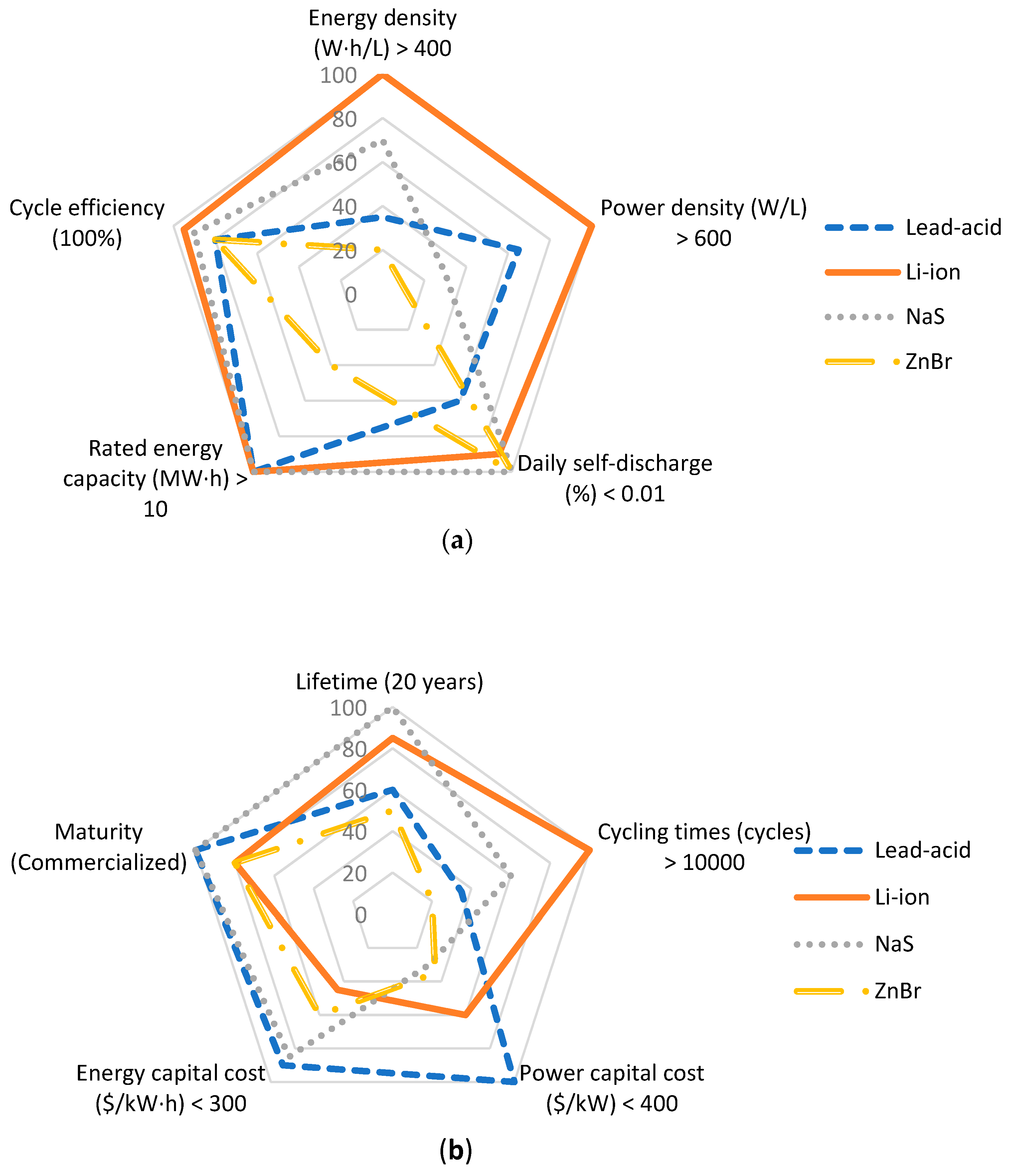
Figure 2.
Schematic diagram of the proposed two-stage optimal planning strategy.
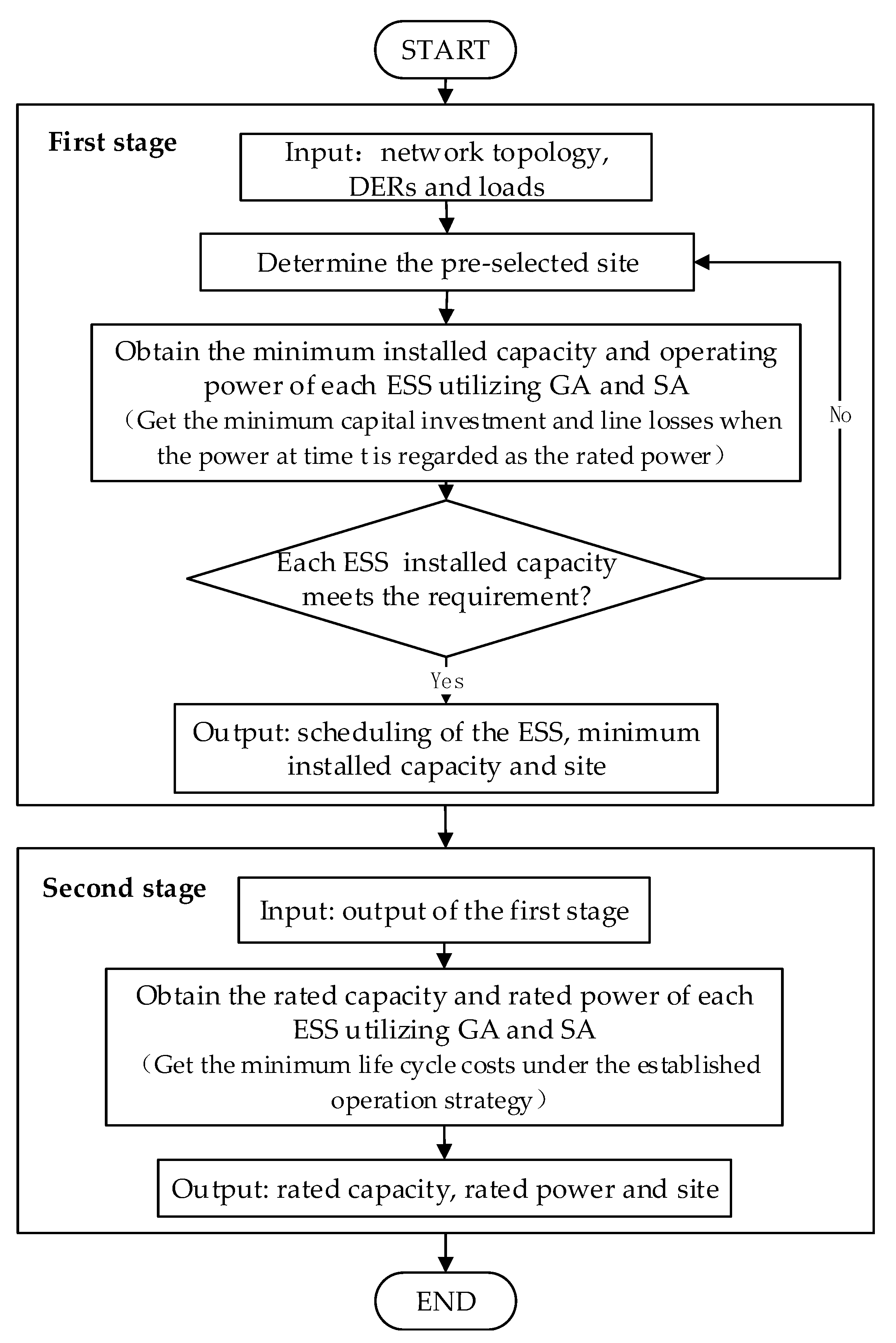
Figure 3.
Flowchart of the first-stage optimization.

Figure 4.
Flowchart of the second-stage optimization.
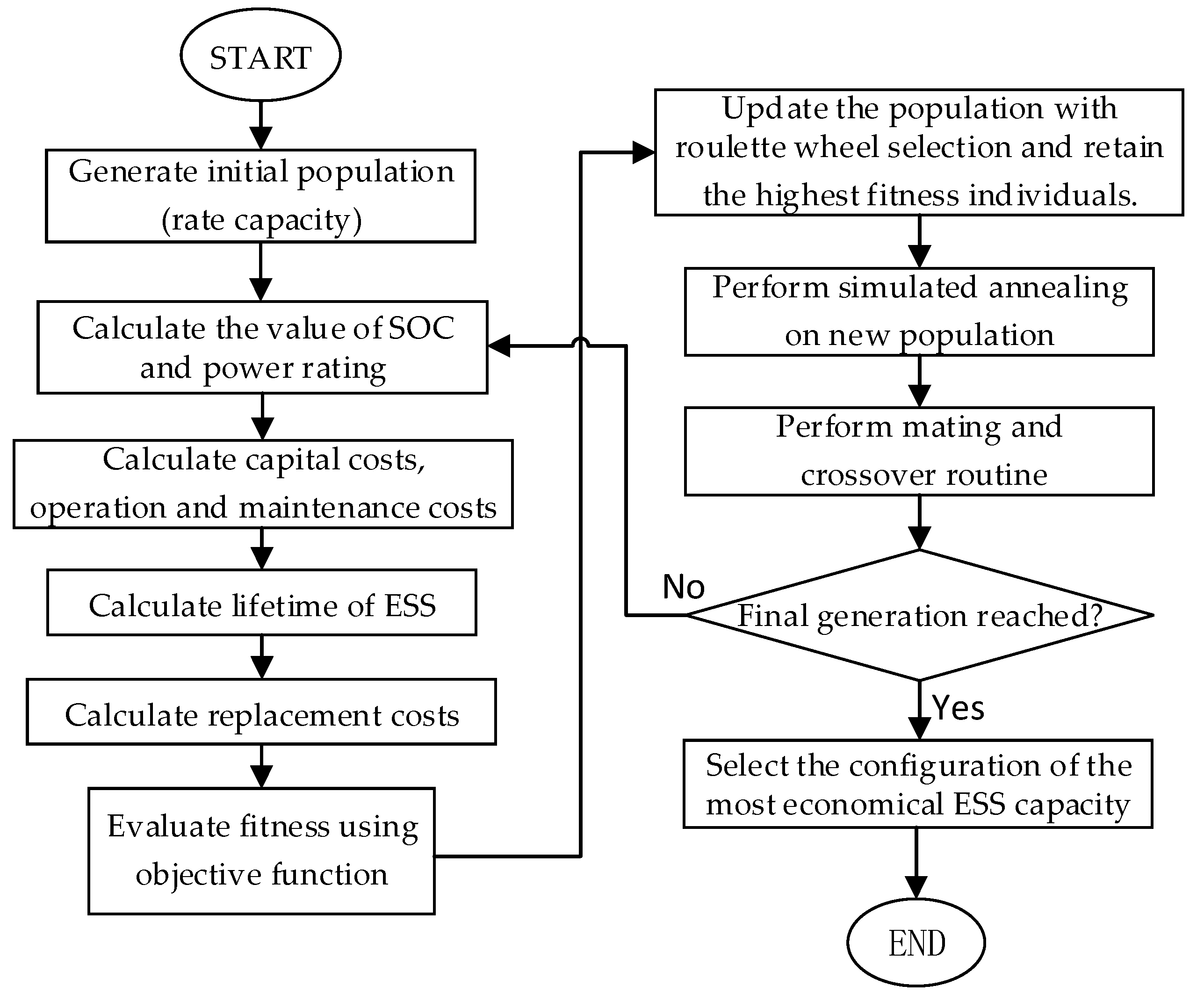
Figure 5.
A low-voltage case study distribution system.
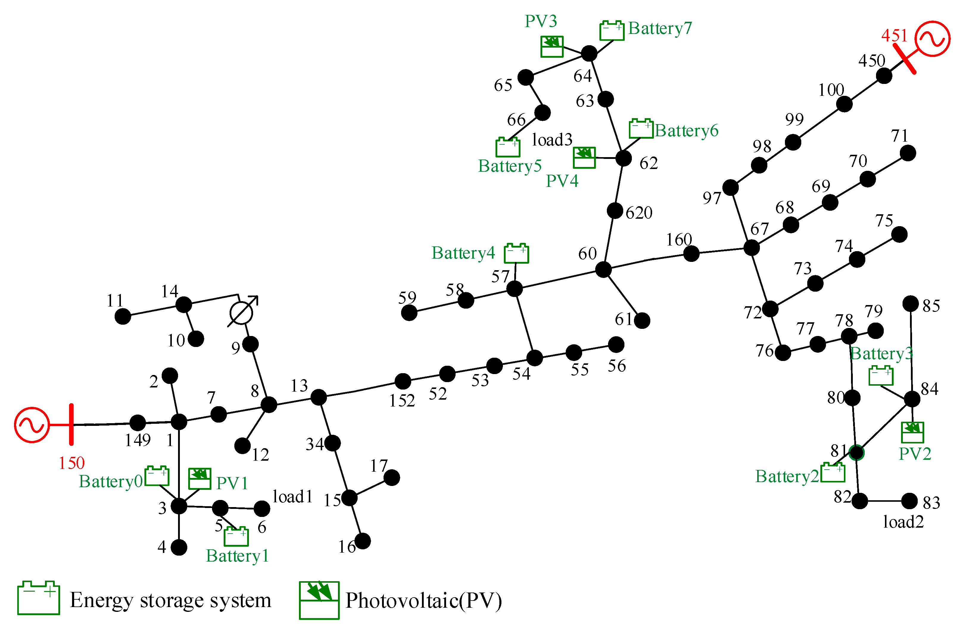
Figure 6.
Typical profiles of the loads and the Distributed Generation (DG) output.

Figure 7.
The Energy Storage System’s (ESS) sizing results after the first-stage optimization.

Figure 8.
Power output of the three planned ESSs.

Figure 9.
Voltage profiles of each typical node before (a) and after (b) the ESS configuration.
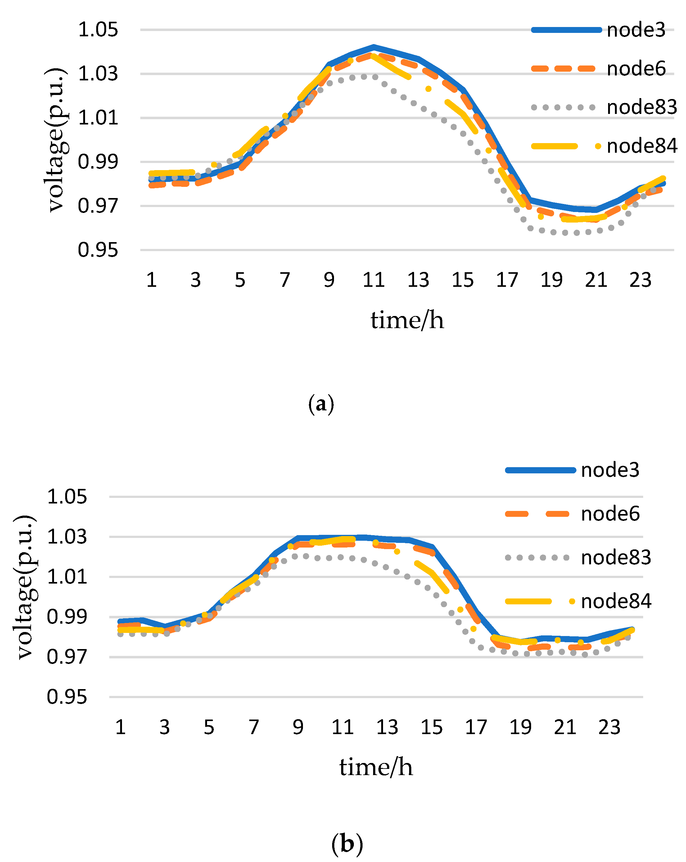
Figure 10.
Capacity comparison before and after the adjacent ESS merging.

Figure 11.
The power output of the ESSs after merging.
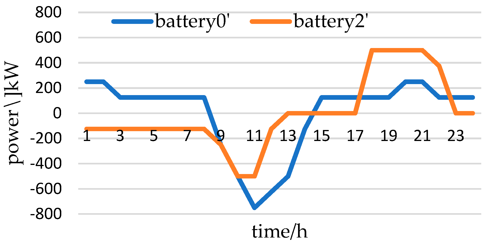
Figure 12.
Life-Cycle Cost (LCC) per kW·h comparison before and after the second-stage optimization.
Figure 12.
Life-Cycle Cost (LCC) per kW·h comparison before and after the second-stage optimization.

Figure 13.
The relationship of the capacity, lifetime, and average annual cost of the ESS.
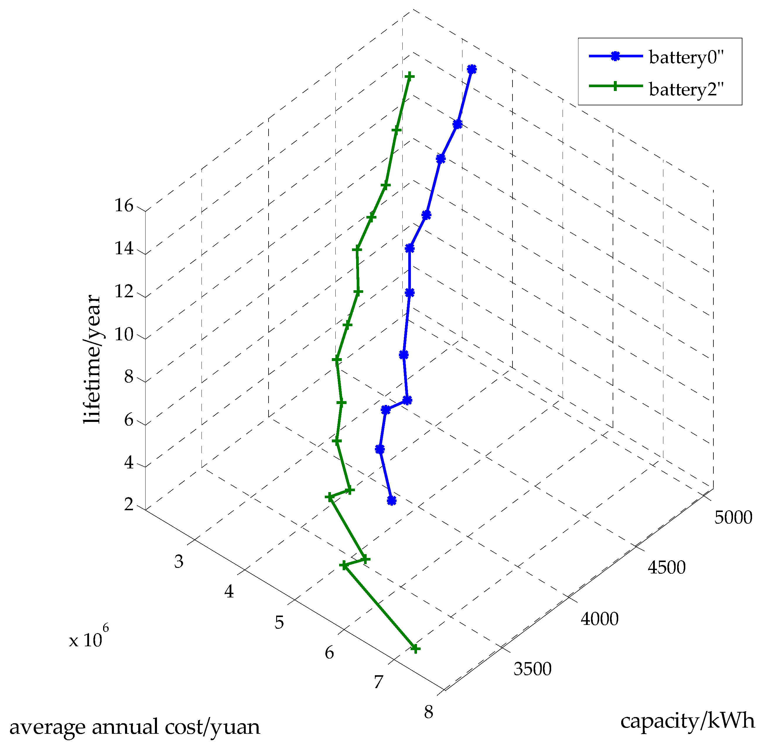
Table 1.
Parameters of the Genetic Algorithm (GA) and the Simulated Annealing (SA).
| Parameters of GA | Parameters of SA | ||||
|---|---|---|---|---|---|
| Maximum generation | 300 | Variation probability | 0.02 | Annealing coefficient | 0.95 |
| Size of population | 50 | Crossover rate | 0.7 | Initial temperature | 100 |
Table 2.
Configuration results of the second-stage optimization.
| Installation Site | Node 3 | Node 81 |
|---|---|---|
| Rated capacity(kW·h) | 4950 | 4703 |
| Rated power(kW) | 750 | 500 |
Table 3.
Lifetime and the average annual cost of the ESS.
| Optimization Stage | Installation Site | Lifetime/year | Average Annual Cost/¥ |
|---|---|---|---|
| First stage | Node 3 | 4 | 5,238,677 |
| Node 81 | 2 | 7,081,373 | |
| Second stage | Node 3 | 16 | 3,541,137 |
| Node 81 | 16 | 2,951,720 |
© 2018 by the authors. Licensee MDPI, Basel, Switzerland. This article is an open access article distributed under the terms and conditions of the Creative Commons Attribution (CC BY) license (http://creativecommons.org/licenses/by/4.0/).
Share and Cite
MDPI and ACS Style
Xu, T.; Meng, H.; Zhu, J.; Wei, W.; Zhao, H.; Yang, H.; Li, Z.; Ren, Y. Considering the Life-Cycle Cost of Distributed Energy-Storage Planning in Distribution Grids. Appl. Sci. 2018, 8, 2615. https://doi.org/10.3390/app8122615
AMA Style
Xu T, Meng H, Zhu J, Wei W, Zhao H, Yang H, Li Z, Ren Y. Considering the Life-Cycle Cost of Distributed Energy-Storage Planning in Distribution Grids. Applied Sciences. 2018; 8(12):2615. https://doi.org/10.3390/app8122615
Chicago/Turabian StyleXu, Tao, He Meng, Jie Zhu, Wei Wei, He Zhao, Han Yang, Zijin Li, and Yi Ren. 2018. "Considering the Life-Cycle Cost of Distributed Energy-Storage Planning in Distribution Grids" Applied Sciences 8, no. 12: 2615. https://doi.org/10.3390/app8122615
Note that from the first issue of 2016, this journal uses article numbers instead of page numbers. See further details here.