Characterization of the Light Field and Apparent Optical Properties in the Ocean Euphotic Layer Based on Hyperspectral Measurements of Irradiance Quartet

Abstract
:1. Introduction
2. Methods
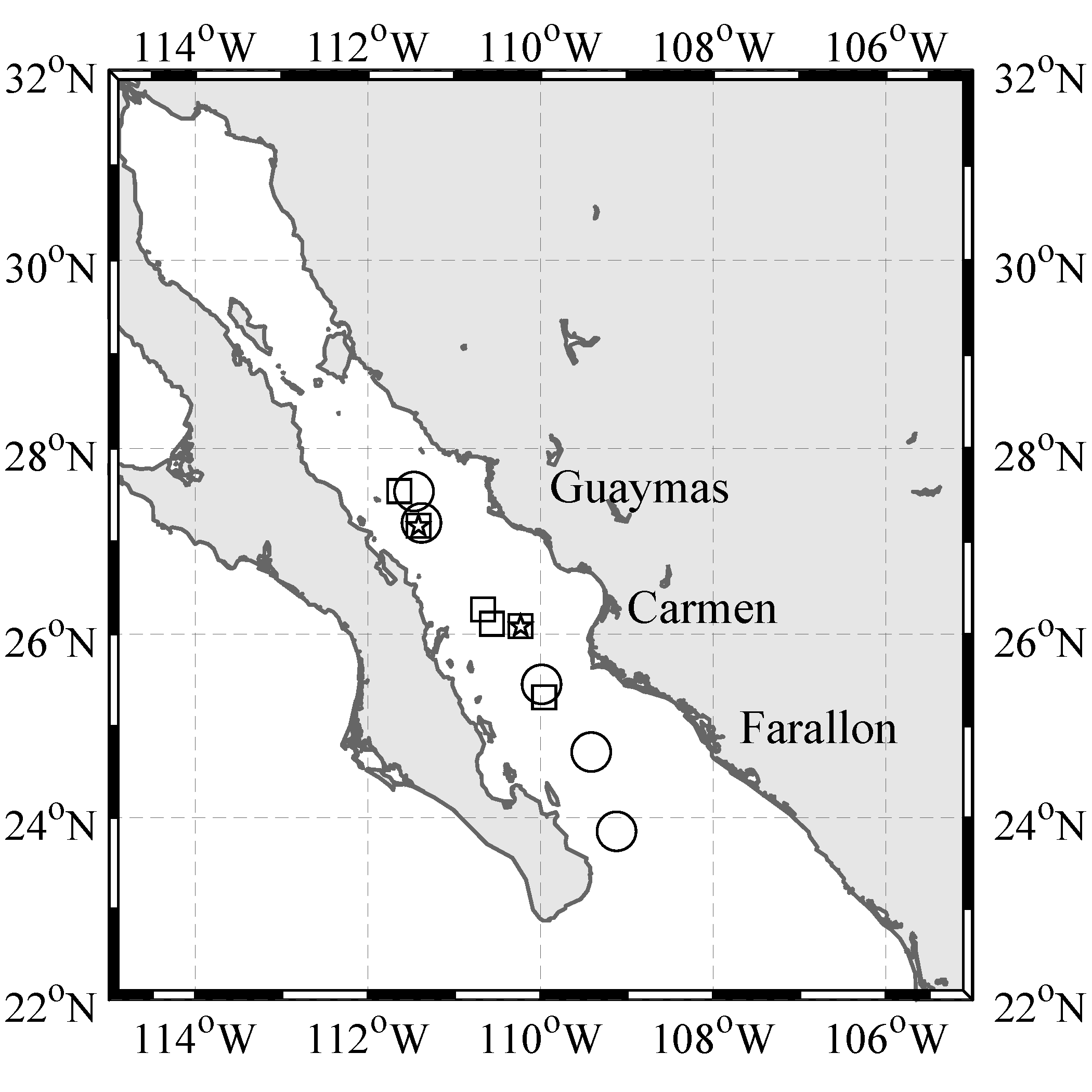
2.1. Study Area
2.2. CTD Measurements
2.3. Chlorophyll-a Concentration
2.4. Radiometric Quantities and Apparent Optical Properties
2.5. Absorption and Beam Attenuation Coefficients
2.6. Regression Analysis
3. Results and Discussion
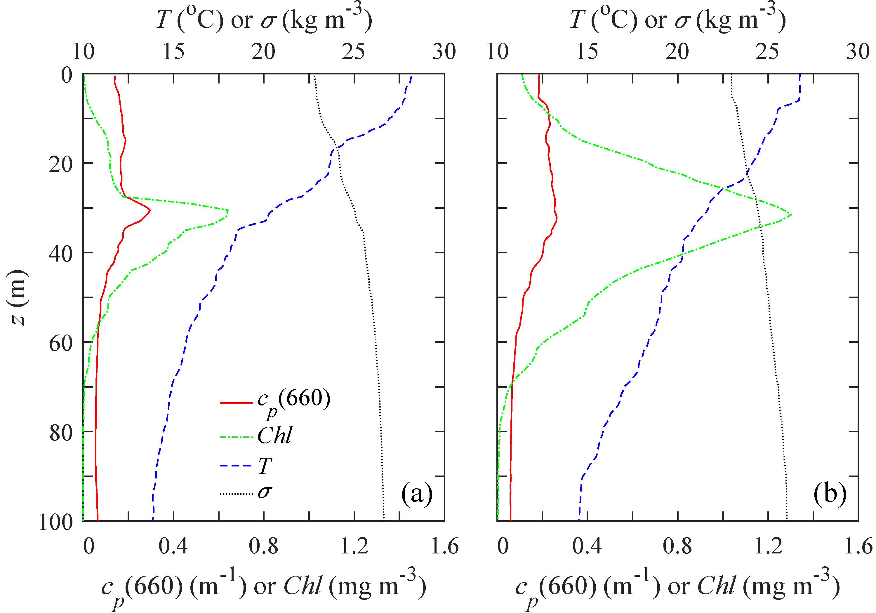
3.1. Contrasting Examples of Light Field Characteristics and AOPs
3.2. Overall Variability and Relationships Involving the Apparent Optical Properties
3.2.1. Average Cosines
3.2.2. Irradiance Reflectance
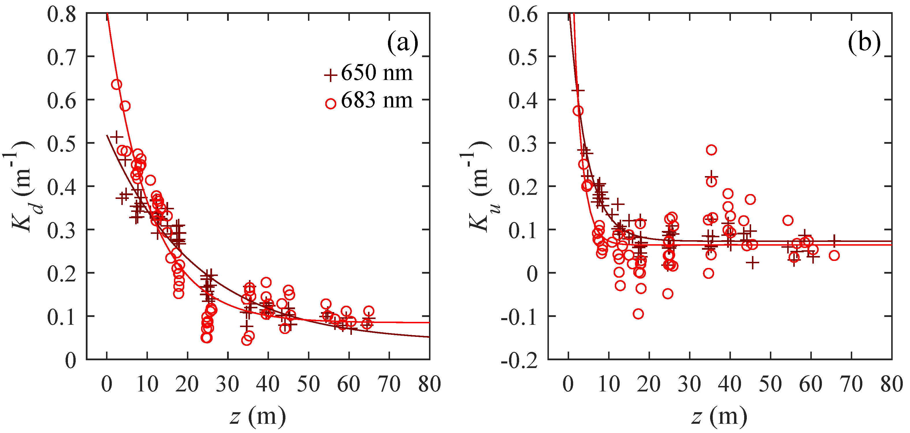
3.2.3. Diffuse Attenuation Coefficients
(r2 = 0.908, RMSE = 0.010 m−1, N = 54).
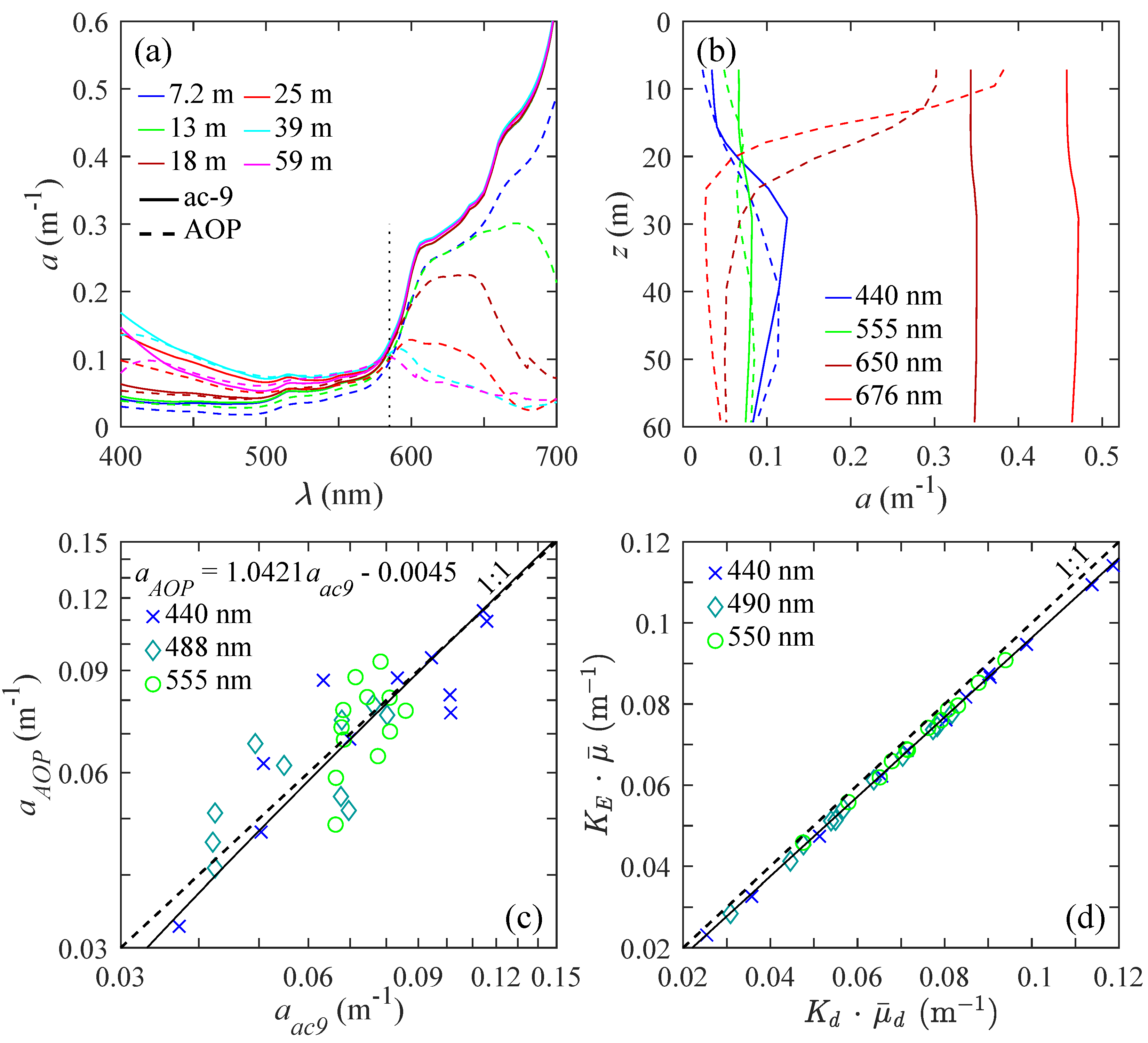
3.3. Application of Gershun’s Equation
4. Summary
Author Contributions
Acknowledgments
Conflicts of Interest
References
- Lewis, M.R.; Carr, M.E.; Feldman, G.C.; Esaias, W.; McClain, C. Influence of penetrating solar-radiation on the heat-budget of the equatorial Pacific Ocean. Nature 1990, 347, 543–545. [Google Scholar] [CrossRef]
- Lee, Z.P.; Du, K.P.; Arnone, R.; Liew, S.C.; Penta, B. Penetration of solar radiation in the upper ocean: A numerical model for oceanic and coastal waters. J. Geophys. Res. 2005, 110, C09019. [Google Scholar] [CrossRef]
- Field, C.B.; Behrenfeld, M.J.; Randerson, J.T.; Falkowski, P. Primary production of the biosphere: Integrating terrestrial and oceanic components. Science 1998, 281, 237–240. [Google Scholar] [CrossRef] [PubMed]
- Mobley, C.D.; Chai, F.; Xiu, P.; Sundman, L.K. Impact of improved light calculations on predicted phytoplankton growth and heating in an idealized upwelling-downwelling channel geometry. J. Geophys. Res. Oceans 2015, 120, 875–892. [Google Scholar] [CrossRef] [Green Version]
- Smith, R.C; Wilson, W.H., Jr. Photon scalar irradiance. Appl. Opt. 1972, 11, 934–938. [Google Scholar] [CrossRef] [PubMed]
- Booth, C.R. The design and evaluation of a measurement system for photosynthertically active quantum scalar irradiance. Limnol. Oceanogr. 1975, 21, 326–336. [Google Scholar] [CrossRef]
- Højerslev, N.K. Daylight measurements appropriate for photosynthetic studies in natural sea waters. J. Cons. Int. Explor. Mer 1978, 38, 131–146. [Google Scholar] [CrossRef]
- Morel, A. Available, usable, and stored radiant energy in relation to marine photosynthesis. Deep-Sea Res. 1978, 25, 673–688. [Google Scholar] [CrossRef]
- Mobley, C.D. Light and Water: Radiative Transfer in Natural Waters; Academic Press: San Diego, CA, USA, 1994. [Google Scholar]
- Kirk, J.T. Light and Photosynthesis in Aquatic Ecosystems; Cambridge University Press: Cambridge, UK, 1994. [Google Scholar]
- Jerlov, N.G. Marine Optics; Elsevier Scientific Publishing Company: Amsterdam, The Netherlands, 1976. [Google Scholar]
- Jerlov, N.G. Optical studies of ocean water. Rep. Swed. Deep-Sea Exped. 1951, 3, 1–59. [Google Scholar]
- Tyler, J.E.; Smith, R.C. Measurements of Spectral Irradiance Underwater; Gordon & Breach Publishing Group: Philadelphia, PA, USA, 1970. [Google Scholar]
- Jerlov, N.G.; Liljequist, G.H. On the angular distribution of submarine daylight and on the total submarine illumination. Svenska Hydrografisk-Biologiska Kommisionens Skrifter Ny Serie Hydrografi 1938, 14, 1–15. [Google Scholar]
- Whitney, L.V. The angular distribution of characteristic diffuse light in natural waters. J. Mar. Res. 1941, 4, 122–131. [Google Scholar]
- Smith, R.C. Structure of solar radiation in the upper layers of the sea. In Optical Aspects of Oceanography; Jerlov, N.G., Steemann, E., Eds.; Academic Press: San Diego, CA, USA, 1974; pp. 95–117. [Google Scholar]
- Lundgren, B.; Højerslev, N.K. Daylight Measurements in the Sargasso Sea: Results from the "Dana" Expedition January–April 1966. Report 14; University of Copenhagen, Institution of Physical Oceanography: Copenhagen, Denmark, 1971. [Google Scholar]
- Højerslev, N.K. Inherent and Apparent Optical Properties of the Western Mediterranean and the Hardangerfjord. Report 21; University of Copenhagen, Institution of Physical Oceanography: Copenhagen, Denmark, 1973. [Google Scholar]
- Ochakovskiy, Y.Y.; Kopelevich, O.V.; Voytov, V.I. Light in the Sea; (Edited translation from Russian) FTD-HT-24-105-72; Foreign Technology Division, Air Force System Command, US Air Force; National Technical Information Service, U.S. Department of Commerce: Springfieldm, VA, USA, 1972.
- Voss, K.J. Electro-optic camera system for measurement of the underwater radiance distribution. Opt. Eng. 1989, 28, 384–387. [Google Scholar] [CrossRef]
- Dickey, T.; Frye, D.; Jannasch, H.; Boyle, E.; Manov, D.; Sigurdson, D.; McNeil, J.; Stramska, M.; Michaels, A.; Nelson, N.; et al. Initial results from the Bermuda testbed mooring program. Deep Sea Res. Part I 1998, 45, 771–794. [Google Scholar] [CrossRef]
- Hooker, S.B.; Maritorena, S. An evaluation of oceanographic radiometers and deployment methodologies. J. Atmos. Ocean. Technol. 2000, 17, 811–830. [Google Scholar] [CrossRef]
- Clark, D.K.; Feinholz, M.; Yarbrough, M.; Johnson, B.C.; Brown, S.W.; Kim, Y.S.; Barnes, R.A. Overview of the radiometric calibration of MOBY. In Earth Observing Systems VI; Barres, W.L., Ed.; SPIE Proceedings; SPIE: Bellingham, WA, USA, 2002; Volume 4483, pp. 64–76. [Google Scholar] [CrossRef]
- Bulgarelli, B.; Zibordi, G.; Berthon, J.F. Measured and modeled radiometric quantities in coastal waters: Toward a closure. Appl. Opt. 2003, 42, 5365–5381. [Google Scholar] [CrossRef] [PubMed]
- Voss, K.J.; Chapin, A. Upwelling radiance distribution camera system, NURADS. Opt. Express 2005, 13, 4250–4262. [Google Scholar] [CrossRef] [PubMed]
- Morel, A.; Gentili, B.; Claustre, H.; Babin, M.; Bricaud, A.; Ras, J.; Tieche, F. Optical properties of the “clearest” natural waters. Limnol. Oceanogr. 2007, 52, 217–229. [Google Scholar] [CrossRef] [Green Version]
- Antoine, D.; d’Ortenzio, F.; Hooker, S.B.; Bécu, G.; Gentili, B.; Tailliez, D.; Scott, A.J. Assessment of uncertainty in the ocean reflectance determined by three satellite ocean color sensors (MERIS, SeaWiFS and MODIS-A) at an offshore site in the Mediterranean Sea (BOUSSOLE project). J. Geophys. Res. 2008, 113, C07013. [Google Scholar] [CrossRef]
- Chang, G.C.; Dickey, T.D. Interdisciplinary sampling strategies for detection and characterization of harmful algal blooms. In Real-Time Observation Systems for Ecosystem Dynamics and Harmful Algal Blooms; Babin, M., Roesler, C.S., Cullen, J.J., Eds.; UNESCO: Paris, France, 2008; pp. 43–84. [Google Scholar]
- Lewis, M.R.; Wei, J.; Van Dommelen, R.; Voss, K.J. Quantitative estimation of the underwater radiance distribution. J. Geophys. Res. 2011, 116, C00H06. [Google Scholar] [CrossRef]
- Wei, J.; Dommelen, R.V.; Lewis, M.R.; McLean, S.; Voss, K.J. A new instrument for measuring the high dynamic range radiance distribution in near surface sea water. Opt. Express 2012, 20, 27024–27038. [Google Scholar] [CrossRef] [PubMed]
- Antoine, D.; Morel, A.; Leymarie, E.; Houyou, A.; Gentili, B.; Victori, S.; Buis, J.-P.; Buis, N.; Meunier, S.; Canini, M.; et al. Underwater radiance distributions measured with miniaturized multispectral radiance cameras. J. Atmos. Ocean. Technol. 2013, 30, 74–95. [Google Scholar] [CrossRef]
- Cunningham, A.; McKee, D. Measurement of hyperspectral underwater light fields. In Subsea Optics and Imaging; Watson, J.E., Zielinski, O., Eds.; Woodhead Publishing: Philadelphia, PA, USA, 2013; pp. 83–97. [Google Scholar]
- Lewis, M.R. Measurement of apparent optical properties for diagonosis of harmful algal blooms. In Real-Time Observation Systems for Ecosystem Dynamics and Harmful Algal Blooms; Babin, M., Roesler, C.S., Cullen, J.J., Eds.; UNESCO: Paris, France, 2008; pp. 207–236. [Google Scholar]
- Zibordi, G.; Voss, K.J. In situ optical radiometry in the visible and near infrared. In Optical Radiometry for Ocean Climate Measurements; Zibordi, G., Donlon, C.J., Parr, A.C., Eds.; Academic Press: San Diego, CA, USA, 2014; pp. 248–305. [Google Scholar]
- Smith, R.C.; Baker, K.S. The bio-optical state of ocean waters and remote sensing. Limnol. Oceanogr. 1978, 23, 247–259. [Google Scholar] [CrossRef]
- Siegel, D.A.; Dickey, T.D. Observations of the vertical structure of the diffuse attenuation coefficient spectrum. Deep-Sea Res. 1987, 34, 547–563. [Google Scholar] [CrossRef]
- Dirks, R.W.J.; Spitzer, D. On the radiative transfer in the sea, including fluorescence and stratification effects. Limnol. Oceanogr. 1987, 32, 942–953. [Google Scholar] [CrossRef] [Green Version]
- Morel, A. Optical modeling of the upper ocean in relation to its biogenous matter content (case I waters). J. Geophys. Res. 1988, 93, 10749–10768. [Google Scholar] [CrossRef]
- Morel, A.; Maritorena, S. Bio-optical properties of oceanic waters: A reappraisal. J. Geophys. Res. 2001, 106, 7163–7180. [Google Scholar] [CrossRef] [Green Version]
- Zibordi, G.; D'Alimonte, D.; Berthon, J.-F. An evaluation of depth resolution requirements for optical profiling in coastal waters. J. Atmos. Ocean. Technol. 2004, 21, 1059–1073. [Google Scholar] [CrossRef]
- Yarbrough, M.A.; Houlihan, T.; Feinholz, M.; Flora, S.; Johnson, B.C.; Kim, Y.S.; Murphy, M.Y.; Ondrusek, M.; Clark, D. Results in coastal waters with high resolution in-situ spectral radiometry: The Marine Optical System ROV. In Coastal Ocean Remote Sensing; Frouin, R.J., Ed.; SPIE Proceedings; SPIE: Bellingham, WA, USA, 2007; Volume 6680, p. 66800I. [Google Scholar]
- Antoine, D.; Hooker, S.B.; Bélanger, S.; Matsuoka, A.; Babin, M. Apparent optical properties of the Canadian Beaufort Sea—Part 1: Observational overview and water column relationships. Biogeosciences 2013, 10, 4493–4509. [Google Scholar] [CrossRef]
- Lee, Z; Shaoling, S; Stavn, R.H. AOPs are not additive: On the biogeo-optical modeling of the diffuse attenuation coefficient. Front. Mar. Sci. 2018, 5, Article 8. [Google Scholar] [CrossRef]
- Pegau, W.S.; Cleveland, J.S.; Doss, W.; Kennedy, C.D.; Maffione, R.A.; Mueller, J.L.; Stone, R.; Trees, C.C.; Weidemann, A.D.; Wells, W.H.; et al. A comparison of methods for the measurement of the absorption coefficient in natural waters. J. Geophys. Res. 1995, 100, 13201–13220. [Google Scholar] [CrossRef]
- Preisendorfer, R.W. Application of radiative transfer theory to light measurements in the sea. Int. Union Geod. Geophys. Monogr. Symp. Radiant Energy Sea 1961, 10, 11–30. [Google Scholar]
- Preisendorfer, R.W. Hydrologic Optics. Volume I. Introduction; US Department of Commerce, National Oceanic and Atmospheric Administration, Environmental Research Laboratories: Honolulu, HI, USA, 1976.
- Kirk, J.T. Volume scattering function, average cosines, and the underwater light field. Limnol. Oceanogr. 1991, 36, 455–467. [Google Scholar] [CrossRef] [Green Version]
- Gordon, H.R. Modeling and simulating radiative transfer in the ocean. In Ocean Optics; Spinrad, R.W., Carder, K.L., Perry, M.J., Eds.; Oxford University Press: New York, NY, USA, 1994; pp. 3–39. [Google Scholar]
- Gershun, A. The light field. J. Math. Phys. 1939, 18, 51–151. [Google Scholar] [CrossRef]
- Tyler, J.E.; Richardson, W.H.; Holmes, R.W. Method for obtaining the optical properties of large bodies of water. J. Geophys. Res. 1959, 64, 667–673. [Google Scholar] [CrossRef]
- Højerslev, N.K. A spectral light absorption meter for measurements in the sea. Limnol. Oceanogr. 1975, 20, 1024–1034. [Google Scholar] [CrossRef] [Green Version]
- Spitzer, D.; Wernand, M.R. In situ measurements of absorption spectra in the sea. Deep-Sea Res. 1981, 28A, 165–174. [Google Scholar] [CrossRef]
- Gordon, H.R. Inverse methods in hydrologic optics. Oceanologia 2002, 44, 9–58. [Google Scholar]
- Gordon, H.R.; Brown, O.B.; Jacobs, M.M. Computed relationships between the inherent and apparent optical properties of a flat homogeneous ocean. Appl. Opt. 1975, 14, 417–427. [Google Scholar] [CrossRef] [PubMed]
- Kirk, J.T. Monte Carlo study of the nature of the underwater light field in, and of the relationship between optical properties of, turbid yellow waters. Aust. J. Mar. Freshw. Res. 1981, 32, 517–532. [Google Scholar] [CrossRef]
- Gordon, H.R. Absorption and scattering estimates from irradiance measurements: Monte Carlo simulations. Limnol. Oceanogr. 1991, 36, 769–777. [Google Scholar] [CrossRef] [Green Version]
- Sathyendranath, S.; Platt, T. Angular distribution of the submarine light field: Modification by multiple scattering. Proc. R. Soc. Lond. A 1991, 433, 287–297. [Google Scholar] [CrossRef]
- Stramska, M.; Stramski, D.; Mitchell, B.G.; Mobley, C.D. Estimation of the absorption and backscattering coefficients from in-water radiometric measurements. Limnol. Oceanogr. 2000, 45, 628–641. [Google Scholar] [CrossRef]
- Loisel, H.; Stramski, D. Estimation of inherent optical properties of natural waters from the irradiance attenuation coefficient and reflectance in the presence of Raman scattering. Appl. Opt. 2000, 39, 3001–3011. [Google Scholar] [CrossRef] [PubMed]
- Morel, A.; Gentili, B. Radiation transport within oceanic (case 1) water. J. Geophys. Res. 2004, 109, C06008. [Google Scholar] [CrossRef]
- Lewis, M.R.; Cullen, J.J.; Platt, T. Phytoplankton and thermal structure of the ocean: Consequences of nonuniformity in the chlorophyll profile. J. Geophys. Res. 1983, 88, 2565–2570. [Google Scholar] [CrossRef]
- Gordon, H.R. Diffuse reflectance of the ocean: Influence of nonuniform phytoplankton pigment profile. Appl. Opt. 1992, 31, 2116–2129. [Google Scholar] [CrossRef] [PubMed]
- Stramska, M.; Stramski, D. Effects of a nonuniform vertical profile of chlorophyll concentration on remote-sensing reflectance of the ocean. Appl. Opt. 2005, 44, 1735–1747. [Google Scholar] [CrossRef] [PubMed]
- Li, L.; Stramski, D.; Reynolds, R.A. Characterization of the solar light field within the ocean mesopelagic zone based on radiative transfer simulations. Deep Sea Res. Part I 2014, 87, 53–69. [Google Scholar] [CrossRef]
- Gordon, H. Remote sensing of optical properties in continuously stratified waters. Appl. Opt. 1978, 17, 1893–1897. [Google Scholar] [CrossRef] [PubMed]
- Yang, Q.; Stramski, D.; He, M.-X. Modeling the effects of near-surface plumes of suspended particulate matter on remote-sensing reflectance of coastal waters. Appl. Opt. 2013, 52, 359–374. [Google Scholar] [CrossRef] [PubMed]
- Stavn, R.H.; Weidemann, A.D. Optical modeling of clear ocean light fields: Raman scattering effects. Appl. Opt. 1988, 27, 4002–4011. [Google Scholar] [CrossRef] [PubMed]
- Marshall, B.R.; Smith, R.C. Raman scattering and in-water ocean optical properties. Appl. Opt. 1990, 29, 71–84. [Google Scholar] [CrossRef] [PubMed]
- Kattawar, G.W.; Xu, X. Filling in of Fraunhofer lines in the ocean by Raman scattering. Appl. Opt. 1992, 31, 6491–6500. [Google Scholar] [CrossRef] [PubMed]
- Ge, Y.; Gordon, H.R.; Voss, K.J. Simulation of inelastic-scattering contributions to the irradiance field in the ocean: Variation in Fraunhofer line depths. Appl. Opt. 1993, 32, 4028–4036. [Google Scholar] [CrossRef] [PubMed]
- Stavn, R.H. Effects of Raman scattering across the visible spectrum in clear ocean water: A Monte Carlo study. Appl. Opt. 1993, 32, 6853–6863. [Google Scholar] [CrossRef] [PubMed]
- Hu, C.; Voss, K.J. In situ measurements of Raman scattering in clear ocean water. Appl. Opt. 1997, 36, 6962–6967. [Google Scholar] [CrossRef] [PubMed]
- Berwald, J.; Stramski, D.; Mobley, C.D.; Kiefer, D.A. The effect of Raman scattering on the average cosine and the diffuse attenuation coefficient of irradiance in the ocean. Limnol. Oceanogr. 1998, 43, 564–576. [Google Scholar] [CrossRef]
- Gordon, H.R. Contribution of Raman scattering to water-leaving radiance: A reexamination. Appl. Opt. 1999, 38, 3166–3174. [Google Scholar] [CrossRef] [PubMed]
- Li, L.; Stramski, D.; Reynolds, R.A. Effects of inelastic radiative processes on the determination of water-leaving spectral radiance from extrapolation of underwater near-surface measurements. Appl. Opt. 2016, 55, 7050–7067. [Google Scholar] [CrossRef] [PubMed]
- Lavín, M.F.; Marinone, S.G. An overview of the physical oceanography of the Gulf of California. In Nonlinear Processes in Geophysical Fluid Dynamics; Velasco Fuentes, O.U., Sheinbaum, J., Ochoa, J., Eds.; Springer: Dordrecht, The Netherlands, 2003; pp. 173–204. [Google Scholar]
- Lluch-Cota, S.E.; Aragon-Noriega, E.A.; Arreguín-Sánchez, F.; Aurioles-Gamboa, D.; Bautista-Romero, J.J.; Brusca, R.C.; Cervantes-Duarte, R.; Cortés-Altamirano, R.; Del-Monte-Luna, P.; Esquivel-Herrera, A.; et al. The Gulf of California: Review of ecosystem status and sustainability challenges. Prog. Oceanogr. 2007, 73, 1–26. [Google Scholar] [CrossRef]
- Ras, J.; Claustre, H.; Uitz, J. Spatial variability of phytoplankton pigment distributions in the Subtropical South Pacific Ocean: Comparison between in situ and predicted data. Biogeosciences 2008, 5, 353–369. [Google Scholar] [CrossRef]
- Ritchie, R.J. Universal chlorophyll equations for estimating chlorophylls a, b, c, and d and total chlorophylls in natural assemblages of photosynthetic organisms using acetone, methanol, or ethanol solvents. Photosynthetica 2008, 46, 115–126. [Google Scholar] [CrossRef]
- Gordon, H.R. Ship perturbation of irradiance measurements at sea 1: Monte Carlo simulations. Appl. Opt. 1985, 24, 4172–4182. [Google Scholar] [CrossRef] [PubMed]
- Waters, K.J.; Smith, R.C.; Lewis, M.R. Avoiding ship-induced light-field perturbation in the determination of oceanic optical properties. Oceanography 1990, 3, 18–21. [Google Scholar] [CrossRef]
- Zibordi, G.; Darecki, M. Immersion factors for the RAMSES series of hyper-spectral underwater radiometers. J. Opt. A Pure Appl. Opt. 2006, 8, 252–258. [Google Scholar] [CrossRef]
- Stramski, D. Fluctuations of solar irradiance induced by surface waves in the Baltic. Bull. Pol. Acad. Sci. Earth Sci. 1986, 34, 333–344. [Google Scholar]
- Darecki, M.; Stramski, D.; Sokólski, M. Measurements of high-frequency light fluctuations induced by sea surface waves with an Underwater Porcupine Radiometer System. J. Geophys. Res. 2011, 116, C00H09. [Google Scholar] [CrossRef]
- Sullivan, J.M.; Twardowski, M.S.; Zaneveld, J.R.V.; Moore, C.M.; Barnard, A.H.; Donaghay, P.L.; Rhoades, B. Hyperspectral temperature and salt dependencies of absorption by water and heavy water in the 400-750 nm spectral range. Appl. Opt. 2006, 45, 5294–5309. [Google Scholar] [CrossRef] [PubMed]
- Sokal, R.R.; Rohlf, F.J. Biometry: The Principles and Practice of Statistics in Biological Research, 3rd ed.; W.H. Freeman: New York, NY, USA, 1995. [Google Scholar]
- Banse, K. Should we continue to use the 1% light depth convention for estimating the compensation depth of phytoplankton for another 70 years. Limnol. Oceanogr. Bull. 2004, 13, 49–52. [Google Scholar] [CrossRef]
- Sugihara, S.; Kishino, M.; Okami, N. Contribution of Raman scattering to upward irradiance in the sea. J. Oceanogr. Soc. Jpn. 1984, 40, 397–404. [Google Scholar] [CrossRef]
- Bristow, M.; Nielsen, D.; Bundy, D.; Furtek, R. Use of water Raman emission to correct airborne laser fluorosensor data for effects of water optical attenuation. Appl. Opt. 1981, 20, 2889–2906. [Google Scholar] [CrossRef] [PubMed]
- Hoge, F.E.; Swift, R.N. Airborne simultaneous spectroscopic detection of laser-induced water Raman backscatter and fluorescence from chlorophyll a and other naturally occurring pigments. Appl. Opt. 1981, 20, 3197–3205. [Google Scholar] [CrossRef] [PubMed]
- Stramski, D.; Tęgowski, J. Effects of intermittent entrainment of air bubbles by breaking wind waves on ocean reflectance and underwater light field. J. Geophys. Res. 2001, 106, 31345–31360. [Google Scholar] [CrossRef] [Green Version]
- Bannister, T.T. Model of the mean cosine of underwater radiance and estimation of underwater scalar irradiance. Limnol. Oceanogr. 1992, 37, 773–780. [Google Scholar] [CrossRef] [Green Version]
- Berwald, J.; Stramski, D.; Mobley, C.D.; Kiefer, D.A. Influences of absorption and scattering on vertical changes in the average cosine of the underwater light field. Limnol. Oceanogr. 1995, 40, 1347–1357. [Google Scholar] [CrossRef] [Green Version]
- Aas, E.; Højerslev, N.K. Analysis of underwater radiance observations: Apparent optical properties and analytic functions describing the angular radiance distribution. J. Geophys. Res. 1999, 104, 8015–8024. [Google Scholar] [CrossRef] [Green Version]
- Sathyendranath, S.; Platt, T. Ocean-color model incorporating transspectral processes. Appl. Opt. 1998, 37, 2216–2227. [Google Scholar] [CrossRef] [PubMed]
- Nahorniak, J.S.; Abbott, M.R.; Letelier, R.M.; Pegau, W.S. Analysis of a method to estimate chlorophyll-a concentration from irradiance measurements at varying depths. J. Atmos. Ocean. Technol. 2001, 18, 2063–2073. [Google Scholar] [CrossRef]
- Brown, C.A.; Huot, Y.; Purcell, M.J.; Cullen, J.J.; Lewis, M.R. Mapping coastal optical and biogeochemical variability using an autonomous underwater vehicle and a new bio-optical inversion algorithm. Limnol. Oceanogr. Methods 2004, 2, 262–281. [Google Scholar] [CrossRef]
- Xing, X.; Morel, A.; Claustre, H.; d’Ortenzio, F.; Poteau, A. Combined processing and mutual interpretation of radiometry and fluorometry from autonomous profiling Bio-Argo floats: 2. Colored dissolved organic matter absorption retrieval. J. Geophys. Res. 2012, 117, C04022. [Google Scholar] [CrossRef]
- Westberry, T.K.; Boss, E.; Lee, Z. Influence of Raman scattering on ocean color inversion models. Appl. Opt. 2013, 52, 5552–5561. [Google Scholar] [CrossRef] [PubMed]
- Liu, C.C.; Carder, K.L.; Miller, R.L.; Ivey, J.E. Fast and accurate model of underwater scalar irradiance. Appl. Opt. 2002, 41, 4962–4974. [Google Scholar] [CrossRef] [PubMed]
- Liu, C.C.; Miller, R.L.; Carder, K.L.; Lee, Z.; D’Sa, E.J.; Ivey, J.E. Estimating the underwater light field from remote sensing of ocean color. J. Oceanogr. 2006, 62, 235–248. [Google Scholar] [CrossRef] [Green Version]
- Sathyendranath, S.; Platt, T. Computation of aquatic primary production: Extended formalism to include effect of angular and spectral distribution of light. Limnol. Oceanogr. 1989, 34, 188–198. [Google Scholar] [CrossRef] [Green Version]
- O’Reilly, J.E.; Maritorena, S.; Mitchell, B.G.; Siegel, D.A.; Carder, K.L.; Garver, S.A.; Kahru, M.; McClain, C. Ocean color chlorophyll algorithms for SeaWiFS. J. Geophys. Res. 1998, 103, 24937–24953. [Google Scholar] [CrossRef] [Green Version]
- O’Reilly, J.E.; Maritorena, S.; Siegel, D.A.; O’Brien, M.C.; Hooker, S.B.; Smith, R.; Menzies, D.; Mueller, J.L.; Kahru, M.; Toole, D.; et al. SeaWiFS Postlaunch Calibration and Validation Analyses, Part. 3, NASA/TM-2000-206892; Hooker, S.B., Firestone, E.R., Eds.; NASA Goddard Space Flight Center: Greenbelt, MD, USA, 2000; Volume 11.
- Smith, R.C.; Baker, K.S. Optical classification of natural waters. Limnol. Oceanogr. 1978, 23, 260–267. [Google Scholar] [CrossRef]
- Gordon, H.R.; Morel, A. Remote Assessment of Ocean Color for Interpretation of Satellite Visible Imagery: A Review; Springer: New York, NY, USA, 1983. [Google Scholar]
- Smith, R.C.; Baker, K.S. Optical properties of the clearest natural waters (200–800 nm). Appl. Opt. 1981, 20, 177–184. [Google Scholar] [CrossRef] [PubMed]
- Frouin, R.; Lingner, D.W.; Gautier, C.; Baker, K.S.; Smith, R.C. A simple analytical formula to compute clear sky total and photosynthetically available solar irradiance at the ocean surface. J. Geophys. Res. 1989, 94, 9731–9742. [Google Scholar] [CrossRef]
- Morel, A. Optical properties and radiant energy in the waters of the Guinea dome and the Mauritanian upwelling area in relation to primary production. J. Cons. Int. Explor. Mer 1982, 180, 94–107. [Google Scholar]
- Siegel, D.A.; Dickey, T.D. On the parameterization of irradiance for open ocean photoprocesses. J. Geophys. Res. 1987, 92, 14648–14662. [Google Scholar] [CrossRef]
- Smith, R.C.; Marra, J.; Perry, M.J.; Baker, K.S.; Swift, E.; Buskey, E.; Kiefer, D.A. Estimation of a photon budget for the upper ocean in the Sargasso Sea. Limnol. Oceanogr. 1989, 34, 1673–1693. [Google Scholar] [CrossRef] [Green Version]
- Moore, C.C.; Bruce, E.J.; Pegau, W.S.; Weidemann, A.D. WET Labs ac-9: Field calibration protocol, deployment techniques, data processing, and design improvements. In Ocean Optics XIII; SPIE Proceedings; SPIE: Bellingham, WA, USA, 1997; Volume 2963, pp. 725–731. [Google Scholar] [CrossRef]
- Twardowski, M.S.; Sullivan, J.M.; Donaghay, P.L.; Zaneveld, J.R.V. Microscale quantification of the absorption by dissolved and particulate material in coastal waters with an ac-9. J. Atmos. Ocean. Technol. 1999, 16, 691–707. [Google Scholar] [CrossRef]
- Röttgers, R.; McKee, D.; Woźniak, S.B. Evaluation of scatter corrections for ac-9 absorption measurements in coastal waters. Methods Oceanogr. 2013, 7, 21–39. [Google Scholar] [CrossRef]
- Sathyendranath, S.; Platt, T. The spectral irradiance field at the surface and in the interior of the ocean: A model for applications in oceanography and remote sensing. J. Geophys. Res. 1988, 93, 9270–9280. [Google Scholar] [CrossRef]


| Symbol | Description | Units |
|---|---|---|
| λ | Light wavelength in vacuum | nm |
| z | Depth in water | m |
| θs | Solar zenith angle | degree |
| a | Absorption coefficient | m−1 |
| b | Scattering coefficient | m−1 |
| c | Beam attenuation coefficient (sum of a and b) | m−1 |
| Lu | Spectral upwelling radiance at zenith direction | W m−2 sr−1 nm−1 |
| Ed, Eu | Spectral downwelling and upwelling plane irradiances | W m−2 nm−1 |
| Eo, Eod, Eou | Spectral total, downwelling, and upwelling scalar irradiances | W m−2 nm−1 |
| Kx | Diffuse attenuation coefficients for irradiance or radiance x | m−1 |
| , , | Average cosines of total, down- and upwelling light fields | dimensionless |
| R | Irradiance reflectance | dimensionless |
| Chl | Chlorophyll-a concentration | mg m−3 |
| Subscripts | ||
| w | Water | |
| p | Suspended particulate matter | |
| g | Colored dissolved organic matter (CDOM) |
| Depth of Measurement | Shallowest | Greatest | Chl Maximum |
|---|---|---|---|
| z (m) | 5.4 ± 2.9 | 64.9 ± 12.1 | 33.0 ± 9.9 |
| (1.2, 10.5) | (47.6, 80.7) | (20.4, 50.5) | |
| Chl (mg m−3) | 0.067 ± 0.067 | 0.13 ± 0.15 | 0.81 ± 0.54 |
| (0.005, 0.24) | (0.004, 0.42) | (0.25, 2.17) | |
| cp(660) (m−1) | 0.173 ± 0.035 | 0.089 ± 0.048 | 0.239 ± 0.076 |
| (0.103, 0.238) | (0.043, 0.202) | (0.125, 0.405) | |
| Solar zenith angle θs (degrees) | 0.5–57.1 | ||
| Euphotic depth zeu (m) | 40.5 ± 8.9 | ||
| (29.3, 60.0) |
© 2018 by the authors. Licensee MDPI, Basel, Switzerland. This article is an open access article distributed under the terms and conditions of the Creative Commons Attribution (CC BY) license (http://creativecommons.org/licenses/by/4.0/).
Share and Cite
Li, L.; Stramski, D.; Darecki, M. Characterization of the Light Field and Apparent Optical Properties in the Ocean Euphotic Layer Based on Hyperspectral Measurements of Irradiance Quartet. Appl. Sci. 2018, 8, 2677. https://doi.org/10.3390/app8122677
Li L, Stramski D, Darecki M. Characterization of the Light Field and Apparent Optical Properties in the Ocean Euphotic Layer Based on Hyperspectral Measurements of Irradiance Quartet. Applied Sciences. 2018; 8(12):2677. https://doi.org/10.3390/app8122677
Chicago/Turabian StyleLi, Linhai, Dariusz Stramski, and Mirosław Darecki. 2018. "Characterization of the Light Field and Apparent Optical Properties in the Ocean Euphotic Layer Based on Hyperspectral Measurements of Irradiance Quartet" Applied Sciences 8, no. 12: 2677. https://doi.org/10.3390/app8122677