Article

Assessing the Impact of a Two-Layered Spherical Geometry of Phytoplankton Cells on the Bulk Backscattering Ratio of Marine Particulate Matter

by
Lucile Duforêt-Gaurier
1,*,
David Dessailly
1,
William Moutier
2 and
Hubert Loisel
1
1
Univ. Littoral Cote d’Opale, Univ. Lille, CNRS, UMR 8187, LOG, Laboratoire d’Océanologie et de Géosciences, F 62930 Wimereux, France
2
Royal Meteorological Institute of Belgium, 1180 Brussels, Belgium
*
Author to whom correspondence should be addressed.
Appl. Sci. 2018, 8(12), 2689; https://doi.org/10.3390/app8122689
Submission received: 2 August 2018 / Revised: 20 November 2018 / Accepted: 21 November 2018 / Published: 19 December 2018
(This article belongs to the Special Issue Outstanding Topics in Ocean Optics)

Abstract

:
The bulk backscattering ratio ( b b p ˜ ) is commonly used as a descriptor of the bulk real refractive index of the particulate assemblage in natural waters. Based on numerical simulations, we analyze the impact of modeled structural heterogeneity of phytoplankton cells on b b p ˜ . b b p ˜ is modeled considering viruses, heterotrophic bacteria, phytoplankton, organic detritus, and minerals. Three case studies are defined according to the relative abundance of the components. Two case studies represent typical situations in open ocean, oligotrophic waters, and phytoplankton bloom. The third case study is typical of coastal waters with the presence of minerals. Phytoplankton cells are modeled by a two-layered spherical geometry representing a chloroplast surrounding the cytoplasm. The b b p ˜ values are higher when structural heterogeneity is considered because the contribution of coated spheres to light backscattering is higher than homogeneous spheres. The impact of heterogeneity is; however, strongly conditioned by the hyperbolic slope ξ of the particle size distribution. Even if the relative abundance of phytoplankton is small (<1%), b b p ˜ increases by about 58% (for ξ = 4 and for oligotrophic waters), when the heterogeneity is taken into account, in comparison with a particulate population composed only of homogeneous spheres. As expected, heterogeneity has a much smaller impact (about 12% for ξ = 4 ) on b b p ˜ in the presence of suspended minerals, whose increased light scattering overwhelms that of phytoplankton.

1. Introduction

Seawater constituents (water molecules, suspended particles, dissolved substances, and air bubbles) impact the propagation of light through absorption and scattering processes. In natural waters, suspended particulate matter is mostly composed of phytoplankton, heterotrophic organisms, viruses, biogenic detritus, and mineral particles. Absorbing and scattering characteristics of water constituents are described by the inherent optical properties (IOP) [1] which do not depend on the radiance distribution but solely on the concentration and chemical composition of dissolved organic matter, and the concentration, size distribution and chemical composition of particulate matter. All IOPs can be defined from the absorption coefficient, a, and the volume scattering function, β . For instance, the scattering, b, and backscattering, b b , coefficients are obtained from the integration of β over all scattering angles, and only backward scattering angles, respectively.
Owing to the availability of commercial optical backscattering sensors and flow-through attenuation and absorption meters, in situ measurements of bulk IOP have now been routinely performed for more than two decades. While these measurements allow a better description of the IOP variability in natural waters, they can also be used as proxies for the estimation of the bulk particulate matter. For instance, the spectral slope of the particulate beam attenuation coefficient, c p , is tightly linked to the slope of the particle size distribution (PSD), ξ , assuming a Junge-type distribution of PSD [2,3,4]. The particulate backscattering ratio b b p / b p is used to obtain information about the particle composition. Indeed, based on the Lorentz-Mie scattering calculations that assume marine particles as homogeneous spheres, an analytical relationship between b b p / b p , ξ and n r ˜ was generated [5]. This latter equation is used in conjunction with in situ measurements of b b p , b p , and c p to describe the variability of the physical nature (i.e., refractive index) of the bulk particulate matter in oceanic and coastal environments [6,7,8,9,10].
In the past, many theoretical and experimental studies, mainly dedicated to phytoplankton, showed that while the absorption, attenuation and total scattering of algal cells are correctly described using the homogeneous sphere model, such model is less appropriate for simulating backscatter. Indeed, the structural heterogeneity and inner complexity of phytoplankton cells (gas vacuoles, chloroplast, silica wall, etc.) explain why the measured backscattering signal is higher than predicted by the Lorentz-Mie theory for homogeneous spheres [11,12,13,14,15,16,17,18,19,20]. The underestimation of b b p by homogeneous spheres may explain the fact that in situ observations of backscattering are significantly higher than theoretical simulations [21,22,23].
In this paper, we examine the impact of particle structural heterogeneity on the bulk backscattering ratio for realistic combinations of optically significant constituents. The purpose of our study is not to provide a new analytical relationship for b b p / b p as a function of n r ˜ and ξ but rather to assess the sensitivity of b b p / b p to the modeled structural heterogeneity of phytoplankton cells for some realistic water bodies. Typical phytoplankton bloom and no bloom conditions, as defined in Stramski and Kiefer [24], will first be examined. Then, the last case study will account for the presence of mineral particles, which have a great effect on the scattering properties.
Because the bulk scattering (b) and backscattering ( b b ) coefficients of a water body result from additive contributions of all individual constituents that scatter light, we will consider various sub-populations of marine particles, namely organic detritus, minerals, heterotrophic bacteria, viruses, and phytoplankton. Robertson Lain et al. [23] showed that the two-layered sphere model is appropriate for modeling of remote-sensing reflectance and IOPs in high biomass Case 1 waters. The real refractive index of the chloroplast and the relative volume of the chloroplast are key parameters impacting the backscattering efficiency of phytoplankton cells. This was recently confirmed by two studies where measurements of light scattering by phytoplankton cultures were well reproduced by the two-sphere model [15,16]. For these reasons, in this study, phytoplankton optical properties have been simulated considering a two-layered sphere model. The size range of the different considered particles (viruses, bacteria, phytoplankton, and organic detritus), as well as their real and imaginary refractive index values are defined from literature [21,25].
To establish the foundations of the present study, the different theoretical considerations as well as the two different numerical codes used for the calculations are first presented. Then, we describe the different sub-populations of particles and their associated size distribution, refractive index, and internal structure used to simulate their optical properties. The impact of the modeled structural heterogeneity of phytoplankton cells is then discussed for the three realistic water bodies as mentioned previously.

2. Theoretical Considerations

2.1. Backscattering Cross Section for Polydisperse Particle Assemblages

Light scattering is produced by the presence of an object (such as a particle) with a refractive index different from that of the surrounding medium. The refractive index is expressed in complex form as n ( λ ) = n r ( λ ) + i n i ( λ ) , where λ is the wavelength of the radiation in vacuum in units of nm. The real part determines the phase velocity of the propagating wave and the imaginary part accounts for the absorption. Please note that the refractive index is a relative value dependent upon the surrounding medium, i.e., relative to the refractive index of the medium. The single scattering process by a particle is described by the scattering cross section C s c a ( D , λ ) (units m 2 ) and the scattering phase function F ˜ ( D , θ , λ ) (dimensionless) as defined by Mishchenko et al. [26] (Equations (4.51)–(4.53), pp. 100–101):
1 2 0 π F ˜ ( D , λ , θ ) s i n θ d θ = 1
As particles are here assumed to be spherical, F ˜ depends only on the particle diameter D, the scattering angle θ within the arbitrary azimuthal plane of scattering, and the wavelength λ . In the following, λ is omitted for brevity. To account for polydisperse particulate assemblages, the particle size distribution (PSD) is defined. For the present study, we adopt a power-law PSD (also named the Junge-like PSD) which is commonly used to represent the size distribution of marine particles in natural waters [5,24,27,28]. The ensemble-average normalized phase function is:
F ˜ ( θ ) = D m i n D m a x F ˜ ( D , θ ) × A D ξ d D
where D m i n and D m a x define the particle diameter range, ξ is the hyperbolic slope of PSD, and A D ξ (units, μ m 1 ) is the relative differential particle size distribution. As in many theoretical studies, the relative PSD is normalized such that the integral over the entire size range is unity. It follows that F ˜ ( θ ) represents the average normalized phase function per particle. Equation (2) can be written for the scattering cross section replacing F ˜ ( D , θ ) with C s c a ( D ) and F ˜ ( θ ) with C s c a . The backscattering cross section of the polydisperse assemblage is defined as:
C s c a b b = C s c a 2 π / 2 π F ˜ ( θ ) s i n θ d θ
It can be easily seen from Equations (1)–(3) that the integration of F ˜ ( θ ) between 0 and π gives C s c a , the scattering cross section of the polydisperse population. Many numerical codes (including those described in Section 3) use the normalized phase function F ˜ ( θ ) to describe the angular distribution of the scattered radiation. However, in hydrologic optics, the volume scattering function (VSF), β ˜ ( θ ) (m 1 sr 1 ), is more commonly used instead of F ˜ ( θ ) [29]. The relationship between β ˜ ( θ ) and F ˜ ( θ ) is:
β ˜ ( θ ) = N C s c a 4 π F ˜ ( θ )
with N the number of particles per cubic meter.

2.2. The Bulk Backscattering Ratio

Marine particles are divided into five different categories: viruses (VIR), heterotrophic bacteria (BAC), phytoplankton (PHY), organic detritus (DET), and minerals (MIN). Table 1 displays the size ranges and the refractive indices of the different components as defined by previous studies [21,24,25]. The ensemble-average values of F ˜ j ( θ ) , C s c a , j , and C s c a , j b b are computed from Equations (1)–(3) for each particulate component j.
The total normalized phase function and total scattering cross section of the water body are obtained as in Mishchenko et al., 2002 (Equations (4.74) p. 102 and (3.13) p. 71 ):
F ˜ t o t ( θ ) = j = 1 5 N j C s c a , j F j ˜ ( θ ) j = 1 5 N j C s c a , j
C s c a b b , t o t = j = 1 5 N j C s c a , j b b
where N j is the relative concentration (i.e., the relative number of particles per unit volume of water) of the considered component. C s c a t o t is defined by replacing C s c a , j b b with C s c a , j in Equation (6).
The total (i.e., bulk) backscattering coefficient (b b p ) (units m 1 ) of the water body is the sum of the relevant b b p , j associated with each jth group. b b p , j is equal to the polydisperse C s c a , j b b weighted by the particle concentration of the jth group:
b b p = j = 1 5 b b p , j = N T O T × C s c a b b , t o t
with N T O T the total particle concentration (particles per m 3 ) in the water body. Similarly, b p is defined from Equation (7) by replacing b b p with b p and C s c a b b , t o t with C s c a t o t . The bulk backscattering ratio b b p ˜ is the dimensionless ratio:
b b p ˜ = b b p b p
In this study, we will use the bulk particulate real refractive index ( n r ˜ ), which reproduces the bulk scattering properties of a water body. It represents the mean refractive index weighted by the scattering cross sections of all the particles:
n r ˜ = j = 1 5 n r , j × N j C s c a , j j = 1 5 N j C s c a , j
Similarly, the bulk imaginary refractive index ( n i ˜ ) is defined as follows:
n i ˜ = j = 1 5 n i , j × N j C a b s , j j = 1 5 N j C a b s , j
where C a b s , j is the absorption cross section of particles.

2.3. The Scattering Coefficient as Measured by In Situ Transmissometers

In field measurements, b p is derived from the total absorption and beam attenuation coefficients (a and c, respectively) as measured by instruments such as WETLabs ac9 and its later variants. Any detector has a finite field of view (FOV), therefore beam transmissometers are defined by their acceptance angle θ a c c e p t a n c e , which differs from 0o. If we want to compare, in a future study, our theoretical results to available in situ measurements, b p must be derived from the scattering cross section, rebuilt from the normalized phase function integrated between θ a c c e p t a n c e and π instead of 0 and π [30]. To make a distinction, when C s c a is calculated by integrating the scattering function between θ a c c e p t a n c e and π , the symbols C s c a θ a , b p θ a and b b p θ a ˜ (= b b p / b p θ a ) will be used. As in Twardowski et al. [5], we set the acceptance angle to 1o, which is consistent with acceptance angles of commercially available beam transmissometers such as the WETLabs C-Star (1.2o) or WETLabs ac9 ( 0.93 o ) ([30] and references therein).

3. Numerical Modeling of the Marine Particle Scattering

The Meerhoff Mie program version 3.0 [31] and the ScattnLay code [32,33] are used to simulate the scattering and absorbing properties of homogeneous and multilayered spheres, respectively. Radiative transfer computations are carried out given the wavelength of the incident radiation equal to 532 nm and the refractive index of sea water equal to 1.34. The Meerhoff Mie program allows simulations of a polydisperse ensemble of spheres with a large choice of PSD. The outputs are the ensemble-average quantities per particle F ˜ ( θ ) , C s c a and C s c a b b (Equations (2) and (3)). The ScattnLay code performs computations only for monodisperse particles. To obtain the normalized phase function and cross sections for a polydisperse population, a numerical integration over the size range must be done separately (Figure 1, NoS2). Particular attention must be paid to the integration step to guarantee the accuracy of the numerical integration.
The Meerhoff Mie program is used to generate a first dataset named DS1 based on computations for homogeneous spheres for the same case studies as in Twardowski et al. [5]. n r ranges from 1.02 to 1.2 (with a 0.2 increment), n i is set to 0.005, D m i n = 0.012 μ m, D m a x = 152 μ m, and ξ is between 2.5 and 5. Please note that Twardowski et al. [5] did not mix different particle components with different refractive indices, as they studied b b p θ a ˜ for a polydisperse population of particles having the same refractive index. In this case, Equations (5)–(7) are not useful as b b p θ a ˜ is directly related to C s c a b b / C s c a θ a .
In the second dataset (named DS2), a distinction is made between VIR, BAC, PHY, DET, and MIN in terms of internal structure, refractive index, and size range. The scattering properties of phytoplankton cells are modeled using the two-layered sphere model as in Robertson Lain et al. [23]. These investigators showed that a chloroplast layer (chlp) surrounding the cytoplasm (cyt) is an optimal morphology to simulate optical properties of algal cells. Based on their study, the value of the real part of the refractive index of the sphere representing the cytoplasm is fixed to 1.02, and the value of the imaginary part at 532 nm is 1.336 × 10 4 [23]:
n i ( cyt , 532 nm ) = n i ( cyt , 400 nm ) × exp [ 0.01 × ( 532 400 ) ]
with n i (cyt, 400 nm) = 0.0005. Concerning the sphere representing the chloroplast, n(chlp) is calculated according to the Gladstone and Dale formula [34]:
k n k × ϑ k = n e q u ,
where n k and ϑ k are the complex refractive index and the relative volume of the k-th layer, and n e q u is the complex equivalent refractive index of the whole particle. The knowledge of the complex equivalent refractive index is useful to compare the simulations of heterogeneous spheres among themselves, regardless of the number of layers and the relative proportion of each layer. The complex equivalent refractive index is kept constant ( n e q u = 1.044 + i 1.5 × 10 3 ). The refractive index of the sphere representing the chloroplast is described in Table 2 according to the relative volume of the modeled chloroplast (20% or 30%). We also tested a three-layered sphere model. The outer layer represents the cell membrane. We assumed that the cell membrane is non-absorbing and have a n r = 1.09 [13]. The second layer represents the chloroplast and the third layer the cytoplasm. The values of n r and n i for the cytoplasm are identical to n r and n i for the two-layered sphere. The values of n r and n i for the chloroplast are adjusted according to Equation (12) to keep the complex equivalent refractive index of the cell constant (Table 2). The relative volumes are 1.5%, 18.5% and 80% for the modeled cell membrane, chloroplast, and cytoplasm, respectively.
In DS2, multilayered sphere models are not implemented for viruses, heterotrophic bacteria, organic detritus, and minerals because of the paucity of relevant information about their optical and morphometrical properties. As we cannot gather enough accurate information about the internal structure of such particles, the homogeneous sphere model is used. The suitable n r and n i values for viruses, heterotrophic bacteria, organic detritus, and minerals are obtained from [25] (Table 1).

4. Abundance of the Various Particulate Components

The relative concentrations N j associated with each particle group are chosen to realistically represent the mix of marine components and to ensure that the overall size distribution matches the Junge power law (Table 3, Table 4 and Table 5 and Figure 2).
In situ laser diffraction measurements of the PSD in different oceanic regions showed that the size distribution of marine particles can be approximated by the Junge-like power law [35,36,37]. As discussed by Reynolds et al. [36], the power law with a single slope is a convenient empirical descriptor of the PSD, but we have to keep in mind that, in some cases (e.g., in nearshore waters and in the presence of specific populations of phytoplankton) the particle size distribution deviates from the Junge-like power law [36,37,38]. Relatively steep hyperbolic slopes (around 4) are encountered in open ocean waters, whereas less steep slopes (around 3.3) are characteristic of phytoplankton bloom and/or production of particle aggregates. In the present study, results are discussed for ξ = 3, 3.5, and 4 as the vast majority of hyperbolic slopes are in this range (Figure 11 in [36,37]). Results are shown also for ξ = 2.5 and 5 but hyperbolic slopes greater than 4 are much less likely to occur. Likewise, ξ < 3 are rare excepted when there is biological growth in the relatively large size classes and/or aggregation. To compare with typical particulate abundances estimated in natural waters, a total abundance (N T O T ) of 1.1262 ×10 14 particles per m 3 is considered to be in Stramski et al. [25]. Three case studies are defined. The first one represents oligotrophic-like waters with no phytoplankton bloom and no-mineral particles: the phytoplankton abundance (N P H Y ) spans from 1.1 × 10 9 (for ξ = 4.9) to 4.6 × 10 11 (for ξ = 2.5) particles per m 3 (0.001%–0.41% of N T O T ). The second one represents waters with a phytoplankton bloom and no minerals, where N P H Y is higher as compared to the oligotrophic-like case: N P H Y ranges between 8.3 × 10 9 (for ξ = 4.9) and 2.3 × 10 12 (for ξ = 2.5) particles per m 3 (0.007%–2% of N T O T ). The third one represents coastal-like waters with minerals and no bloom conditions: minerals are added proportionally to obtain a bulk real refractive index n r ˜ around 1.1. The mineral abundance (N M I N ) spans from 4.8 × 10 12 (for ξ = 4.9) to 1.3 × 10 13 (for ξ = 2.5) particles per m 3 (4.2%–11.7% of N T O T ).
The abundances of the different particle components can be directly compared to the abundances provided in Stramski et al. [25] as N T O T is identical. In Stramski et al. [25], ξ = 4, so comparisons are possible only for this value (Table 6). We note that N P H Y is of the same order of magnitude. Stramski et al. [25] have higher concentrations of DET and MIN and lower concentrations of VIR and BAC. In their paper, the authors explained that the concentrations of DET and MIN were chosen to obtain realistic contributions of detrital and mineral absorption. However, they cautioned against attaching particular significance to their selected DET and MIN concentrations in the context of how well these values can represent realistic concentrations in specific oceanic water bodies. The abundances of viruses and bacteria (N V I R and N B A C ), used in this study, agree with the Stramski and Kiefer values [24]. Stramski and Kiefer [24] (Table 1 in their paper) used N V I R between 3.0 × 10 9 and 4.6 × 10 14 particles per m 3 , N B A C between 3.0 × 10 11 and 1.5 × 10 12 particles per m 3 . Middleboe and Brussard, 2017 [39] confirmed that viral abundance can reach up to 10 14 particles per m 3 . For phytoplankton, Stramski and Kiefer made a distinction between prochlorophytes, cyanobacteria, ultrananoplankton, larger nanoplankton, and microplankton. Over these different phytoplankton groups, N P H Y ranges between 1.0 × 10 11 for picoplankton to 3.0 × 10 5 for microplankton. They used N P H Y ≥ 5 × 10 11 particles per m 3 when there is a bloom of phototrophic picoplankton.
An indication of the total chlorophyll-a concentration is given for the oligotrophic-like, phytoplankton bloom, and coastal-like case studies. For that purpose, we considered the median intracellular chlorophyll-a values given in Brotas et al. [40]. These authors used Brewin et al. model [41] to calculate the fractional contributions of pico, nano, and microplankton to total phytoplankton chlorophyll biomass. Then, they derived the intracellular chlorophyll-a per cell for each size class from the results of cell enumeration (microscope counts and flow cytometry) and the chlorophyll-a concentration for that size class given by the Brewin et al. model. The computed median intracellular chlorophyll-a values were 0.004, 0.224, and 26.78 pg Chla cell 1 for pico, nano, and microplankton, respectively. In our study, we multiplied the corresponding intracellular chlorophyll-a content by the numerical abundance of pico-, nano-, and micro-plankton as derived from the PSD and we summed the chlorophyll-a concentration per class to obtain the total chlorophyll-a concentration ([Chla], units mg m 3 ) (Table 7).
We emphasize that total chlorophyll-a concentrations are given as an indication as they depend on the abundance of phytoplankton, which in turn depends on N T O T and ξ . For the oligotrophic-like case study, [Chla] ranges from 0.10 for ξ = 4 to 8.4 mg m 3 for ξ = 3. However, in oligotrophic waters, in situ measurements of PSD showed that ξ values are around 4. For ξ between 3.5 and 4, [Chla] is less than 1 mg m 3 , which is typical [Chla] in oligotrophic waters. In bloom conditions, the hyperbolic slope can be less than 4. For example, Buonassissi and Dierssen [35] found ξ around 3.3 in bloom conditions. For ξ = 3.3, we found [Chla] of 1.92 mg m 3 . For the coastal case study, [Chla] is low as compared to in situ [Chla] values in coastal areas. This is because we considered a high load of minerals as compared to phytoplankton abundance.

5. Results

5.1. Accuracy of Numerical Computations

A numerical integration over θ is required to derive b p θ a and b b p from the normalized phase function (
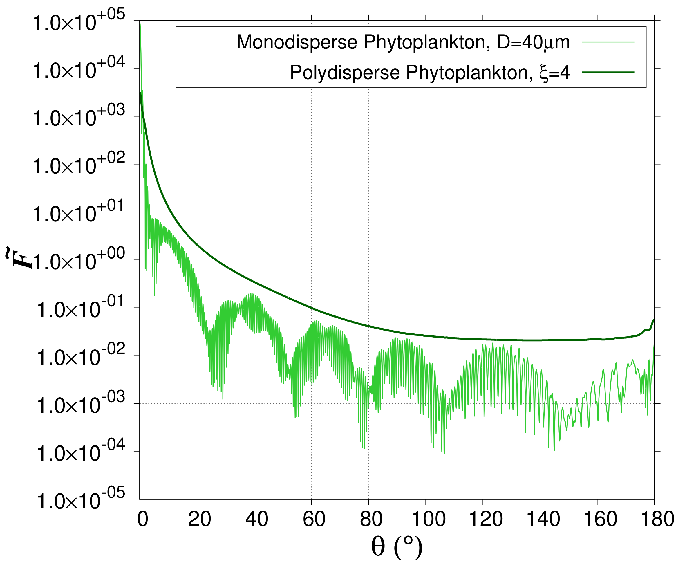
Section 2). Due to the sharp increase of the normalized phase function in the forward scattering directions (Figure 3), the selection of the relevant angular step for the numerical integration is crucial. For that purpose, the impact of angular step ( Δ θ ) on the calculation of b p θ a ˜ is studied using Lorentz-Mie simulations in DS1 (Figure 1, NoM2, M3). The normalized phase function of polydisperse particles F ˜ ( θ ) exhibits a maximum around θ = 0o [26]. For small ξ value, that is when the proportion of large-sized particles compared to smaller particles increases, the forward peak is sharper. Indeed, for particles with a large diameter as compared to the wavelength, F ˜ ( D , θ ) displays a sharp forward peak [26] due the concentration of light near θ = 0o caused by diffraction. The presence of the peak in F ˜ ( θ ) 
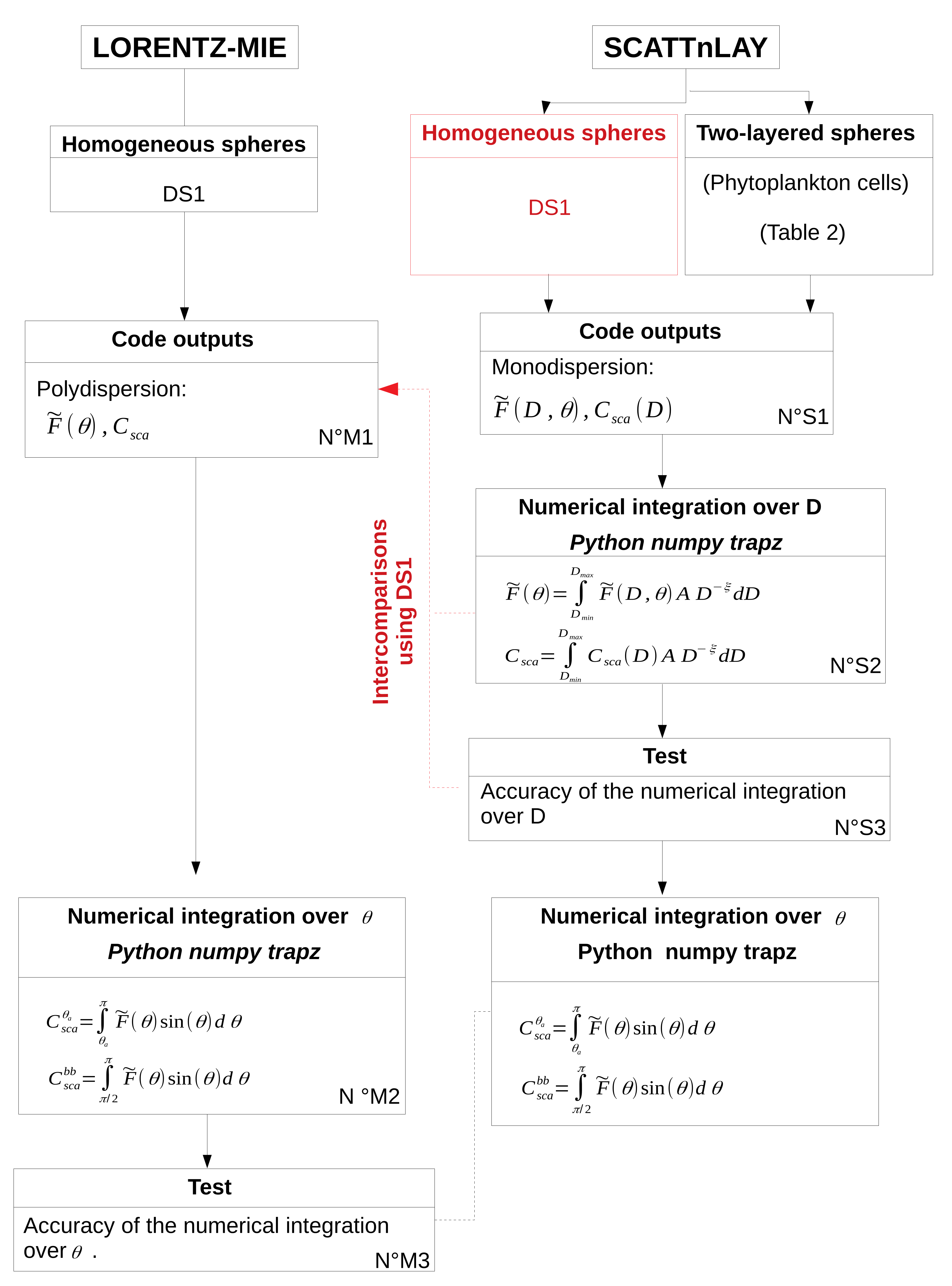
requires several integration points large enough to provide the desired numerical accuracy. The numerical integration over θ (Figure 1, NoM2) is performed using the “Trapz” function from the Numpy package with Python. The “Trapz” function performs an integration along the given axis using the composite trapezoidal rule. To test the accuracy of the integration and to find the correct integration step, Δ θ , we compare the result of the numerical integration of F ˜ ( θ ) between 0 and π to its theoretical value (=2) (Figure 1, NoM3). When Δ θ = 0.05o, corresponding to a total number of integration steps (N θ ) of 3600, the numerical integration value of F ˜ ( θ ) is in the range [1.999–2.000] for small ξ . For larger ξ , it is in the range [1.800–1.999]. When the value of the numerical integration is in the range [1.800–1.999], a renormalization factor is applied to F ˜ ( θ ) to ensure that the result of the numerical integration is exactly 2. We could also increase the number of integration points, but it would increase the computation time. Using a renormalization factor for large ξ is a good compromise to guarantee the accuracy and save computation time.
For two-layered spheres (i.e., phytoplankton cells), the ScattnLay code provides only normalized phase functions for monodisperse particles (Figure 1, NoS1), so the numerical integration over the particle diameter range (Equation (2)) is realized as a separate calculation with the Python “Trapz” function (Figure 1, NoS2). For monodisperse particles, the normalized phase function displays a forward peak as explained above but can also display a sequence of maxima and minima due to interference and resonance features [26,42]. The frequency of the maxima and minima over the range of θ increases with both increasing n r and size parameter (= π D / λ ). To test the accuracy of the numerical integration over the particle diameter range (Figure 1, NoS3), we ran the ScattnLay code for DS1 case studies and compared F ˜ ( θ ) and C s c a rebuilt from Equation (2) with Lorentz-Mie computations as the Lorentz-Mie code provides the polydisperse phase functions and cross section as outputs (Figure 1, NoM1). Note that even a narrow polydispersion washes out the interference and resonance features, which explains why most natural particulate assemblages do not exhibit such patterns [26,42] (Figure 3). A perfect match is obtained between the ScattnLay-rebuilt-polydisperse and Lorentz-Mie-polydisperse F ˜ ( θ ) and C s c a values when the integration step ( Δ D ) is set to 0.01 μ m for D in the range [0.03, 2 μ m]; 0.1 μ m for D in the range [2, 20 μ m]; 2.0 μ m for D in the range [20, 200 μ m]; and 10.0 μ m for D in the range [200, 500 μ m].
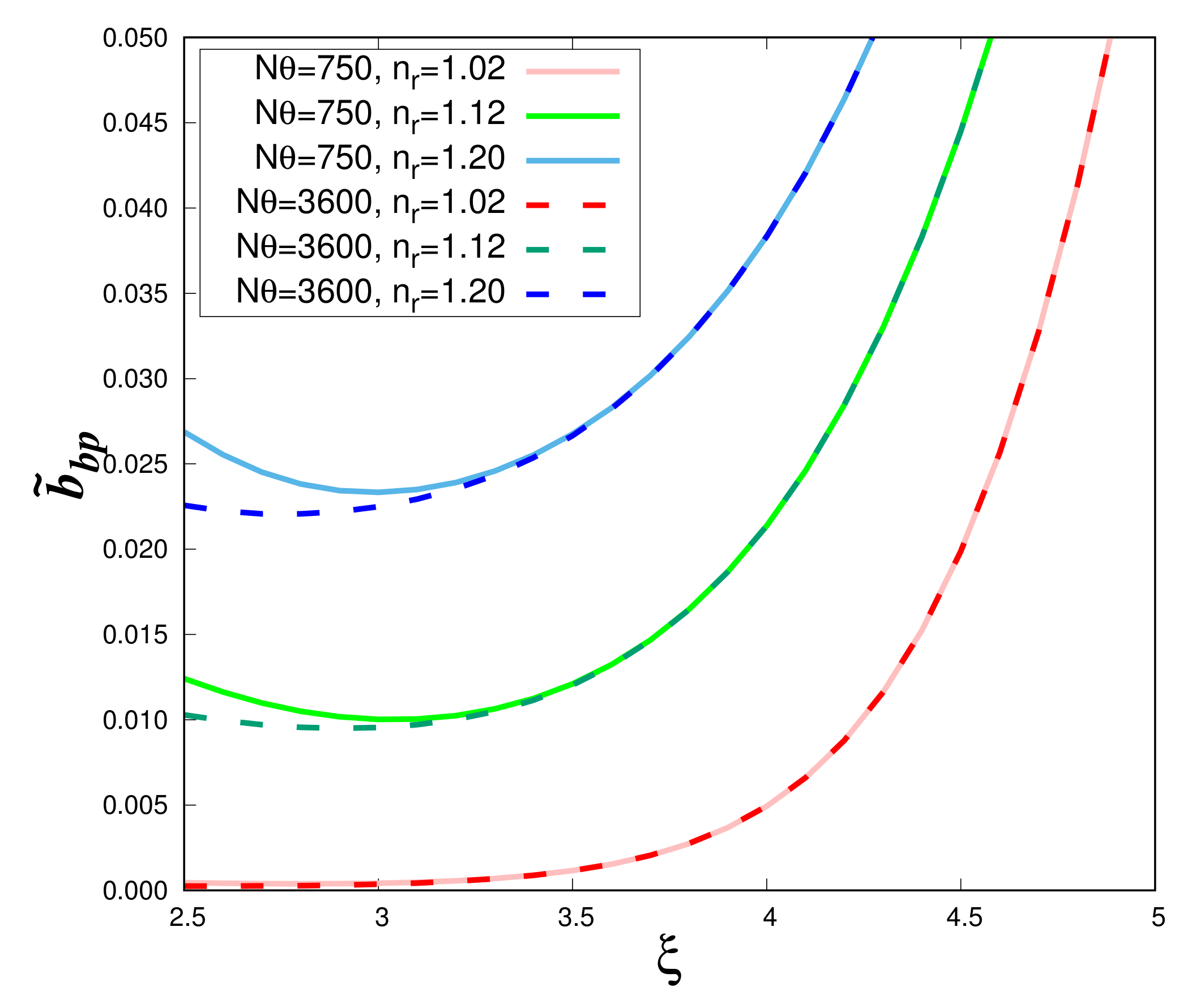
Using the DS1 data set, the impact of the angular integration on the backscattering ratio b b p θ a ˜ is examined as a function of the hyperbolic slope ξ for different values of the real refractive index and two values of total angular steps (i.e., N θ = 750 and 3600) (Figure 4). The impact of the integration is noticeable only for ξ values lower than about 3 and relatively high n r values. When the number of angular steps increases, the curves become flatter at low ξ values. Differences in the curve shape are reduced if we increase the angular step. For Δ θ = 0.24o (N θ = 750), the present results of the Lorentz-Mie calculations (solid lines in Figure 4) perfectly match those previously obtained by Twardowski et al. [5] (not shown). However, in this case (N θ = 750), the numerical integration is not accurate enough as the integration of Equation (1) gives values between 1.999 ( ξ = 4.9) and 1.04 ( ξ = 2.5 ). In the following, Δ θ is set to 0.05o (N θ = 3600) and Figure 4 (dashed lines) will be the reference figure for homogeneous spheres.

5.2. Impact of the Structural Heterogeneity of Phytoplankton Cells on the Bulk Particulate Backscattering Ratio

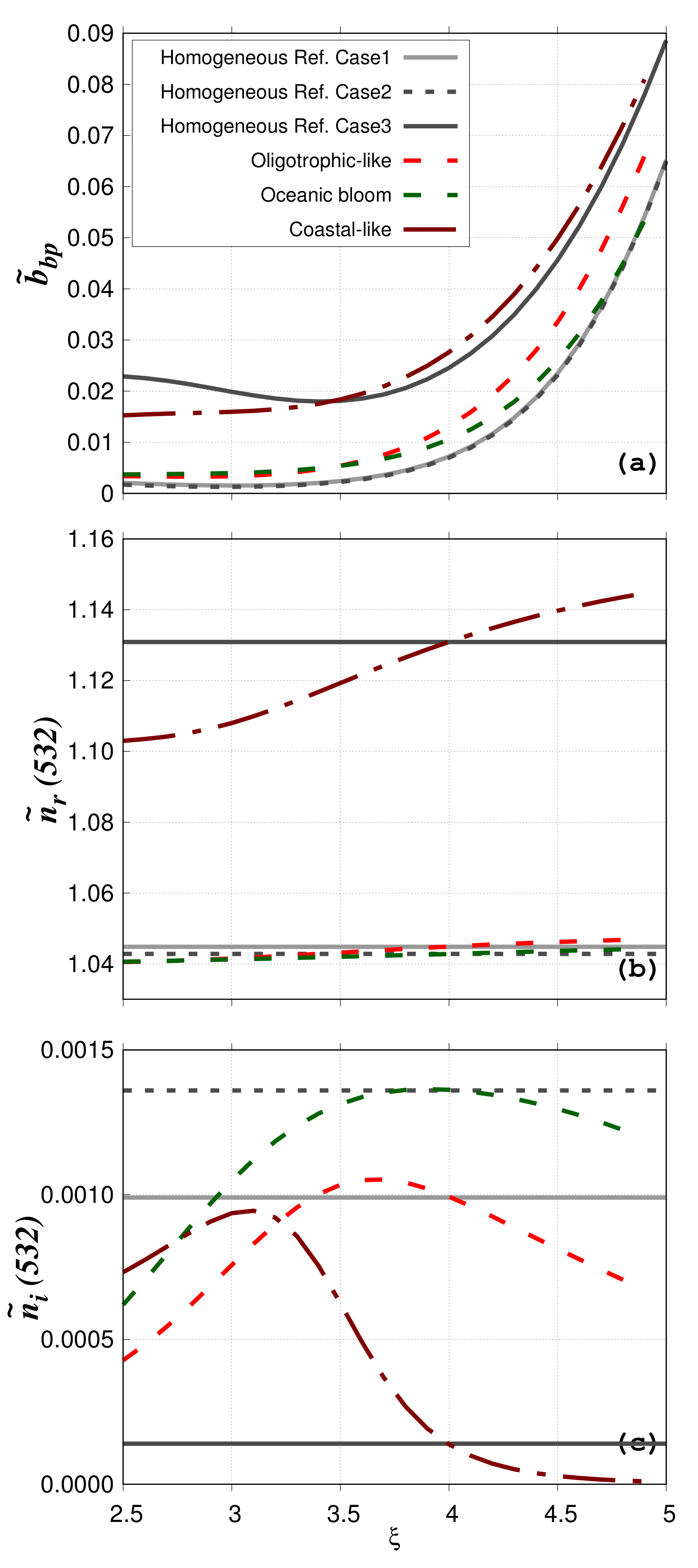
The impact of phytoplankton cell structural heterogeneity on b b p θ a ˜ is examined as a function of ξ for the three previously described water bodies (oligotrophic-like, phytoplankton bloom, coastal-like) considering the 80%–20% phytoplankton morphological model (Figure 5a). The real and imaginary bulk refractive indices for oligotrophic-like, phytoplankton bloom, and coastal-like case studies, vary with ξ as the relative proportions of the different particle components, having different n r and n i , vary with ξ (Table 1, Table 2, Table 3, Table 4 and Table 5 and Figure 5b,c). For the no-mineral water bodies (oligotrophic-like and phytoplankton bloom), n r ˜ stays around 1.04 ± 0.007 (Figure 5b). In contrast, n i ˜ shows large variation with ξ for both oligotrophic-like and phytoplankton bloom water bodies (Figure 5c). In bloom conditions, n i ˜ increases as the relative proportion of phytoplankton increases as compared to the no bloom conditions. In agreement with typical values of the oceanic bulk imaginary refractive index [43], the n i ˜ values for the particulate populations considered here are always lower than 0.002. In the presence of mineral particles (coastal-like), n r ˜ increases as MIN have a higher n r than VIR, BAC, PHY and DET. Its values are between 1.103 ( ξ = 2.5 ) and 1.145 ( ξ = 4.9 ). Values of n i ˜ vary between 9.79 × 10 6 and 9.44 × 10 4 .
The impact of the structural heterogeneity of phytoplankton cells is evaluated by comparison with Lorentz-Mie calculations (particulate assemblages composed of homogeneous spheres only, regardless of the particle group) performed for low and high bulk refractive index. These case studies with homogeneous spheres only are named “Homogeneous reference cases”. The real and imaginary values of the bulk refractive indices are 1.045 and 9.93 × 10 4 for the “Homogeneous reference case 1”, 1.043 and 1.36 × 10 3 for the “Homogeneous reference case 2”, and 1.131 and 1.37 × 10 4 for the “Homogeneous reference case 3”, respectively (Figure 5b,c). These values of n r ˜ and n i ˜ were chosen to be equal to values of n r ˜ and n i ˜ obtained for the oligotrophic-like, phytoplankton bloom, and the coastal-like case study when ξ = 4. “Homogeneous reference cases 1 and 2” with low n r ˜ represent phytoplankton-dominated Case 1 waters and are compared with the oligotrophic-like and phytoplankton bloom water body, respectively. “Homogeneous reference case 3” with high n r ˜ represents mineral-dominated Case 2 waters and is compared with the coastal-like water body. The variation of b b p θ a ˜ due to structural heterogeneity of phytoplankton cells is evaluated using the relative absolute difference calculated between the homogeneous reference cases (named x in Equation (13)) and oligotrophic, phytoplankton bloom or coastal-like water bodies (named y in Equation (13)):
Δ ϵ = | x y | ( x + y ) × 200 ( % )
Even if the numerical relative abundance of phytoplankton is very small for the oligotrophic-like water body (=8.4 × 10 3 %), the structural heterogeneity increases the b b p θ a ˜ value by 58% compared to the homogeneous case (“Homogeneous reference case 1”). This is consistent with previous studies showing the large contribution of coated spheres to the backscattering signal [15,16,18,19,22,44]. The value of Δ ϵ calculated between the oligotrophic-like and phytoplankton bloom water bodies is smaller (=22% at ξ = 4) even if n i ˜ is different (9.93 × 10 4 for oligotrophic-like against 1.36 × 10 3 for phytoplankton bloom). This latter pattern provides evidence that the structural heterogeneity (coated-sphere model) has a greater impact on the particulate backscattering ratio than the tested increase in the bulk imaginary refractive index. The relative absolute differences between the phytoplankton bloom and “Homogeneous reference case 2” is 41%. When mineral particles are taken into account, Δ ϵ is 12% between the “Homogeneous reference case 3” and the coastal-like water body. This smaller difference is because phytoplankton have a smaller impact on the bulk scattering when highly scattering particles such as minerals are added.
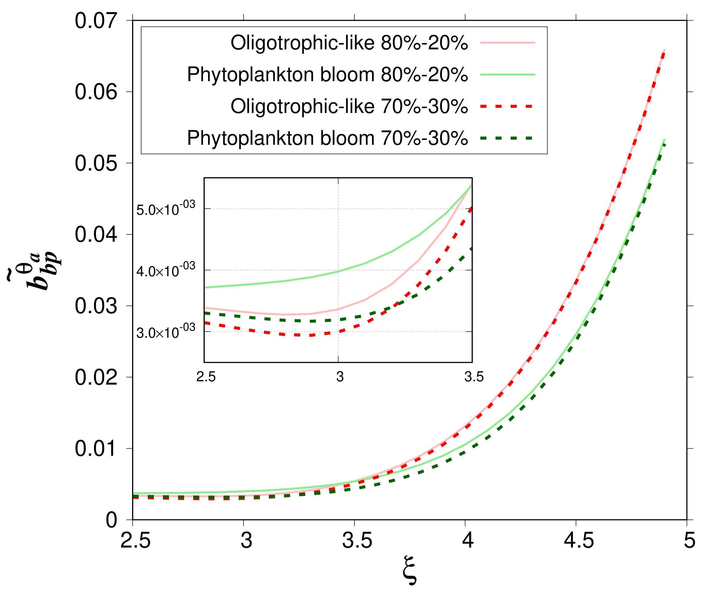
The impact of the relative volume of the cytoplasm on b b p θ a ˜ is now evaluated by comparing the change of b b p θ a ˜ as a function of ξ for the 80%–20% and 70%–30% models for the oligotrophic-like and phytoplankton bloom water bodies (Figure 6). The mean relative difference in b b p θ a ˜ is about 5.41% with a maximum value of 11.5 % ( ξ = 3) for oligotrophic-like case study. In bloom conditions, the mean relative difference reaches 13.0% with a maximum value of 23.5% ( ξ = 3.2). 
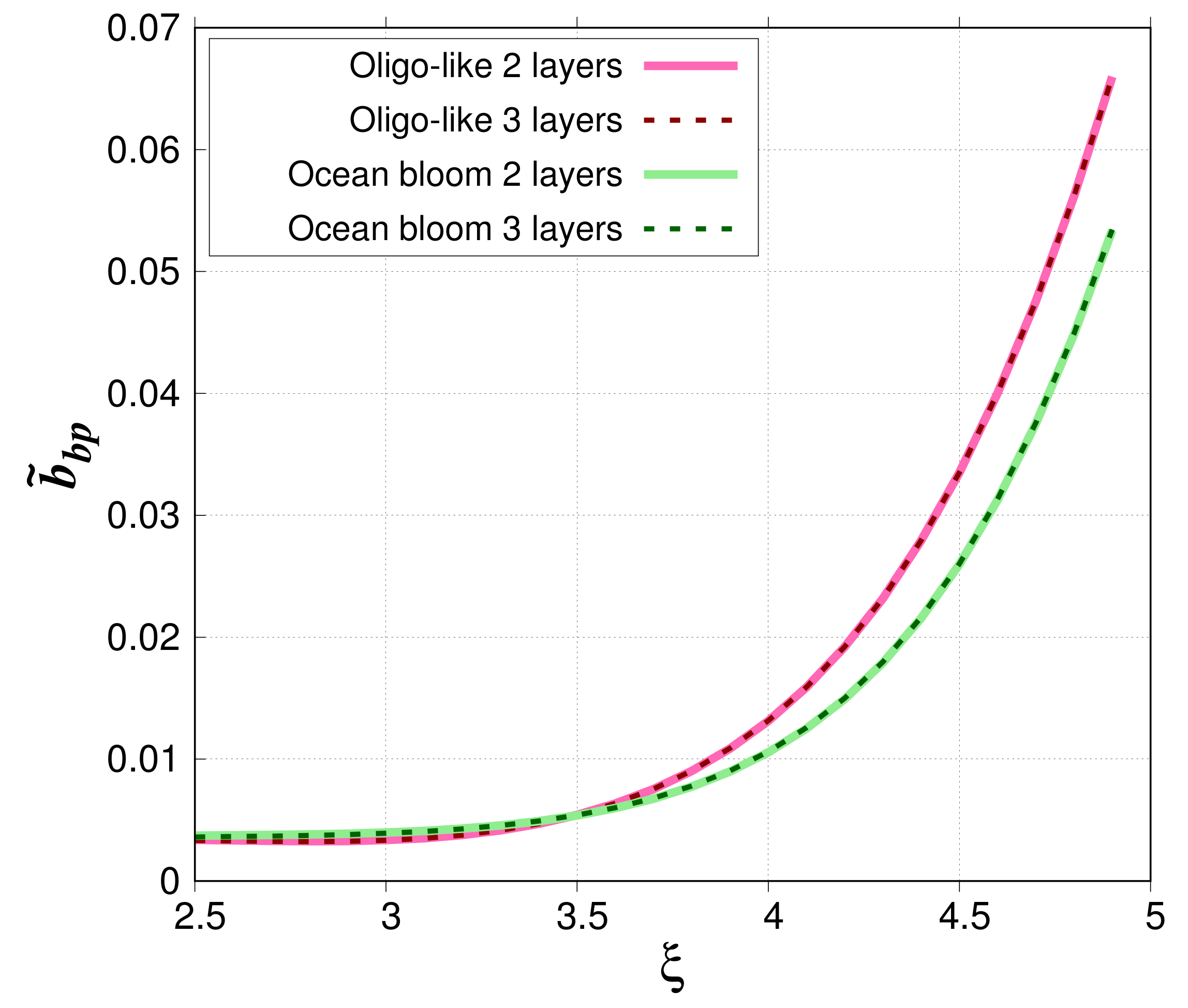
Figure 7 compares simulated b b p θ a ˜ when phytoplankton cells are modeled as two-layered spheres (80%–20%) or three-layered spheres (80%–18.5%–1.5%). For the oligotrophic-like waters, relative absolute differences are small. They range between 0.0174% and 1.81% with a mean value of 0.444%. For phytoplankton bloom case study, they are between 9.84 × 10 3 and 2.86% with a mean value of 0.894%.
Regardless of the morphological model used to optically simulate phytoplankton cells, the b b p θ a ˜ reaches an asymptote when ξ decreases for phytoplankton bloom water bodies ( b b p θ a ˜ = 0.005 for ξ = 3.5 and 0.004 for ξ = 2.5). The value of the asymptote is consistent with previous observations [5], which showed the lowest backscattering ratio (about 0.005) in waters with high chlorophyll-a concentration.
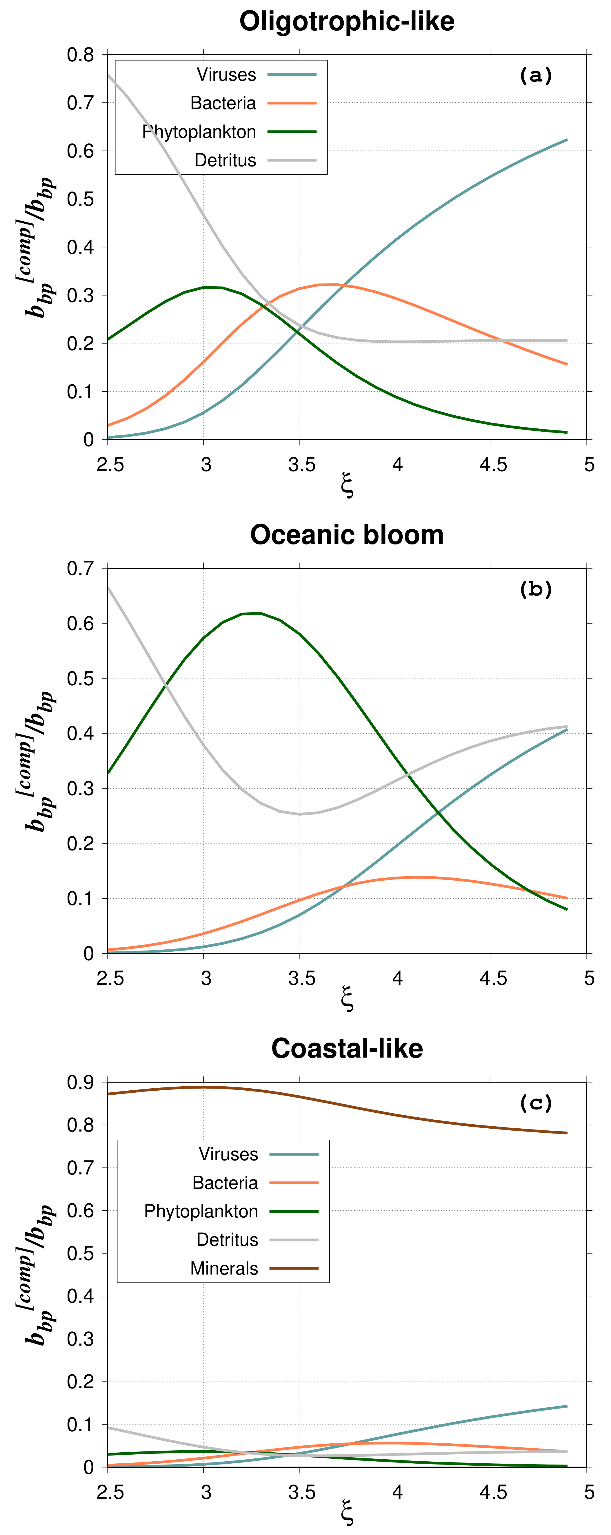
The contribution of the different particle groups to the backscattering ratio is presented in Figure 8 for the 80%–20% model and ξ = 4. For coastal-like waters, the minerals contribute more than 80% of the total b b p θ a ˜ , whereas they contribute only 6.5% to the total particulate abundance. This percentage agrees with the results of Stramski et al. [25] (Figure 12 in their paper). Such high contribution to backscattering is due to the high real refractive index of minerals. As in Stramski et al. [25], these results show the important role of minerals even when they are less abundant than organic living and non-living particles. In oligotrophic-like waters, the contribution of heterotrophic bacteria ranges from a few to about 30% with a maximum for ξ between 3.5 and 4, which agrees with Stramski and Kiefer [24]. The contribution of viruses is quite high, about 40–60% for ξ between 4 and 5. This high contribution is explained by the extreme value of viral abundance (around 1 × 10 14 particles per cubic meter) used in this study [24]. As for bacteria, the contribution of phytoplankton ranges between a few and 30% with a maximum around ξ = 3. For a ξ 
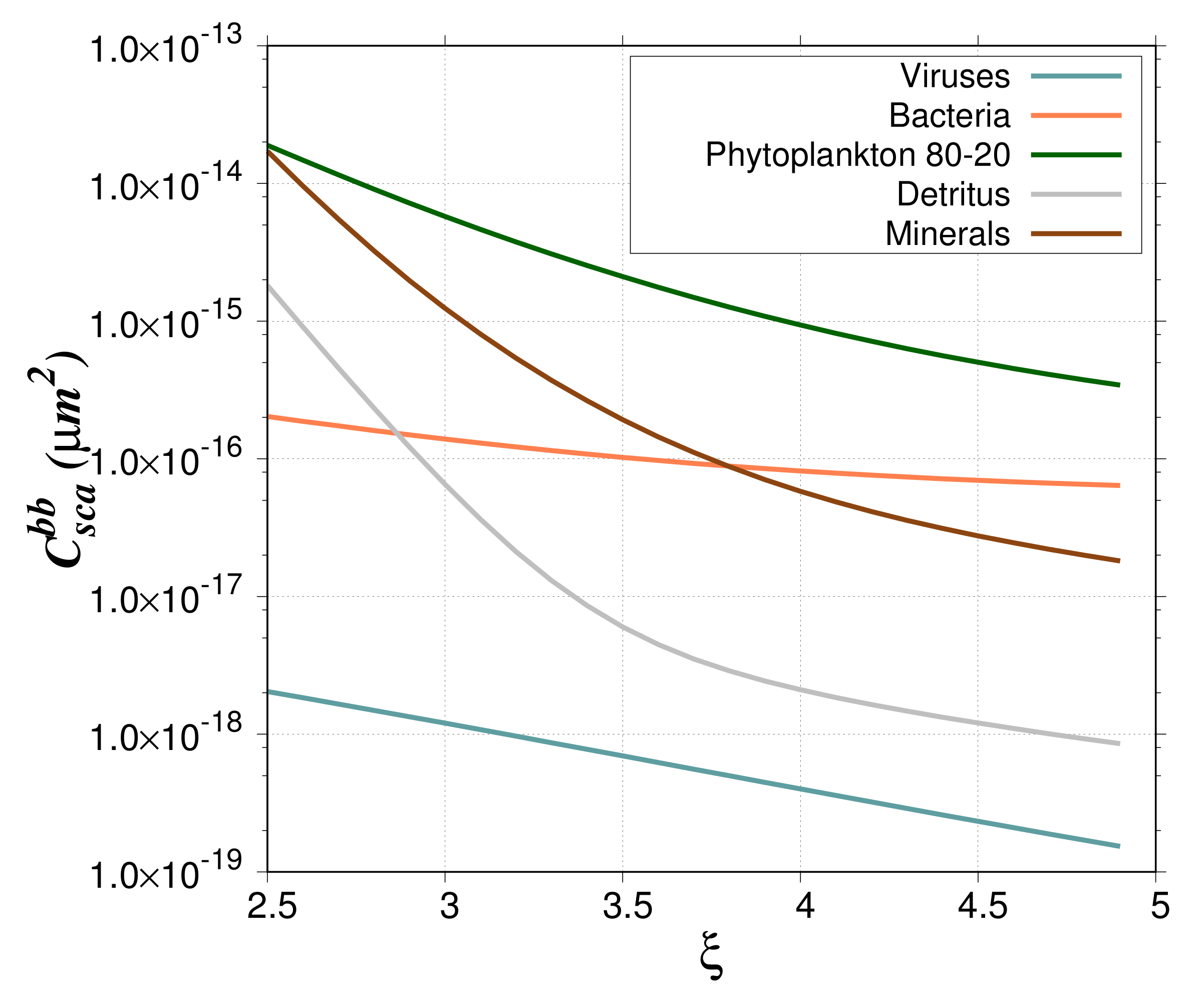
value of 4, typical of oligotrophic waters, the contribution is around 10%. For the phytoplankton bloom study case, the contribution of phytoplankton cells is between 10% and 60%; maximum values are reached for a PSD slope between 3 and 3.5. Such high percentages are due to the higher backscattering cross section of phytoplankton as compared to the other particles (Figure 9). The low phytoplankton abundance is offset by the high C s c a , P H Y b b so that the backscattering coefficient of phytoplankton represents a significant contribution to the total backscattering.

6. Concluding Remarks

Modeling phytoplankton cells as two-layered spheres tends to increase the bulk backscattering ratio because heterogeneous spheres are more efficient backscatterers. Even if the phytoplankton component has the smallest relative abundance, its impact on b b p θ a ˜ can be important depending on the hyperbolic slope of the Junge distribution. This is because phytoplankton cells have the highest backscattering cross section. For ξ = 4, the relative difference (in absolute value), ( Δ ϵ ), between b b p θ a ˜ for the oligotrophic-like and the reference case, having the same bulk refractive index but composed exclusively of homogeneous spheres, can reach about 58%. When minerals are added, the impact of phytoplankton decreases as the scattering by minerals dominates.
Considering different sub-populations of particles with different refractive index implies that the bulk refractive index varies with the value of the hyperbolic slope of the PSD, as the contribution of each scattering component varies. Consequently, the development of models, similar to the one proposed by Twardowski et al. [5] to derive n r ˜ from b b p θ a ˜ and ξ , but accounting for phytoplankton heterogeneity, is not straightforward. Other aspects of the problem and other parameters such as the adoption of a 2D or 3D model, the proportion between cytoplasm and chloroplast, or the variation of phytoplankton refractive index according to the considered species, would have to be taken into account. One option would be to develop a look-up table approach based on the main parameters driving the b b p θ a ˜ variability. For that purpose, other simulations would have to be performed to be able to identify the pertinent parameters.
In this study, a large set of numerical simulations, as well as a proper methodology have been developed to simulate the particulate scattering properties of a water body in its complexity. We show that a special care should be taken in the integration step size when the particulate scattering coefficients are calculated from the particulate scattering function, especially for relatively small values of the PSD slope. We show that an integration angular step of 0.05o (N θ = 3600) is required to obtain the required accuracy considering the inputs (refractive indices and size range) used in this study.
The method is adapted to be used repeatedly to model a very large variety of particulate assemblages. While the present study has been limited to three case studies, additional calculations can be conducted to better represent the variability encountered in oceanic environments in terms of particulate community and its complexity in terms of mixing, morphology, size, and chemical nature.
For example, in waters with significant presence of specific populations of phytoplankton or under bloom conditions, the Junge-like approximation of PSD is usually unsatisfactory [36,37,38,45]. We also showed that the relative volume of the model chloroplast to the cytoplasm or the presence of third layer to model the cell wall can all affect the backscattering ratio (about 5–25%). It means that changes in the phytoplankton structural heterogeneity can explain partly the natural variability of the backscattering ratio, particularly in bloom conditions.
Further work is required, mainly experimental studies, to better characterize the internal structure and chemical composition of viruses, heterotrophic bacteria, biogenic detritus, and particle aggregates. This will allow, as Robertson Lain et al. [23] did for phytoplankton, suitable models to be developed to describe properly, in numerical code, the morphological properties of various types of particles to provide more realistic simulations of their optical properties.

Author Contributions

The research is completed through collaboration of all authors. L.D.-G. and H.L. were the team leaders of this work who were responsible for coordination. D.D. was in charge of program coding and assisted in data analysis. W.M. was involved in discussions. L.D.-G. analyzed the data and wrote the paper.

Funding

The authors gratefully acknowledge the support from the French Space Agency (CNES) through the COYOTE project (CNES/TOSCA program).

Acknowledgments

The authors thank Michael Twardowski, (Harbor Branch Oceanographic Institute) for the valuable advice. We appreciate thoughtful comments from the anonymous reviewers and Dariusz Stramski, who provided time and effort to improve this manuscript. Experiments presented in this paper were carried out using the CALCULCO computing platform, supported by SCoSI/ULCO (Service COmmun du Système d’Information de l’Université du Littoral Côte d’Opale).

Conflicts of Interest

The authors declare no conflict of interest.

References

  1. Preisendorfer, R.W. Hydrologic Optics, Volume 1: Introduction; Springfield National Technical Information Service; Office of Naval Research: Arlington, VA, USA, 1976. [Google Scholar]
  2. Morel, A. The Scattering of Light by Seawater: Experimental Results and Theoretical Approach; Translation by George Halikas of the paper published in French in AGARD Lecture Series; No61; North Atlantic Treaty Organization: Neuilly-sur-Seine, France, 1973. [Google Scholar]
  3. Boss, E.; Pegau, W.S.; Gardner, W.D.; Zaneveld, J.R.V.; Barnard, A.H.; Twardowski, M.S.; Chang, G.C.; Dickey, T.D. The spectral particulate attenuation and particle size distribution in the bottom boundary layer of a continental shelf. J. Geophys. Res. 2001, 106, 9509–9516. [Google Scholar] [CrossRef]
  4. Boss, E.; Twardowski, M.S.; Herring, S. Shape of the particulate beam attenuation spectrum and its relation to the size distribution of oceanic particles. Appl. Opt. 2001, 40, 4885–4893. [Google Scholar] [CrossRef] [PubMed]
  5. Twardowski, M.; Boss, E.; Macdonald, J.; Pegau, W.; Barnard, A.; Zaneveld, J. A model for estimating bulk refractive index from optical backscattering ratio and the implications for understanding particle composition in case I and case II waters. J. Geophys. Res. 2001, 106, 14129–14142. [Google Scholar] [CrossRef]
  6. Boss, E.; Pegau, W.S.; Lee, M.; Twardowski, M.; Shybanov, E.; Korotaev, G.; Baratange, F. Particulate backscattering ratio at LEO 15 and its use to study particle composition and distribution. J. Geophys. Res. 2004, 109, C01014. [Google Scholar] [CrossRef]
  7. Loisel, H.; Mériaux, X.; Berthon, J.F.; Poteau, A. Investigation of the optical backscattering to scattering ratio of marine particles in relation to their biogeochemical composition in the eastern English Channel and southern North Sea. Limnol. Oceanogr. 2007, 52, 739–752. [Google Scholar] [CrossRef] [Green Version]
  8. Nasiha, H.J.; Shanmugam, P. Estimating the Bulk Refractive Index and Related Particulate Properties of Natural Waters from Remote-Sensing Data. IEEE J. Sel. Top. Appl. Earth Obs. Remote Sens. 2015, 8, 5324–5335. [Google Scholar] [CrossRef]
  9. Snyder, W.A.; Arnone, R.A.; Davis, C.O.; Goode, W.; Gould, R.W.; Ladner, S.; Lamela, G.; Rhea, W.J.; Stavn, R.; Sydor, M.; et al. Optical scattering and backscattering by organic and inorganic particulates in U.S. coastal waters. Appl. Opt. 2008, 47, 666–677. [Google Scholar] [CrossRef]
  10. Sullivan, J.; Twardowski, M.; Donaghay, P.; Freeman, S. Use of optical scattering to discriminate particle types in coastal waters. Appl. Opt. 2005, 44, 1667–1680. [Google Scholar] [CrossRef]
  11. Meyer, R.A. Light scattering from biological cells: Dependence of backscatter radiation on membrane thickness and refractive index. Appl. Opt. 1979, 18, 585–588. [Google Scholar] [CrossRef]
  12. Bricaud, A.; Zaneveld, J.R.V.; Kitchen, J.C. Backscattering efficiency of coccolithophorids: Use of a three-layered sphere model. Proc. SPIE 1992, 1750, 27–33. [Google Scholar]
  13. Kitchen, J.C.; Zaneveld, J.R.V. A three-layered sphere model of the optical properties of phytoplankton. Limnol. Oceanogr. 1992, 37, 1680–1690. [Google Scholar] [CrossRef] [Green Version]
  14. Stramski, D.; Piskozub, J. Estimation of scattering error in spectrophotometric measurements of light absorption by aquatic particles from three-dimensional radiative transfer simulations. Appl. Opt. 2003, 42, 3634–3646. [Google Scholar] [CrossRef]
  15. Moutier, W.; Duforêt-Gaurier, L.; Thyssen, M.; Loisel, H.; Mériaux, X.; Courcot, L.; Dessailly, D.; Rêve, A.H.; Grégori, G.; Alvain, S.; et al. Evolution of the scattering properties of phytoplankton cells from flow cytometry measurements. PLoS ONE 2017, 12. [Google Scholar] [CrossRef] [PubMed]
  16. Poulin, C.; Zhang, X.; Yang, P.; Huot, Y. Diel variations of the attenuation, backscattering and absorption coefficients of four phytoplankton species and comparison with spherical, coated spherical and hexahedral particle optical models. J. Quant. Spectrosc. Radiat. Transf. 2018, 217, 288–304. [Google Scholar] [CrossRef]
  17. Quirantes, A.; Bernard, S. Light scattering by marine algae: Two-layer spherical and nonspherical models. J. Quant. Spectrosc. Radiat. Transf. 2004, 89, 311–321. [Google Scholar] [CrossRef]
  18. Vaillancourt, R.D.; Brown, C.W.; Guillard, R.L.; Balch, W.M. Light backscattering properties of marine phytoplankton: Relationships to cell size, chemical composition and taxonomy. J. Plankton Res. 2004, 26, 191–212. [Google Scholar] [CrossRef]
  19. Volten, H.; Haan, J.F.; Hovenier, J.W.; Schreurs, R.; Vassen, W.; Dekker, A.G.; Hoogenboom, H.J.; Charlton, F.; Wouts, R. Laboratory measurements of angular distributions of light scattered by phytoplankton and silt. Limnol. Oceanogr. 1998, 43, 1180–1197. [Google Scholar] [CrossRef] [Green Version]
  20. Witkowski, K.; Król, T.; Zielinski, A.; Kuten, E. A light-scattering matrix for unicellular marine phytoplankton. Limnol. Oceanogr. 1998, 43, 859–869. [Google Scholar] [CrossRef] [Green Version]
  21. Stramski, D.; Boss, E.; Bogucki, D.; Voss, K.J. The role of seawater constituents in light backscattering in the ocean. Prog. Oceanogr. 2004, 61, 27–56. [Google Scholar] [CrossRef]
  22. Whitmire, A.L.; Pegau, W.S.; Karp-Boss, L.; Boss, E.; Cowles, T.J. Spectral backscattering properties of marine phytoplakton cultures. Opt. Express 2010, 18, 15073–15093. [Google Scholar] [CrossRef]
  23. Robertson Lain, L.; Bernard, S.; Evers-King, H. Biophysical modelling of phytoplankton communities from first principles using two-layered spheres: Equivalent Algal Populations (EAP) model. Opt. Express 2014, 22, 16745–16758. [Google Scholar] [CrossRef] [PubMed]
  24. Stramski, D.; Kiefer, D.A. Light scattering by microorganisms in the open ocean. Prog. Oceanogr. 1991, 28, 343–383. [Google Scholar] [CrossRef]
  25. Stramski, D.; Bricaud, A.; Morel, A. Modeling the inherent optical properties of the ocean based on the detailed composition of the planktonic community. Appl. Opt. 2001, 40, 2929–2945. [Google Scholar] [CrossRef] [PubMed]
  26. Mishchenko, M.I.; Travis, L.D.; Lacis, A.A. Scattering, Absorption and Emission of Light of Small Particles; Cambridge University Press: Cambridge, UK, 2002; ISBN 9780521782524. [Google Scholar]
  27. Jonasz, M. Particle size distribution in the Baltic. Tellus 1983, B35, 346–358. [Google Scholar] [CrossRef]
  28. Loisel, H.; Nicolas, J.M.; Sciandra, A.; Stramski, D.; Poteau, A. Spectral dependency of optical backscattering by marine particles from satellite remote sensing of the global ocean. J. Geophys. Res. 2006, 111, C09024. [Google Scholar] [CrossRef]
  29. Morel, A.; Bricaud, A. Inherent optical properties of algal cells, including picoplankton. Theoretical and experimental results. Can. Bull. Fish. Aquat. Sci. 1986, 214, 521–559. [Google Scholar]
  30. Boss, E.; Slade, W.H.; Behrenfeld, M.; Dall’Olmo, G. Acceptance angle effects on the beam attenuation in the ocean. Opt. Express 2009, 17. [Google Scholar] [CrossRef]
  31. Dolman, V.L. Meerhoff Mie Program User Guide; Internal Report Astronomy Department, Free University: Amsterdam, The Netherlands, 1989. [Google Scholar]
  32. Peña, O.; Pal, U. Scattering of electromagnetic radiation by a multilayered sphere. Comput. Phys. Commun. 2009, 180, 2348–2354. [Google Scholar] [CrossRef]
  33. Yang, W. Improved recursive algorithm for light scattering by a multilayered sphere. Appl. Opt. 2003, 42, 1710–1720. [Google Scholar] [CrossRef]
  34. Aas, E. Refractive index of phytoplankton derived from its metabolite composition. J. Plankton Res. 1996, 18, 2223–2249. [Google Scholar] [CrossRef] [Green Version]
  35. Buonassissi, C.J.; Dierssen, H.M. A regional comparison of particle size distributions and the power law approximation in oceanic and estuarine surface waters. J. Geophys. Res. 2010, 115, C10028. [Google Scholar] [CrossRef]
  36. Reynolds, R.A.; Stramski, D.; Wright, V.M.; Woźniak, S.B. Measurements and characterization of particle size distributions in coastal waters. J. Geophys. Res. 2010, 115, C08024. [Google Scholar] [CrossRef]
  37. Reynolds, R.A.; Stramski, D.; Neukermans, G. Optical backscattering by particles in Arctic seawater and relationships to particle mass concentration, size distribution, and bulk composition. Limnol. Oceanogr. 2016, 61, 1869–1890. [Google Scholar] [CrossRef] [Green Version]
  38. Woźniak, S.B.; Stramski, D.; Stramska, M.; Reynolds, R.A.; Wright, V.M.; Miksic, E.Y.; Cichocka, M.; Cieplak, A.M. Optical variability of seawater in relation to particle concentration, composition, and size distribution in the nearshore marine environment at Imperial Beach, California. J. Geophys. Res. 2010, 115, C08027. [Google Scholar] [CrossRef]
  39. Middleboe, M.; Brussaard, C.P.D. Marine Viruses: Key Players in Marine Ecosystems. Viruses 2017, 9, 302. [Google Scholar] [CrossRef] [PubMed]
  40. Brotas, V.; Brewin, R.; Sá, C.; Brito, A.C.; Silva, A.; Mendes, C.R.; Diniz, T.; Kaufmann, M.; Tarran, G.; Groom, S.B.; et al. Deriving phytoplankton size classes from satellite data: Validation along a trophic gradient in the eastern Atlantic Ocean. Remote Sens. Environ. 2013, 134, 66–77. [Google Scholar] [CrossRef]
  41. Brewin, R.J.W.; Sathyendranath, S.; Hirata, T.; Lavender, S.; Barciela, R.M.; Hardman-Mountford, N.J. A three-component model of phytoplankton size class for the Atlantic Ocean. Ecol. Model. 2010, 221, 1472–1483. [Google Scholar] [CrossRef]
  42. Mishchenko, M.; Lacis, A. Manifestations of morphology-dependent resonances in Mie scattering matrices. Appl. Math. Comput. 2000, 116, 167–179. [Google Scholar] [CrossRef]
  43. Bricaud, A.; Roesler, C.; Zaneveld, J.R.V. In situ methods for measuring the inherent optical properties of ocean waters. Limnol. Oceanogr. 1995, 40, 393–410. [Google Scholar] [CrossRef] [Green Version]
  44. Zaneveld, J.R.V.; Kitchen, J.C. The variation in the inherent optical properties of phytoplankton near an absorption peak as determined by various models of cell structure. J. Geophys. Res. 1995, 100, 309–313. [Google Scholar] [CrossRef]
  45. Reynolds, R.A.; Stramski, D.; Mitchell, B.G. A chlorophyll-dependent semianalytical reflectance model derived from field measurements of absorption and backscattering coefficients within the Southern Ocean. J. Geophys. Res. 2001, 106, 7125–7138. [Google Scholar] [CrossRef] [Green Version]
Figure 1. Flow chart of the integration procedure applied to the MIE and ScattnLay outputs.
Applsci 08 02689 g001
Figure 2. Composite PSD as derived from individual PSDs of the five considered particle groups for (a) the oligotrophic-like water body and (b) the phytoplankton bloom water body. N T O T = 1.1262 × 10 14 particles per m 3 and ξ = 4.
Applsci 08 02689 g002
Figure 3. Interference and resonance features observed for the scattering phase function of monodisperse particles (light green). The major low-frequency maxima and minima are called the “interference structure”. The high-frequency ripples are resonance features. The interference and resonance feature are washed out for a polydisperse assemblage of particles (dark green).
Applsci 08 02689 g003
Figure 4. Results of Lorentz-Mie calculations (DS1) of the particulate backscattering ratio b b p θ a ˜ as a function of the hyperbolic slope, ξ , and different values of n r and N θ . The imaginary part of the refractive index = 0.005 as in Twardowski et al. [5]. This figure can be compared to Figure 1 in Twardowski et al. [5].
Applsci 08 02689 g004
Figure 5. (a) Particulate backscattering ratio b b p θ a ˜ as a function of the hyperbolic slope for the oligotrophic-like (red dashed line), phytoplankton bloom (green dashed line), and coastal-like (brown dashed line) water bodies as described in Section 4. Black and gray lines are for homogeneous reference cases. The gray solid line corresponds to n r = 1.045, n i = 9.93 × 10 4 , the black dashed line to n r = 1.1043, n i = 1.36 × 10 3 , and the black solid line to n r = 1.131, n i = 1.37 × 10 4 , respectively. Phytoplankton cells are modeled as two-layered spheres with a relative volume of the cytoplasm of 20% (%cyt-%chl = 80–20). (b) as in panel (a) but for the real refractive index. (c) as in panel (a) but for the imaginary part of the refractive index.
Applsci 08 02689 g005
Figure 6. Particulate backscattering ratio as a function of the hyperbolic slope for oligotrophic-like and phytoplankton bloom water bodies. Phytoplankton cells are modeled as two-layered spheres with a relative volume of the chloroplast of 20 % and 30 %, as indicated.
Applsci 08 02689 g006
Figure 7. Particulate backscattering ratio as a function of the hyperbolic slope for oligotrophic-like and phytoplankton bloom water bodies. Phytoplankton cells are modeled as two-layered spheres (80%–20%) or three-layered spheres (80%–18.5%–1.5%), as indicated.
Applsci 08 02689 g007
Figure 8. Contribution of the different particle groups the total bulk backscattering ratio for (a) oligotrophic-like, (b) phytoplankton bloom, and (c) coastal-like water bodies. The phytoplankton cells are modeled as a two-layered sphere (80%–20%).
Applsci 08 02689 g008
Figure 9. Backscattering cross sections, C s c a b b , of the different particle groups. The phytoplankton cells are modeled as a two-layered sphere (80%–20%).
Applsci 08 02689 g009
Table 1. Summary of the seawater constituents.
Component (j)Sphere Model D min - D max ( μ m) n r n i
Viruseshomogeneous0.03–0.21.050
Heterotrophic bacteriahomogeneous0.2–21.051.0 × 10 4
Phytoplankton cellstwo or three-layered0.3–401.044 *1.5 × 10 3 *
Organic detritushomogeneous0.05–5001.042.3 × 10 5
Mineralshomogeneous0.05–5001.181.0 × 10 4
* the values represent the equivalent refractive indices (Equation (12)). The refractive indices of the spheres representing the chloroplast and cytoplast are described in Table 2. λ = 532 nm.
Table 2. Refractive index ( n r (chlp) + i n i (chlp)) of the sphere representing the chloroplast for two morphological models. The refractive index of the sphere representing the cytoplast is constant (1.02 + i 1.336 × 10 4 ). The equivalent refractive index of the cell is 1.044 + i 1.5 × 10 3 .
Model * (%cyt-%chlp)80%–20%70%–30%80%–18.5%–1.5%
n r 1.1401.1001.144
n i 6.966 × 10 3 4.688 × 10 3 7.531 × 10 3
* The percentages represent the relative volume of the model cytoplasm and chloroplast.
Table 3. Relative abundance of viruses (VIR), bacteria (BAC), phytoplankton (PHY), and organic detritus (DET) with the corresponding bulk refractive index (Equations (9) and (10)) for the water body with no bloom conditions and no minerals (oligotrophic-like).
Relative Abundance N j (%)
ξ n r ˜ n i ˜ VIRBACPHYDET
2.51.0404.280 × 10 4 78.855.3490.405915.39
31.0427.570 × 10 4 84.742.1200.100213.04
3.51.0431.034 × 10 3 88.500.82440.028110.64
41.0459.931 × 10 4 91.150.31780.00848.528
4.91.0476.718 × 10 4 94.355.651 × 10 2 0.00105.588
Table 4. Relative abundance of viruses (VIR), bacteria (BAC), phytoplankton (PHY), and organic detritus (DET) with the corresponding bulk refractive index (Equations (9) and (10)) for the water body with phytoplankton bloom conditions and no minerals (phytoplankton bloom).
Relative Abundance N j (%)
ξ n r ˜ n i ˜ VIRBACPHYDET
2.51.0416.195 × 10 4 51.963.7601.99542.29
31.0411.048 × 10 3 61.911.5990.616535.88
3.51.0421.313 × 10 3 69.840.65750.192229.31
41.0431.362 × 10 3 76.180.26500.060023.49
4.91.0441.194 × 10 3 84.550.04997.367 × 10 3 15.40
Table 5. Relative abundance of viruses (VIR), bacteria (BAC), phytoplankton (PHY), and organic detritus (DET) with the corresponding bulk refractive index (Equations (9) and (10)) for waters with minerals and no bloom conditions (coastal-like).
Relative Abundance N j (%)
ξ n r ˜ n i ˜ VIRBACPHYDETMIN
2.51.1037.322 × 10 4 70.965.3113.650 × 10 1 11.6811.68
31.1089.361 × 10 4 78.042.1058.801 × 10 2 9.8829.882
3.51.1196.253 × 10 4 83.030.8192.391 × 10 2 8.0668.066
41.1311.376 × 10 4 86.750.31556.902 × 10 3 6.4626.462
4.91.1459.794 × 10 6 91.475.607 × 10 2 7.782 × 10 4 4.234.23
Table 6. Comparisons between abundances defined in the present study and abundances defined by Stramski et al. [25]. The hyperbolic slope ξ is 4 and N T O T is 1.1262 × 10 14 particles per m 3 .
Abundance (Particles per m 3 )
Case StudyVIRBACPHYDETMIN
Oligotrophic-like1.0265 × 10 14 3.5796 × 10 11 9.4680 × 10 9 9.6046 × 10 12 0
Phytoplankton bloom8.5799 × 10 13 2.9846 × 10 11 6.7587 × 10 10 2.6455 × 10 13 0
Coastal-like9.7702 × 10 13 3.5536 × 10 11 7.7733 × 10 9 7.2774 × 10 12 7.2774 × 10 12
Stramski et al. [25]2.5000 × 10 12 1.0000 × 10 11 2.4759 × 10 10 8.2500 × 10 13 2.7500 × 10 13
Table 7. Total chlorophyll-a concentration for the three case studies.
Oligotrophic-LikePhytoplankton BloomCoastal-Like
ξ [Chla][Chla][Chla]
38.3511.517.497
3.50.7731.5800.6889
40.1020.3410.0884
The chlorophyll-a concentration (mg m 3 ) is estimated, as an indication, using the relative abundance of phytoplankton cells described in Table 3, Table 4 and Table 5 and considering N T O T is 1.1262 × 10 14 particles per m 3 .

