The Combined Magneto Hydrodynamic and Electric Field Effect on an Unsteady Maxwell Nanofluid Flow over a Stretching Surface under the Influence of Variable Heat and Thermal Radiation


 ,
,
Abstract
:
1. Introduction
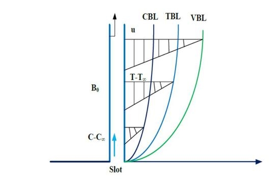
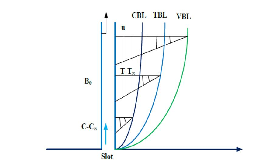
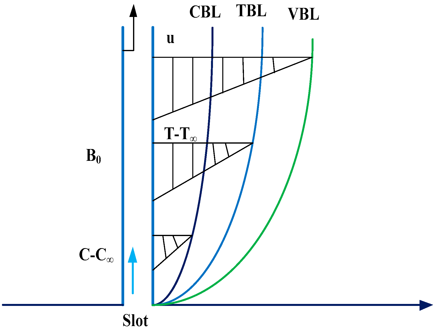
2. Formulation of the Problem
3. Physical Quantities of Interest
4. Solution by HAM
5. Discussion
5.1. Graphical Discussion
5.2. Discussion of Tables
6. Conclusions
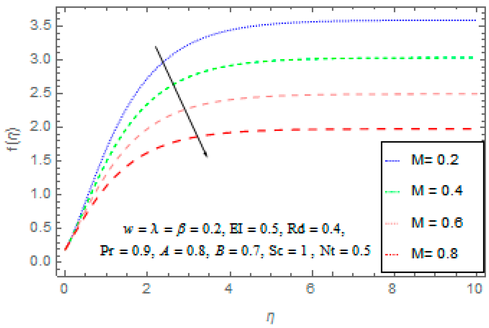
- The magnetic parameter has the reverse effect on velocity, which means that increasing the magnetic field value results in a decrease of the velocity of the nanofluid. This is due to the Lorentz forces, which are against the flow of the fluid.
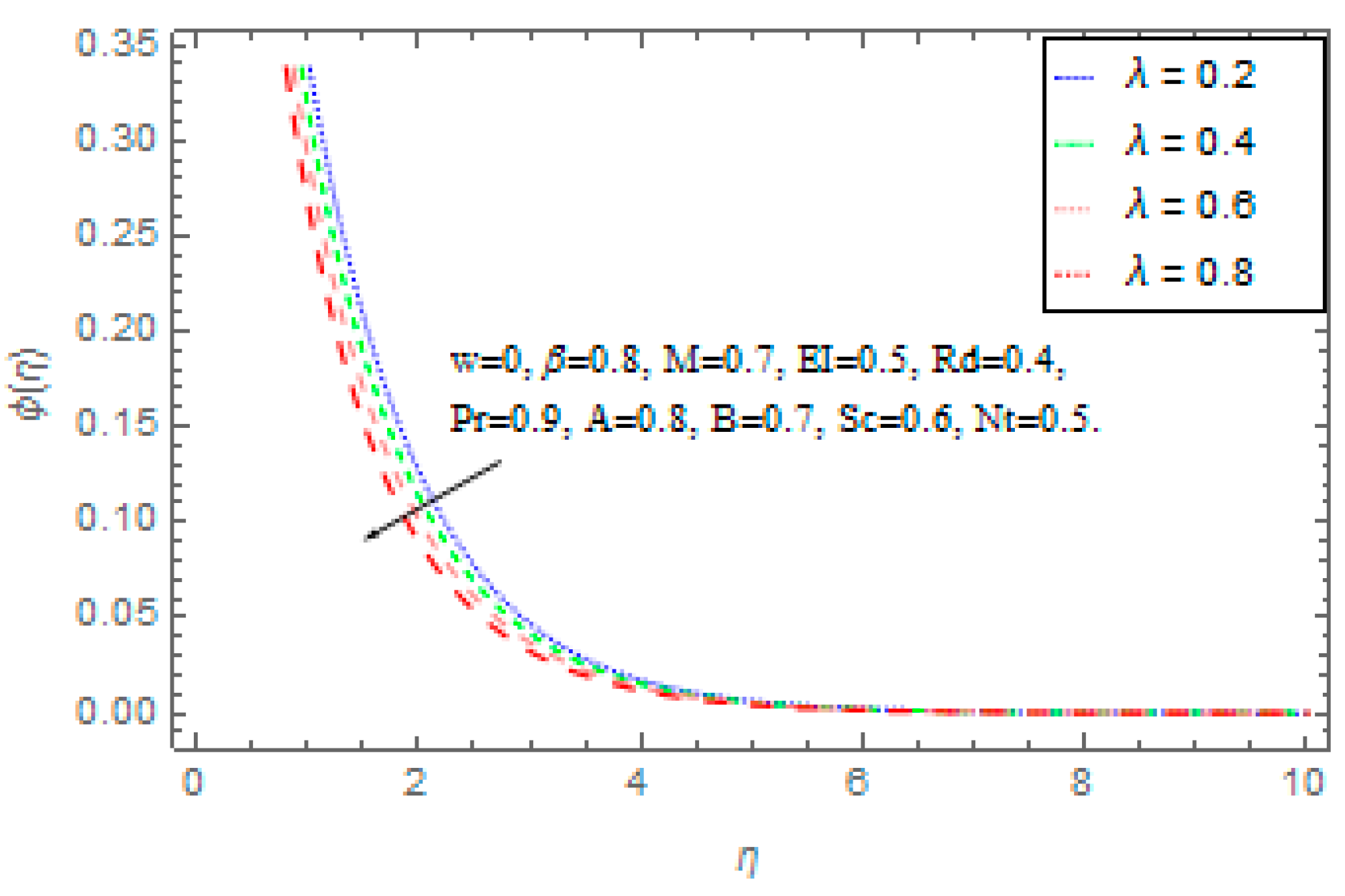
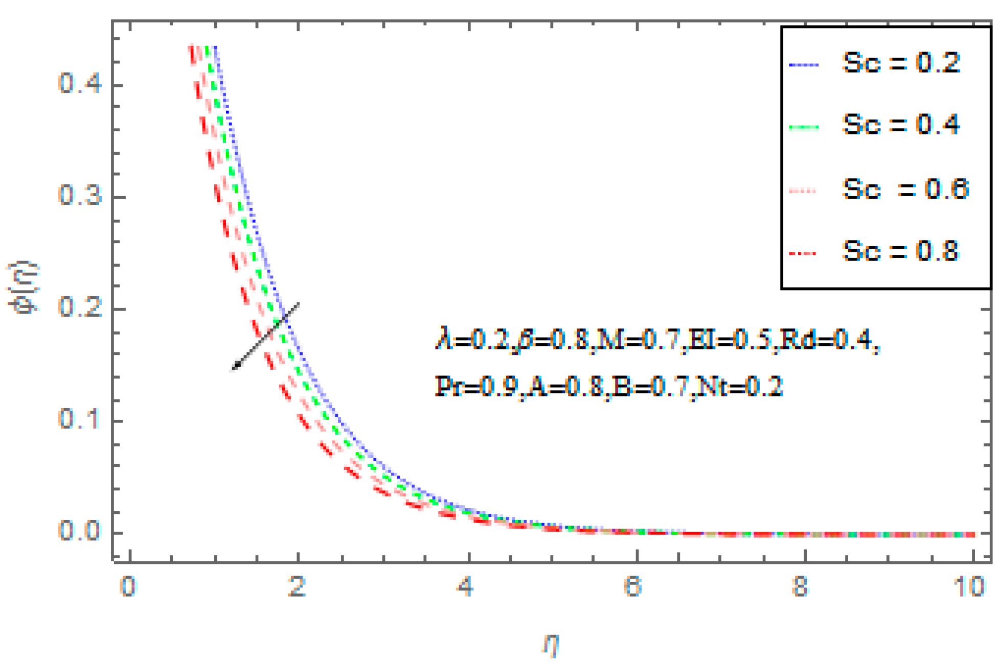
- Increasing Schmidt number decreases the concentration profile , which is consistent with previous results.
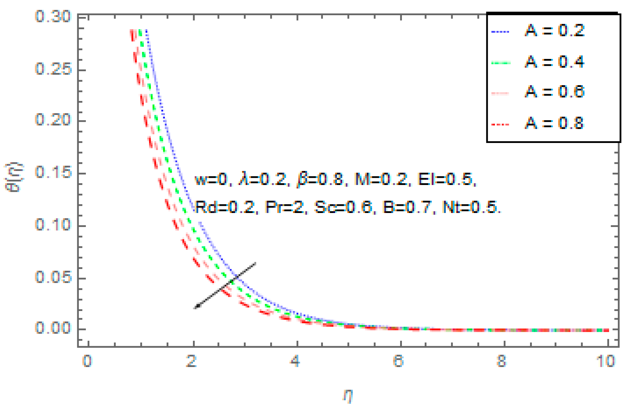
- The unsteady parameter shows decreasing behavior in velocity profile, concentration profile and temperature profile of the fluid.
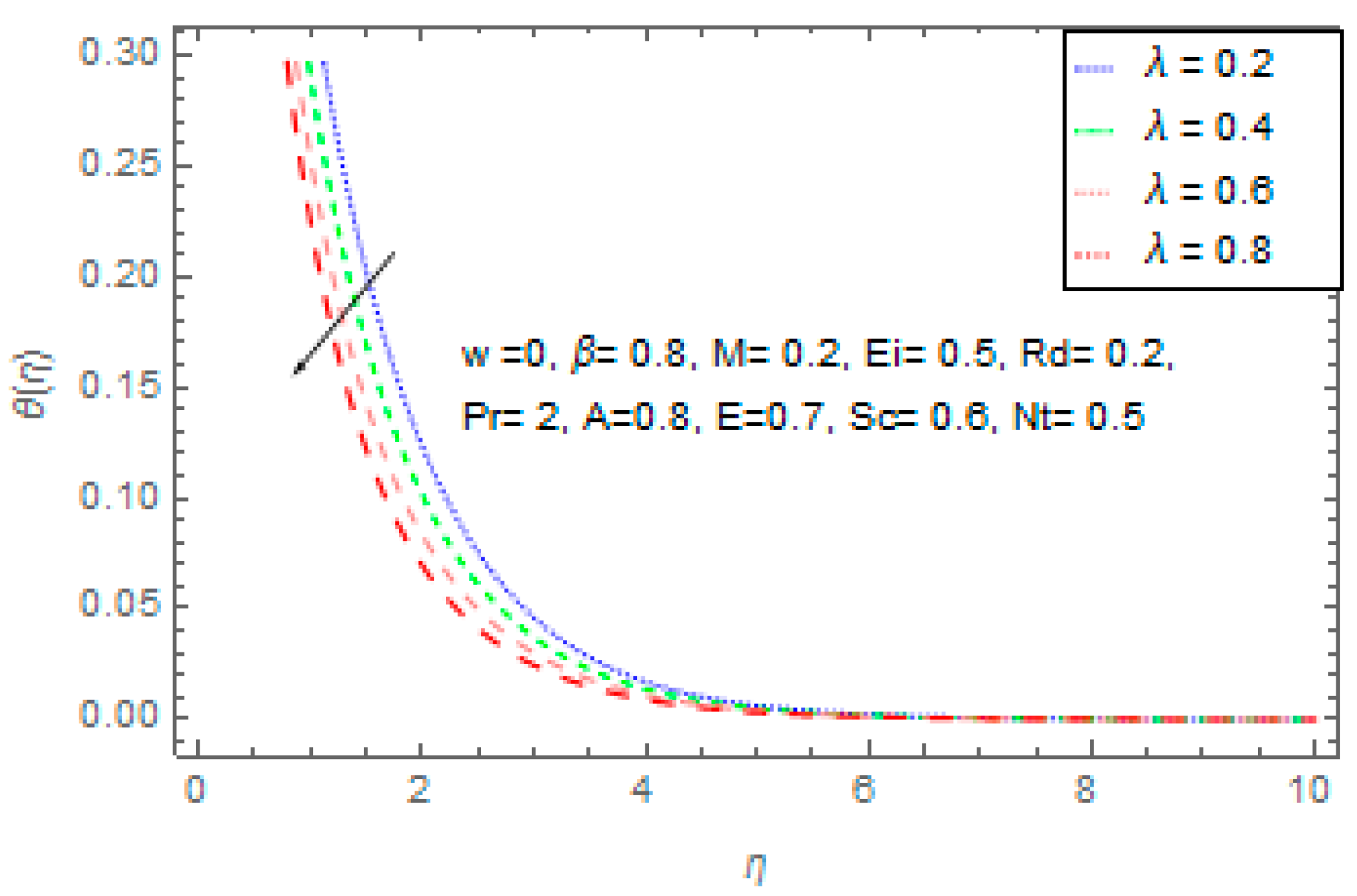
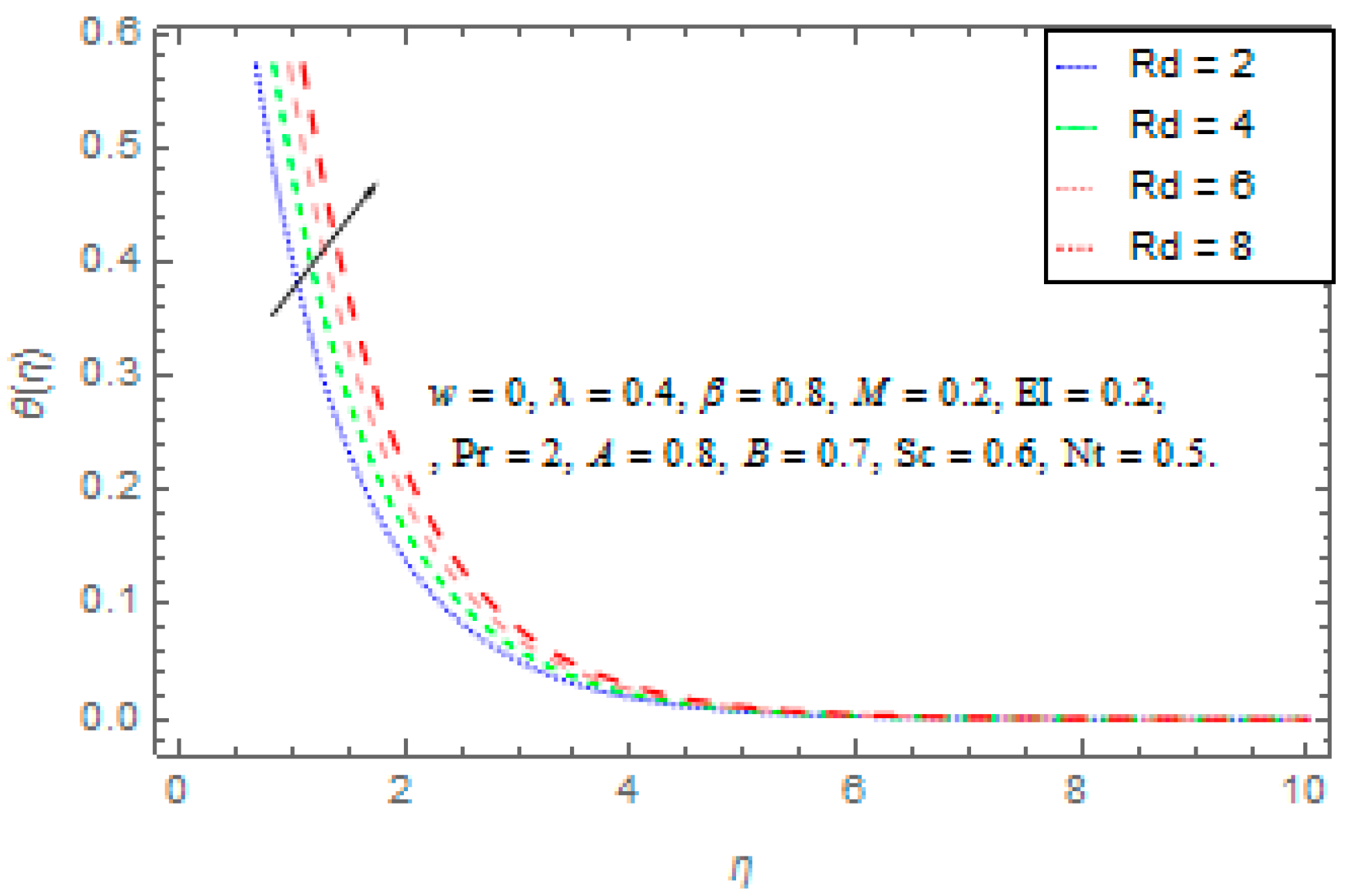
- The effect of radiation on temperature matches common observations. It increases the temperature of the fluid. It is also observed that high radiations cause a high temperature.
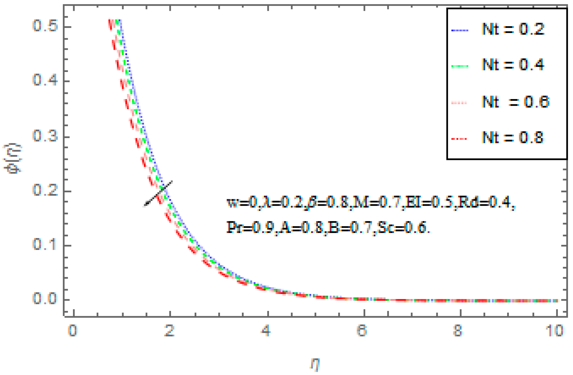
- Increasing the value of the thermophoretic parameter decreases the concentration of the nanofluid.
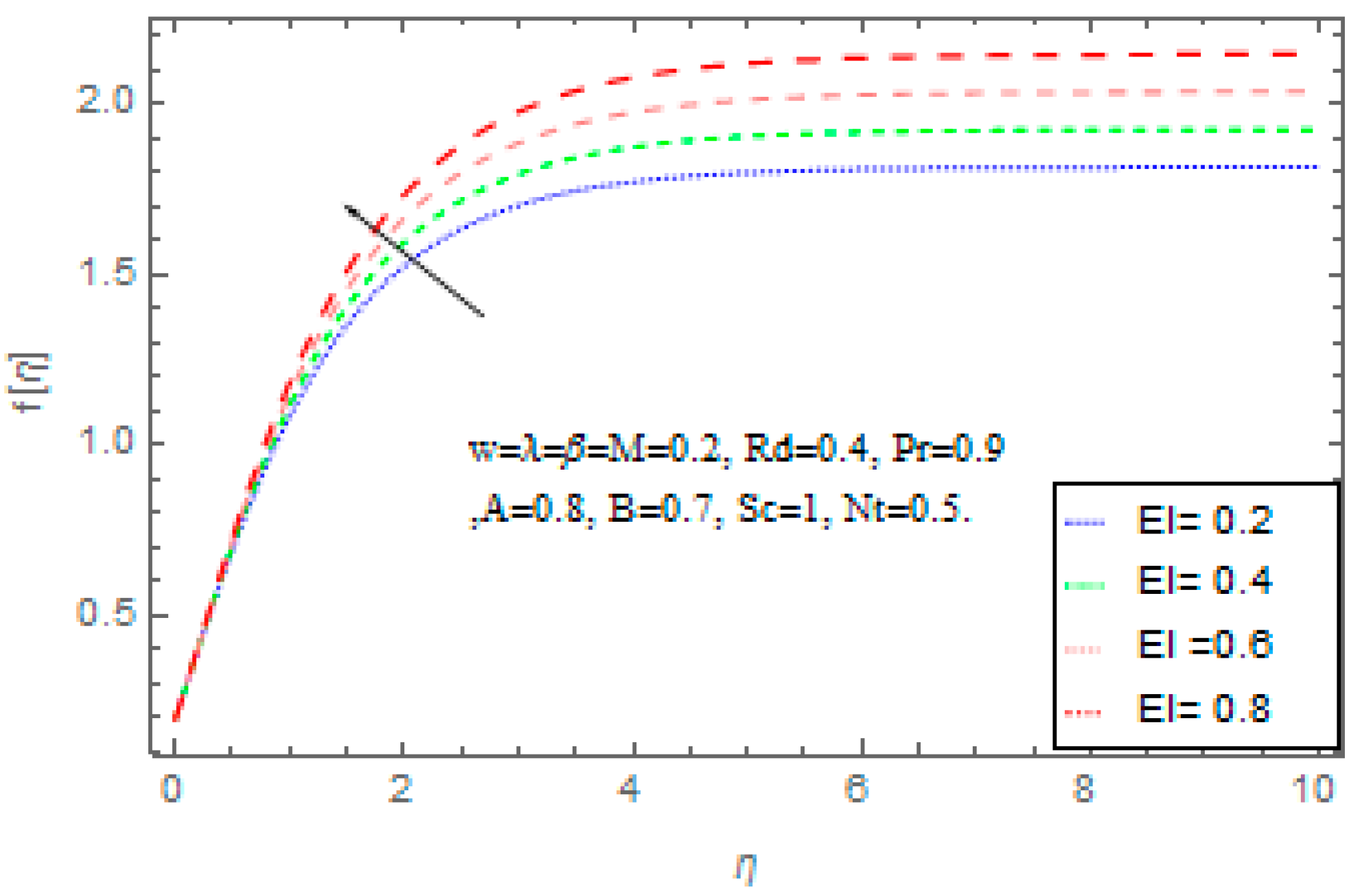
- The velocity of the nanofluid increases with increasing value of the electric field, but the combined effect of the electric and magnetic field produces Lorentz forces, which result in a decrease of the velocity of the fluid.
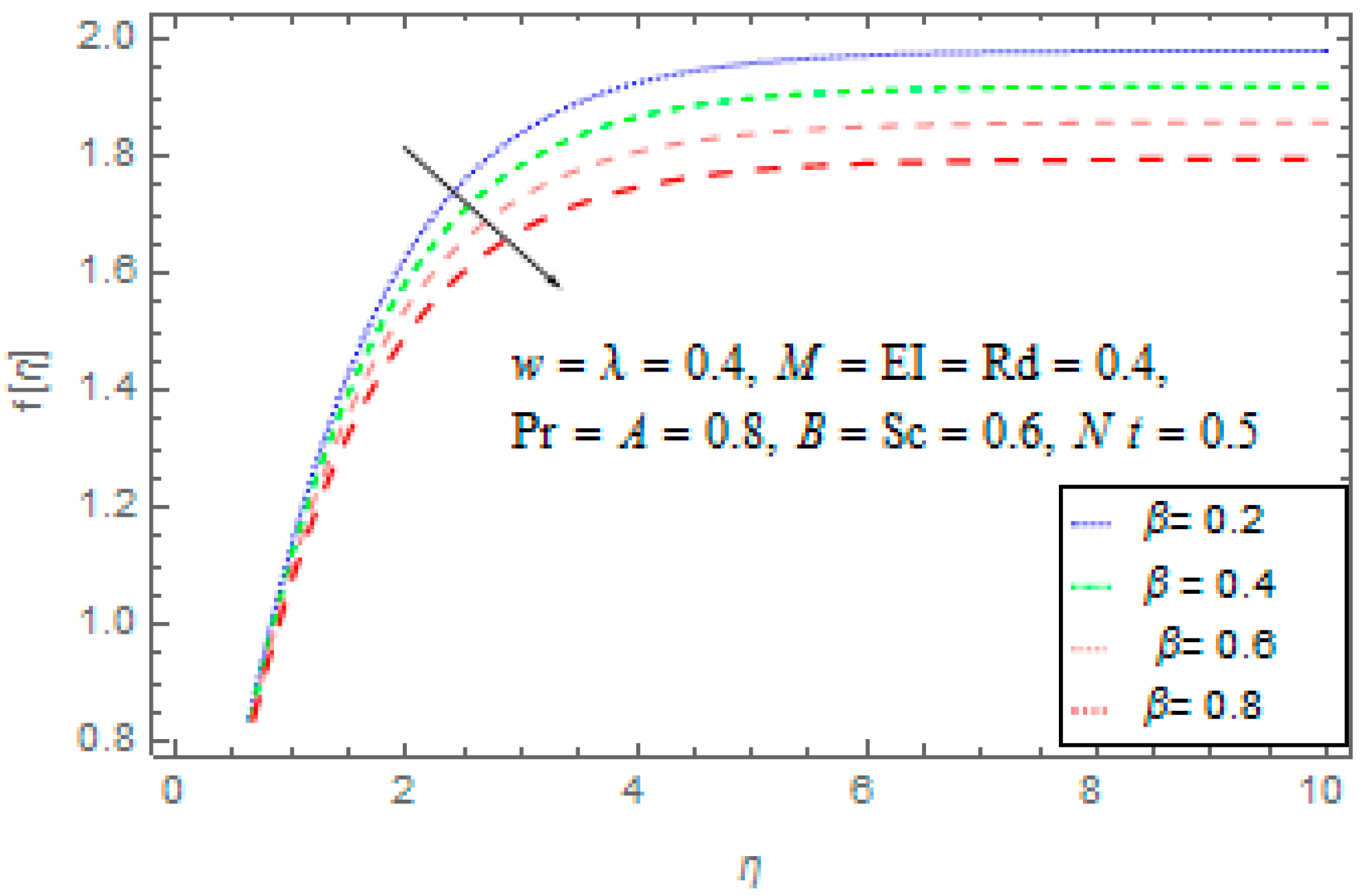
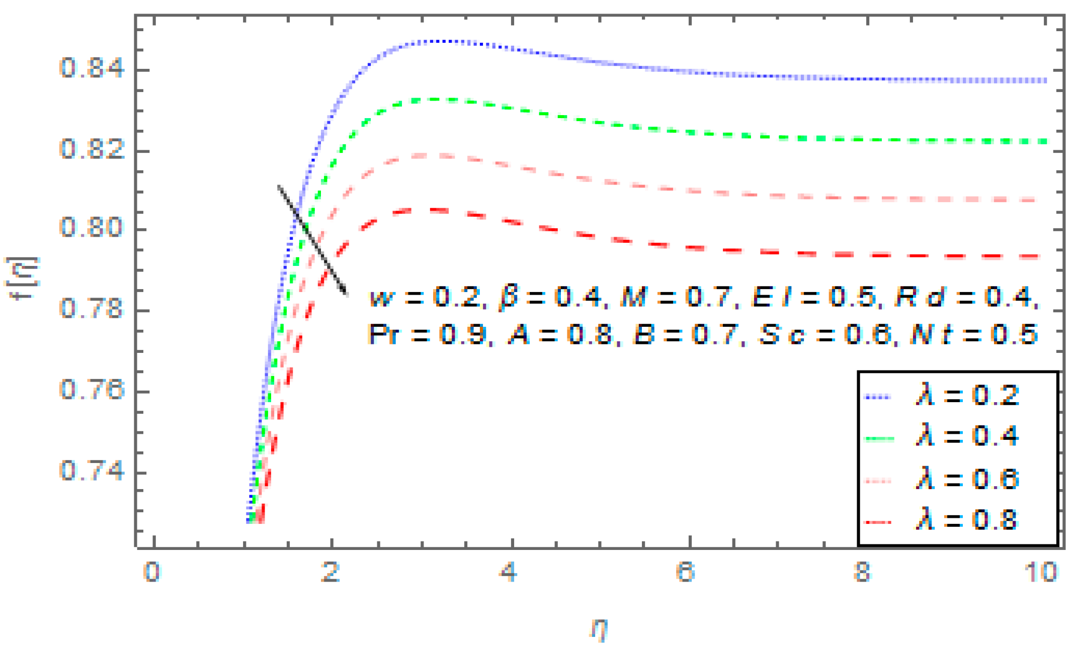
- It is noted that increasing the Deborah number decreases the velocity of the Nanofluid.
Author Contributions
Conflicts of Interest
References
- Alfven, H. Existence of electromagnetic-hydrodynamic waves. Nature 1942, 150, 405–406. [Google Scholar] [CrossRef]
- Mahanthesh, B.; Gireesha, B.J.; Reddy, G.R.S. Unsteady three-dimensional MHD flow of a nano Eyring-Powell fluid past a convectively heated stretching sheet in the presence of thermal radiation, viscous dissipation and Joule heating. J. Assoc. Arab Univ. Basic Appl. Sci. 2017, 23, 75–84. [Google Scholar] [CrossRef]
- Reddy, P.S.; Chamka, A.J. Soret and Dufour Effects on Unsteady MHD Heat and Mass Transfer from a Permeable Stretching Sheet with Thermophoresis and Non-Uniform Heat Generation/Absorption. J. Appl. Fluid Mech. 2016, 9, 2443–2455. [Google Scholar] [CrossRef]
- Choi, S.U.S. Nanofluids from vision to reality through research. J. Heat Transf. 2009, 131, 033106. [Google Scholar] [CrossRef]
- Yu, W.; France, D.M.; Routbort, J.L.; Choi, S.U.S. Review and comparison of nanofluid thermal conductivity and heat transfer enhancements. Heat Transf. Eng. 2008, 29, 432–460. [Google Scholar] [CrossRef]
- Tyler, T.; Shenderova, O.; Cunningham, G.; Walsh, J.; Drobnik, J.; McGuire, G. Thermal transport properties of diamond based nanofluids and nanocomposites. Diam. Relat. Mater. 2006, 15, 2078–2081. [Google Scholar] [CrossRef]
- Das, S.K.; Choi, S.U.S.; Patel, H.E. Heat transfer in nanofluids—A review. Heat Transf. Eng. 2006, 27, 3–19. [Google Scholar] [CrossRef]
- Liu, M.S.; Lin, M.C.-C.; Huang, I.-T.; Wang, C.-C. Enhancement of thermal conductivity with carbon nanotube for nanofluids. Int. Commun. Heat Mass Transf. 2005, 32, 1202–1210. [Google Scholar] [CrossRef]
- Nicolas, G.G.; Antonio, R.; Antonio, G. Electric field induced fluid flow on microelectrodes: the effect of illumination. J. Phys. D Appl. Phys. 2000, 33, L13–L17. [Google Scholar]
- Velkoff, H.R.; Godfrey, R. Low-Velocity Heat Transfer to a Flat Plate in The Presence of a Corona Discharge in Air. J. Heat Transf. 1979, 101, 157–163. [Google Scholar] [CrossRef]
- Yan, Y.Y.; Zhang, H.B.; Hull, J.B. Numerical Modeling of Electrohydrodynamic (EHD) Effect on Natural Convection in an Enclosure. Numer. Heat Transf. Part A Appl. 2004, 46, 453–471. [Google Scholar] [CrossRef]
- Hsu, J.P.; Kao, C.Y.; Tseng, S.; Chen, C.J. Electrokinetic transport in unsteady flow through peristaltic microchannel. J. Colloid Interface Sci. 2002, 248, 176–184. [Google Scholar] [CrossRef] [PubMed]
- Monajjemi, R.E.; Nasr, E.M. Influence of the uniform electric field on viscosity of magnetic nanofluid. J. Appl. Phys. 2012, 112, 094903. [Google Scholar] [CrossRef]
- Plumb, O.A.; Huenfeld, J.S.; Eschbach, E.J. The effect of cross flow and radiation on natural convection from vertical heated surfaces in saturated porous media. In Proceedings of the AIAA 16th Thermophysics Conference, Palo Alto, CA, USA, 23–25 June 1981. [Google Scholar]
- Grubka, L.G.; Bobba, K.M. Heat transfer characteristics of a continuous stretching surface with variable temperature. J. Heat Transf. 2015, 107, 248–250. [Google Scholar] [CrossRef]
- Watson, G.H.; Lee, A.L. Thermal radiation model for solid rocket booster plumes. J. Spacecr. Rockets 1977, 14, 641–647. [Google Scholar] [CrossRef]
- Rajesh, V.; Anwar, B.; Mallesh, M.P. Transint nanofluid flow and heat transfer from a moving vertical cylinder in the presence of thermal radiation. J. Nanomater. Nanoeng. Nanosyst. 2016, 230, 3–10. [Google Scholar]
- Yang, G.; Ebadian, M.A. Radiation convection in a thermally developing duct flow of noncircular cross section. J. Thermophys. Heat Transf. 1999, 5, 224–231. [Google Scholar] [CrossRef]
- Nansour, M.A.; El Shear, N.A. Radiative effects on magnetohydrodynamic Natural Convection flows saturated in porous media. J. Magn. Magn. Mater. 2001, 237, 327–341. [Google Scholar] [CrossRef]
- Sheikholeslamia, M.; Ganji, D.D.; Javed, Y.M.; Ellahi, R. Effect of thermal radiation on magnetohydrodynamics nanofluid flow and heat transfer by means of two phase model. J. Magn. Magn. Mater. 2015, 374, 36–43. [Google Scholar] [CrossRef]
- Sheikholeslamia, M.; Jalili, P. Magnetic field effect on nanofluid flow between two circular cylinders using AGM. Alex. Eng. J. 2017. [Google Scholar] [CrossRef]
- Khanafer, K.; Vafai, K.; Lightstone, M. Buoyancy-driven heat transfer enhancement utilizing nanofluids. Int. J. Heat Mass Transf. 2003, 46, 3639–3653. [Google Scholar] [CrossRef]
- Sheikholeslami, M.; Gorj, B.M.; Ganji, D.D.; Soheil, S. Natural convection heat transfer in a nanofluidfilled inclined L-shaped enclosure. IJST Trans. Mech. Eng. 2014, 38, 217–226. [Google Scholar]
- Safia, A.; Nadeem, S. Consequence of nanofluid on peristaltic transport of a hyperbolic tangentfluid model in the occurrence of apt (tending) magnetic field. J. Magn. Magn. Mater. 2014, 358–359, 183–191. [Google Scholar]
- Safia, A.; Nadeem, S.; Anwar, H. Effects of heat and mass transfer on peristaltic flow of a Bingham fluid in the presence of inclined magnetic field and channel with different wave forms. J. Magn. Magn. Mater. 2014, 362, 184–192. [Google Scholar]
- Sheikholeslami, M.; Gorji, B.M.; Ganji, D.D. Natural convection in a nanofluidfilled concentric annulus between an outer square cylinder and an inner elliptic cylinder. Sci. Iran. 2013, 20, 1241–1253. [Google Scholar]
- Safia, A.; Nadeem, S.; Hanif, M. Numerical and analytical treatment on peristalticflow of Williamsonfluid in the occurrence of induced magnetic field. J. Magn. Magn. Mater. 2013, 346, 142–151. [Google Scholar]
- Fetecau, C.; Corina, F. Starting solutions for the motion of a second grade fluid due to longitudinal and torsional oscillations of a circular cylinder. Int. J. Eng. Sci. 2006, 44, 788–796. [Google Scholar] [CrossRef]
- Frank, M.; Drikakis, D. Solid-like heat transfer in confined liquids. Microfluid. Nanofluid. 2017, 21, 148. [Google Scholar] [CrossRef]
- Frank, M.; Drikakis, D.; Asproulis, N. Thermal Conductivity of Nanofluid in Nanochannels. Microfluid. Nanofluid. 2015, 19, 1011–1017. [Google Scholar] [CrossRef] [Green Version]
- Papanikolaou, M.; Frank, M.; Drikakis, D. Nanoflow over a fractal surface. Phys. Fluids 2016, 28, 082001. [Google Scholar] [CrossRef]
- Sakiadis, B.C. Boundary layer behavior on continuous solid surfaces. AIChE J. 1961, 7, 26–28. [Google Scholar] [CrossRef]
- Crane, L.J. Flow past a stretching sheet. Z. Angew. Math. Phys. 1970, 21, 645–647. [Google Scholar] [CrossRef]
- Gupta, P.S.; Gupta, A.S. Heat and mass transfer on a stretching sheet with suction or blowing. Can. J. Chem. Eng. 1977, 55, 744–746. [Google Scholar] [CrossRef]
- Takahashi, N.; Koseki, H.; Hirano, T. Temporal and spatial characteristics of radiation from large pool fires Bull. Jpn. Assoc. Fire Sci. Eng. 1999, 49, 27–33. [Google Scholar]
- Wang, C.Y. Liquid film on an unsteady stretching surface. Q. Appl. Math. 1990, 48, 601–610. [Google Scholar] [CrossRef]
- Elbashbeshy, E.M.A.; Bazid, M.A.A. Heat transfer over an unsteady stretching surface. Heat Mass Transf. 2004, 41, 1–4. [Google Scholar] [CrossRef]
- Chamkha, A.J.; Ahmed, S.E. Similarity Solution for Unsteady MHD Flow Near a Stagnation Point of a Three Dimensional Porous Body with Heat and Mass Transfer, Heat Generation/Absorption and Chemical Reaction. J. Appl. Fluid Mech. 2011, 4, 87–94. [Google Scholar]
- Molla, M.M.; Saha, S.C.; Hossain, M.A. Radiation effect on free convection laminar flow along a vertical flat plate with stream wise sinusoidal surface temperature. Math. Comput. Model. 2011, 53, 1310–1319. [Google Scholar] [CrossRef] [Green Version]
- Liao, S.J. On the Analytic Solution of Magnetohydrodynamic Flows of Non-Newtonian Fluids over a Stretching Sheet. J. Fluid Mech. 2003, 488, 189–212. [Google Scholar] [CrossRef]
- Liao, S.J. An Analytic Solution of Unsteady Boundary Layer Flows Caused by Impulsively Stretching Plate. Commun. Nonlinear Sci. Numer. Simul. 2006, 11, 326–339. [Google Scholar] [CrossRef]
- Liao, S.J. On Homotopy Analysis Method for Nonlinear Problems. Appl. Math. Comput. 2004, 147, 499–513. [Google Scholar] [CrossRef]
- Asproulis, N.; Kalweit, M.; Drikakis, D. A Hybrid Molecular Continuum Method using Point Wise Coupling. Adv. Eng. Softw. 2012, 46, 85–92. [Google Scholar] [CrossRef]
- Kalweit, M.; Drikakis, D. Coupling strategies for hybrid molecular-continuum simulationmethods. J. Mech. Eng. Sci. 2008, 222, 797–806. [Google Scholar] [CrossRef]
- Kalweit, M. Multiscale Methods for Micro/Nano Flows and Materials. J. Comput. Theor. Nanosci. 2008, 5, 1923–1938. [Google Scholar] [CrossRef]


Reddy et al. [3] Results | Present Results | ||||
|---|---|---|---|---|---|
| 0.1 | −1.5158744 | −1.74875 | |||
| 0.5 | −1.6666449 | −1.91320 | |||
| 1.0 | −1.8346139 | −1.91302 | |||
| 1.5 | −1.9860796 | −2.30777 | |||
| 0.5 | −1.4519989 | −2.11320 | |||
| 0.1 | −1.5557482 | −1.74875 | |||
| 0.5 | −1.6666449 | −1.77085 | |||
| 1.0 | −1.7845786 | −1.79849 | |||
| 1.5 | −1.3363316 | −1.82613 | |||
| 0.5 | −1.3257839 | −1.77085 | |||
| 0.1 | −1.3704027 | −1.62822 | |||
| 0.5 | −1.4023647 | −1.74875 | |||
| 1.0 | −1.1278748 | −1.89622 | |||
| 1.5 | −1.2578397 | −2.04021 | |||
| 0.5 | −1.6594641 | −1.74875 | |||
| 0.1 | −1.7868723 | −1.15896 | |||
| 0.5 | −1.2867381 | −1.62822 | |||
| 1.0 | −1.3188963 | −2.26780 | |||
| 1.5 | −1.3748052 | −2.98208 |
Reddy et al. [3] Results | Presents Results | ||||
|---|---|---|---|---|---|
| 0.1 | 1.0954583 | 0.418189 | |||
| 0.5 | 1.0769383 | 0.365972 | |||
| 1.0 | 1.0581713 | 0.325005 | |||
| 1.5 | 1.0427808 | 0.303409 | |||
| 0.5 | 0.9558400 | 0.365972 | |||
| 0.1 | 1.0142059 | 0.384688 | |||
| 0.5 | 1.0769383 | 0.429300 | |||
| 1.0 | 1.1440810 | 0.484446 | |||
| 1.5 | 1.0638213 | 0.538907 | |||
| 0.5 | 0.8488358 | 0.429300 | |||
| 0.1 | 0.7413729 | 0.712750 | |||
| 0.5 | 0.5802159 | 0.619018 | |||
| 1.0 | 0.9273635 | 0.501853 | |||
| 1.5 | 0.8488358 | 0.384688 | |||
| 0.5 | 0.7619111 | 0.619018 | |||
| 0.1 | 0.6631123 | 0.810743 | |||
| 0.5 | 1.0967356 | 0.712750 | |||
| 1.0 | 0.9541261 | 0.587160 | |||
| 1.5 | 0.7670185 | 0.458056 |
Reddy et al. [3] Results | Present Results | |||
|---|---|---|---|---|
| 0.1 | 1.4353078 | 1.955299 | ||
| 0.5 | 1.4044462 | 1.660820 | ||
| 1.0 | 1.3724033 | 1.407640 | ||
| 1.5 | 1.3455601 | 1.643610 | ||
| 0.5 | 1.2787791 | 1.660820 | ||
| 0.1 | 1.3398008 | 0.836947 | ||
| 0.5 | 1.4044462 | 0.955299 | ||
| 1.0 | 1.4731732 | 1.107160 | ||
| 1.5 | 1.0989064 | 1.263380 | ||
| 0.5 | 1.2599294 | 0.955299 | ||
| 0.1 | 1.3403629 | 0.814646 | ||
| 0.5 | 1.4609154 | 0.844357 | ||
| 1.0 | 1.2046987 | 0.781225 | ||
| 1.5 | 1.2599294 | 0.717796 | ||
| 0.5 | 1.3199523 | 0.844357 |
© 2018 by the authors. Licensee MDPI, Basel, Switzerland. This article is an open access article distributed under the terms and conditions of the Creative Commons Attribution (CC BY) license (http://creativecommons.org/licenses/by/4.0/).
Share and Cite
Khan, H.; Haneef, M.; Shah, Z.; Islam, S.; Khan, W.; Muhammad, S. The Combined Magneto Hydrodynamic and Electric Field Effect on an Unsteady Maxwell Nanofluid Flow over a Stretching Surface under the Influence of Variable Heat and Thermal Radiation. Appl. Sci. 2018, 8, 160. https://doi.org/10.3390/app8020160
Khan H, Haneef M, Shah Z, Islam S, Khan W, Muhammad S. The Combined Magneto Hydrodynamic and Electric Field Effect on an Unsteady Maxwell Nanofluid Flow over a Stretching Surface under the Influence of Variable Heat and Thermal Radiation. Applied Sciences. 2018; 8(2):160. https://doi.org/10.3390/app8020160
Chicago/Turabian StyleKhan, Hameed, Muhammad Haneef, Zahir Shah, Saeed Islam, Waris Khan, and Sher Muhammad. 2018. "The Combined Magneto Hydrodynamic and Electric Field Effect on an Unsteady Maxwell Nanofluid Flow over a Stretching Surface under the Influence of Variable Heat and Thermal Radiation" Applied Sciences 8, no. 2: 160. https://doi.org/10.3390/app8020160