Production and Maintenance Planning for a Deteriorating System with Operation-Dependent Defectives

Abstract

This paper provides new insights to the area of sustainable manufacturing systems at analyzing the novel paradigm of integrated production logistics, quality, and maintenance design. For this purpose, we investigate the optimal production and repair/major maintenance switching strategy of an unreliable deteriorating manufacturing system. The effects of the deterioration process are mainly observed on the failure intensity and on the quality of the parts produced, where the rate of defectives depends on the production rate. When unplanned failures occur, either a minimal repair or a major maintenance could be conducted. The integration of availability and quality deterioration led us to propose a new stochastic dynamic programming model where optimality conditions are derived through the Hamilton-Jacobi-Bellman equations. The model defined the joint production and repair/major maintenance switching strategies minimizing the total cost over an infinite planning horizon. In the results, the influence of the deterioration process were evident in both the production and maintenances control parameters. A numerical example and an extensive sensitivity analysis were conducted to illustrate the usefulness of the results. Finally, the proposed control policy was compared with alternative strategies based on common assumptions of the literature in order to illustrate its efficiency.

1. Introduction

Manufacturing systems rarely perform exactly as expected and predicted, since they may experience disorders from many unexpected events, such as equipment break-downs, delays, defectives, deterioration, etc., as reported in Liberopoulos et al. [1]. In this context, quality, production planning and maintenance define the fundamental functions to achieve success in the manufacturing industry, implying resource efficiency along the product, process, and production system life-cycle. Therefore, integrated operations management approaches are needed to have a global vision of the company by taking into account the interactions between the different key functions. This paper aims to develop an effective method for decision making on industrial strategies under integrated approach of the production control, quality, and maintenance planning.

There is a broad variety of practical problems dealing with the association between production and quality. It is clear that equipment availability, product quality, and productivity are strongly interrelated. However, these fields have been traditionally treated by manufacturers and researchers almost in isolation. Some authors have proposed frameworks for the joint production-quality relationship as in Colledani and Tolio [2], who presented an analytical method for evaluating the performance of production systems, jointly considering quality and production performance indices. Yedes et al. [3] studied a production unit that randomly shifts from an in-control to an out-of control state, where at the end of the production cycle, maintenance activities are performed depending on the state of the unit. The simulation work proposed by Rivera-Gómez et al. [4] addressed the problem of an unreliable manufacturing system that produces conforming and non-conforming parts, where due to the wear of the system, the authors considered the use of external production to supplement the limited production capacity. An algorithm integrating production and quality issues were presented by Mhada et al. [5], where they determined the buffer sizing and inspection positioning problem of large production lines, identifying promising locations for the inspection stations. Recently, Bouslah et al. [6] investigated the joint design and optimization of a continuous sampling plan, make-to-stock production and maintenance. They defined the number of successive items clear of defects required to discontinue rigorous inspection, the fraction of product sampling, the maintenance period and the amount of inventory needed as protections against disruptions. According to these studies, the relation between production and quality exists in several ways. Nevertheless, the model developed in our paper is different, because we take into account the fact that production at high rates accelerates the machine degradation and thus increases the total cost of repairs, defectives, production, etc. Therefore, the decisions involved in our formulation seek how to balance production, quality, and maintenances activities for efficient operations management.

The issues related to the maintenance of manufacturing systems are relevant to our research because in modern production systems their components are usually unreliable and so maintenance decisions should be integrated in the decision-making to properly estimate their global effect, as in the work of Mifdal et al. [7]. Who developed a method to find the optimal production rate for a manufacturing system, which produces several products in order to satisfy random demands; also, they established an economical scheduling for preventive maintenance. The study of Khatab et al. [8] addressed the problem of a production system that is continuously monitored and subject to stochastic degradation. To assess such degradation, the system undergoes preventive maintenance whenever its reliability reaches an appropriate value. Hajej et al. [9] study a manufacturing system composed by a failure prone-machine, a manufacturing store, and a purchase warehouse with service level, where a preventive maintenance plan is provided in order to decrease the failure rate. In the study of Askri et al. [10], the authors dealt with a preventive maintenance strategy and the determination of an economical production plan. Their model defines the optimal maintenance interval at which machines are maintained simultaneously. A common feature of the above papers is that they have mainly studied the joint production scheduling and maintenance planning, which has received much attention in the literature, but this does not necessarily lead to an optimal solution. Since they have disregarded the importance of quality aspects in their results. Hence, taking into account the interrelations between production, quality, and maintenance, traditionally approaches may be modified.

In the context of deteriorating systems, machine failure is probably one of the most frequently observed disruption that does deteriorate the system performance. A considerable amount of research has been spurred to address time-dependent failures. However, in most manufacturing systems is often more realistic to assume that machine reliability does depend on the degree of utilization of the machine. Thus, operation-dependent failures are common in such systems, and this assumption renders the problem much more involved, as indicated by Martinelli et al. [11], who provided the structure of a policy minimizing the long-term average backlog and inventory cost for an unreliable machine, where the failure rate is a piecewise constant function of the production rate. In the same vein, Dahane et al. [12] dealt with the problem of dependence between production and failure rates in the context of single randomly failing and repairable manufacturing system producing two products. Haoues et al. [13] were interested in the study of a production unit that aims to satisfy the deterministic market demands for multiple products. They considered that the production cost depends on the using rate of the machine, and that such machine deteriorates with increased use. Other researchers have treated the problem of production-dependent failure rates, for example Kouedeau et al. [14] analyzed a manufacturing system comprising parallel machines with failure rate depending on their productivity. They determined the productivity of the main and the supporting machine. From the discussed papers, it is evident that models considering operation-dependent failures, are rarely studied in the literature, and their focus have been mainly on the dependence between production and failure rate. Thus, one drawback of these papers is that the connection between productivity and quality deterioration have not been considered. In contrast, since deterioration is a common industrial phenomenon, our model aims to extend the concept of deterioration to state that indeed production at higher rates accelerates the machine degradation, and their effect not only may increase the failure rate but also may decline product quality.

Our research aims to generalize previous assumptions and extent several conjectures reported in the literature. In particular, we extend the work of Martinelli et al. [11], Hajej et al. [9], and Kouedeau et al. [14] in several directions: (i) at presenting an integrated production-maintenance-quality approach which serves to analyze the interactions between these three key functions; (ii) at studying the impact of a double deterioration process with continuous deterioration of part quality and reliability; (iii) at considering the dependence between productivity and product quality, leading to define operation-dependent defectives. We note that these set of characteristics have not been treated simultaneously in the literature yet. We developed a stochastic optimal control model to determine the structure of the control policy. Moreover, the obtained results are examined thorough an extensive sensitivity analysis.

The remainder of the paper is organized as follows: in the next section, the industrial motivation of the paper is presented. Section 3 describes the notation and formulation of the proposed model. In Section 4, the optimization method that is applied is detailed. The obtained joint control policy is presented in Section 5. A sensitivity analysis is carried out in Section 6. A comparative study is conducted in Section 7. Some managerial implications are discussed in Section 8. Finally, conclusions and future scope of research are provided in Section 9.

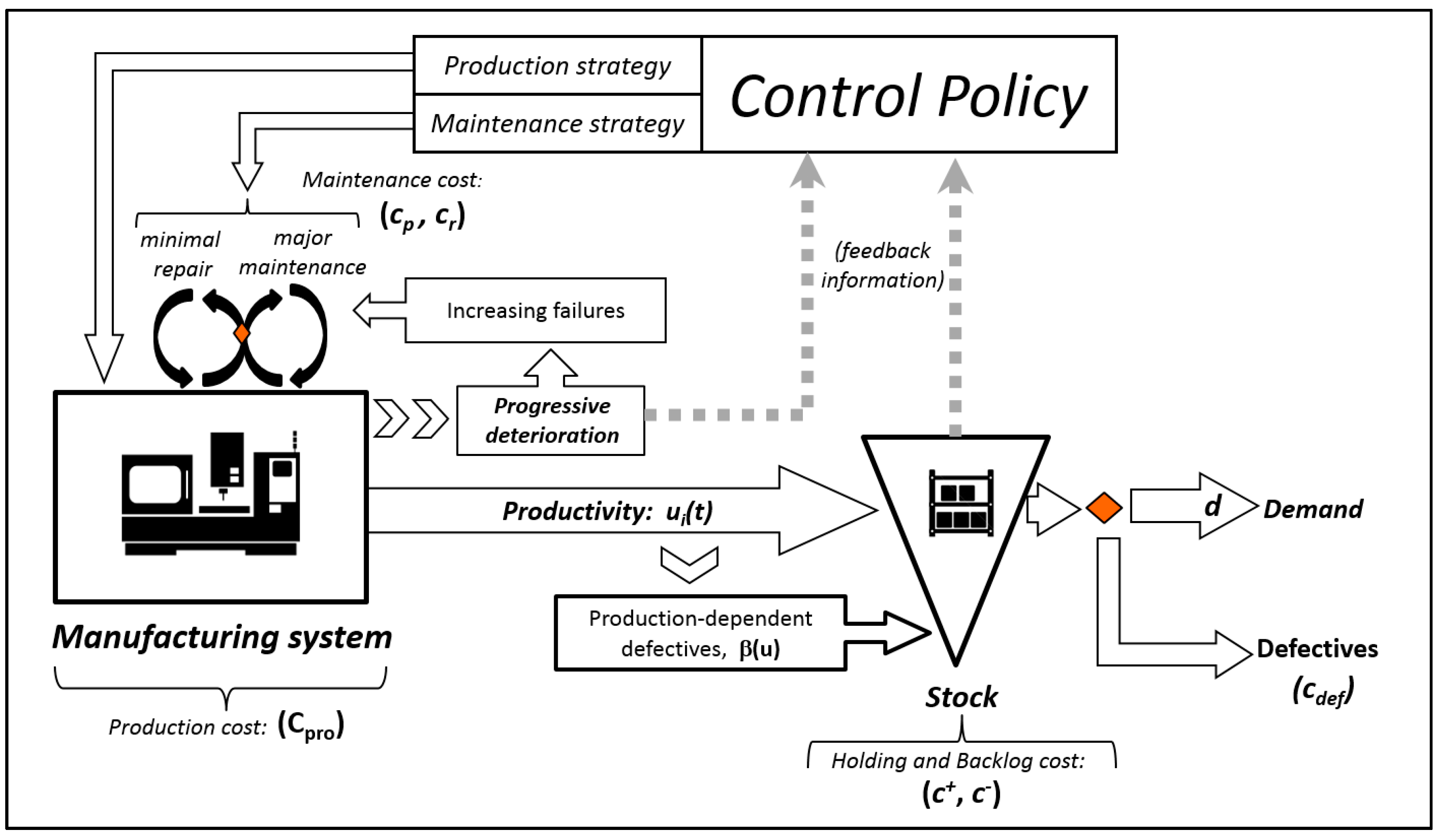
2. Industrial Motivation

In a manufacturing environment, it exits a vast number of potential disruptions that negatively affect the system’s performance such as failures, wear, shortages, defectives, etc. Among these disruptions, machine failures are the most frequent problem observed in manufacturing systems. Furthermore, more realistic models are conceived at considering that machine reliability does depend on the degree of utilization of the machine leading to define operation-dependent failures, as indicated by Dong-Ping [15]. Although, such type of failures is common in production systems, they are rarely considered by researchers and practitioners. Additionally, during the last years the focus has been on the dependence between productivity and the failure rate, and just some works have studied the connection between operation-dependent failures and deterioration, as in Kouedeau et al. [14]. Nevertheless, in modern production systems, deterioration is a common industrial phenomenon. Hence, this observation raises the question of whether at considering a deterioration process, the production at higher rates may accelerate the machine degradation, indicating a dependence between deterioration and several system’s performance indices such as product quality, reliability, safety, etc. Conversely, producing at low rates may contribute to an increase of shortages and incur economic losses. Thus, given the dependency of the involved cost and productivity, a trade-off is implied, and it would be advantageous to reduce the production rate from its maximum value to a more profitable level to reduce for instances the increase of defective units and failures.

The model presented in this paper has many applications especially in industries characterized by deterioration, where the production system is subject to random failures and repairs, defective quality is present and their production rates can be controlled. In particular, in situations where the production system deteriorates over time such as the automotive sector, pharmaceutical, semiconductor industries, etc.

3. Notation and Problem Statement

In this section, we define the notation used in the model formulation, also we define the manufacturing system under analysis.

3.1. Notations

The proposed model is based on the following notations:

$x(t)$	Inventory level at time t
$a(t)$	Age of the machine at time t
$u(t)$	Production rate at time t
$\xi (t)$	Stochastic process
$u_{max}$	Maximal production rate
$u_i$	Productivities of the machine
$w(t)$	Control variable for the repair/major maintenance policy at time t
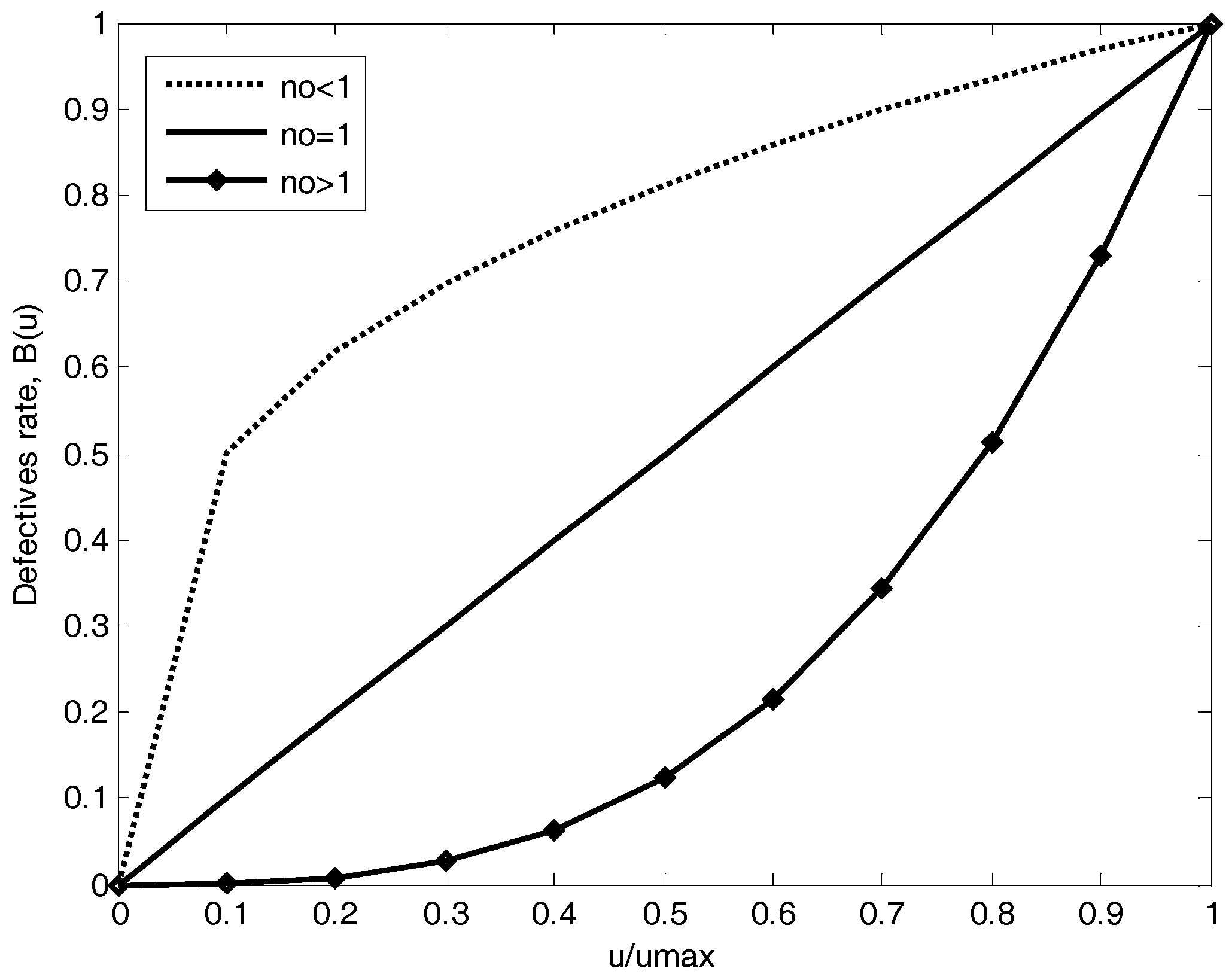
$\beta (·)$	Rate of defectives
$d$	Constant demand rate of products
$\Omega$	Set of states of the machine
$\rho$	Discount rate
${\pi }_i$	Limiting probability at mode i
${\lambda }_{\alpha \alpha \prime }$(·)	Transition rate from mode α to mode α′
$g(·)$	Instantaneous cost function
$J(·)$	Expected discounted cost function
$v(·)$	Value function
$\tau$	Jump time of ξ(t)
$c^{+}$	Inventory holding cost/units/time units
$c^{-}$	Backlog cost/units/time units
$c_r$	Repair cost
$c_m$	Major maintenance cost
$c_d$	Cost of defectives
$c_{pro}$	Cost of production per unit of produced parts
$\theta$	Adjustment parameter for the rate of defectives

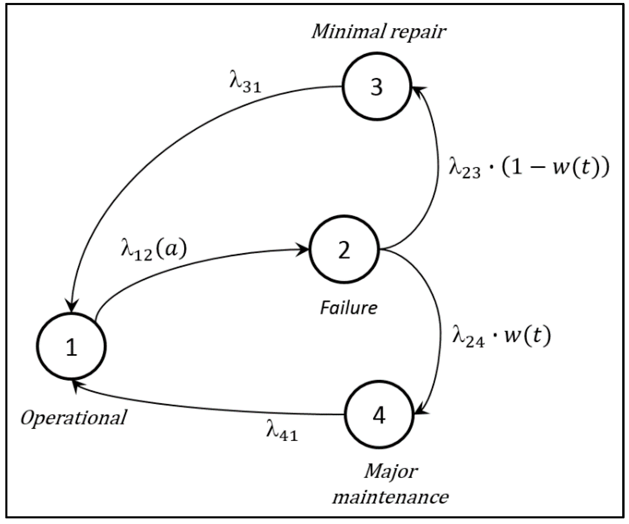
3.2. Problem Description

The manufacturing system under study consists of a single machine producing one part type. Nonetheless, the machine is unreliable and is subject to random events such as failures and maintenances actions of random duration. The machine can produce at diverse capacities to satisfy a constant product demand. Additionally, our considered systems has two principal features, where its failure rate increases in function of its level of deterioration, and the quality of the items produced is not perfect, there is a rate of non-conforming units. Such rate of defectives depends on the productivity of the system, thus defining a productivity-dependent defectives rate. Therefore, the system deteriorates with age and its production pace. These assumptions are common in production management. The stock is a mixture of flawless and defective product and serves as protections against shortages. To cope with the effects of the deterioration process, when the machine is at failure a fundamental problem of the decision-maker is to decide between the conduction of:

• A minimal and inexpensive repair that serves to operate the machine for a while, but with the disadvantage that it does not restore the effect of deterioration, it leaves the machine in as-bad-as-old conditions, ABAO.
• An expensive major maintenance, which mitigates completely the effects of deterioration, leaving the machine in as-good-as-new-conditions, AGAN.

We intend to determine an optimal control policy that defines the appropriate production pace and the repair/major maintenance switching strategy that minimizes the average total cost comprising the inventory, backlog, defectives, production, and maintenance cost. Figure 1, illustrates the block diagram of the manufacturing system under analysis.

3.3. Problem Formulation

We start by conjecturing that the manufacturing system analyzed in this paper consists of an unreliable machine subject to a double deterioration process producing a single part type. The machine mode is described by the stochastic process $\xi (t)\in \Omega =\{1,2,3,4\}$. More precisely, the machine is available when it is operational $(\xi (t)=1),$ an unavailable when it is at failure $(\xi (t)=2)$. Once at failure, the decision-maker must decide between two types of maintenance actions available. When $(\xi (t)=3)$, a minimal repair is conducted where the machine has the same failure rate as before failure, in other words, it restores the system to ABAO conditions. Furthermore, when $(\xi (t)=4)$ a major maintenance is performed mitigating all the effects of the deterioration process, thus restoring the system to AGAN conditions. The transitions rates of the system ${\lambda }_{\alpha {\alpha }^{\prime }}$, from state α to ${\alpha }^{\prime }$, are statistically described by the state probabilities:

$$\begin{gathered} P[\xi (t+\delta t)=\alpha |\xi (t)={\alpha }^{\prime },x(t)=x,a(t)=a] \\ =\{\begin{array}{cc}{\lambda }_{\alpha {\alpha }^{\prime }}(·)\delta t+o(x,a,\delta t)& if\alpha \ne \alpha \prime \hfill \\ 1+{\lambda }_{\alpha {\alpha }^{\prime }}(·)\delta t+o(x,\mathrm{a},\delta t)& if\alpha =\alpha \prime \hfill \end{array} \end{gathered}$$

(1)

with

$$\underset{\delta t\to 0}{\lim }\frac{o(\delta t)}{\delta t}=0;{\lambda }_{\alpha \alpha \prime }(·)=-{\displaystyle \sum }_{\alpha \ne {\alpha }^{\prime }}{\lambda }_{\alpha {\alpha }^{\prime }}(·)$$

(2)

$${\lambda }_{\alpha {\alpha }^{\prime }}(·)\ge 0,(\alpha \ne {\alpha }^{\prime }),\forall \alpha ,{\alpha }^{\prime }\in \mathsf{\Omega }.$$

(3)

The stochastic process defines a generator matrix $\mathit{Q}(·)=({\lambda }_{\alpha {\alpha }^{\prime }}(·))$, which is defined as follows:

$$\mathit{Q}(·)=\left[\begin{array}{cccc}{\lambda }_{11}& {\lambda }_{12}(a)& 0& 0\\ 0& {\lambda }_{22}& 0& {\lambda }_{34}\\ {\lambda }_{31}& 0& {\lambda }_{33}& 0\\ {\lambda }_{41}& 0& 0& {\lambda }_{44}\end{array}\right].$$

(4)

The transition diagram of the system is presented in Figure 2.

The transition rate ${\lambda }_{12}(a)$ implies that the failure rate of the machine depends on its age. The rate ${\lambda }_{23}$ defines the transition from the failure mode to the minimal repair mode. The inverse $[{\lambda }_{23}·(1-w(t))]$ represents the expected delay between a call for the technician and his arrival. A similar delay is represented by the reciprocal $[{\lambda }_{24}·w(t)]$ when the machine is send to major maintenance. Transitions ${\lambda }_{31}$ and ${\lambda }_{41}$ implies that the maintenance durations are defined by an exponential random variable with constant mean. Additionally, we define a binary variable $w(t)\in \{0,1\}$ that allows us to properly synchronize the transitions to the maintenance options available, as denoted in the following expression:

$$\omega (t)=\{\begin{array}{l}\begin{array}{cc}0& ifminimalrepairisperformed\end{array}\\ \begin{array}{cc}1& ifmajormaintenanceisconducted\end{array}\end{array}.$$

(5)

One noteworthy feature of the model is the assumption of production-dependent defectives, which implies that when the machine operates at a higher production rate, it is more likely to deteriorate faster, generating more defectives. Hence, to make this more precise, we state that the defectives rate $\beta (·)$ depends on the production rate $u(t)$ according to the following expression:

$$\beta (u(t))=\{\begin{array}{ll}{b}_1& ifu(t)<u_1\\ b_2& ifu(t)\in (u_1,u_2]\\ \dots & \dots \\ b_k& ifu(t)\in (u_{k-1},u_k]\\ \dots & \dots \\ b_n& ifu(t)\in (u_{n-1},u_{max}]\end{array}$$

(6)

with $b_n\ge \dots \ge b_2\ge b_1$, and 0 $\le u_1\le u_2\le \dots \le u_{max}$. Where $b_k$ and $u_k$ are given constants. More precisely, the value of constants $b_k$ of the defectives rate has the general form, (Kouedeu et al. [14]):

$$b_k={\eta }_0{(\frac{u_k}{u_{max}})}^{{\eta }_1}$$

(7)

where ${\eta }_0$ and ${\eta }_1$ are known positive constants and $u_{max}$ is the maximum production rate. Equation (7) serves to define the value of constant $b_k$. Figure 3 presents the trend of the rate of defectives $\beta (·)$ for different values of ${\eta }_0$ and ${\eta }_1$. We can observe in Figure 3, the considerable influence of the productivity of the machine on the rate of defectives.

At considering the presence of defectives, the evolution of the stock level $x(t)$ is defined by the following differential equation:

$$\frac{dx(t)}{dt}=u(t)-d[1+\beta (u(t))],x(0)=x_0.$$

(8)

The constant $x_0$ defines the initial stock level and $d$ denotes the demand rate. Concerning the evolution of the age of the machine $a(t)$, it implies an increasing function of the number of parts produced, and it is defined by the next differential equation:

$$\frac{da(t)}{dt}=ku(t)$$

(9)

$$a(T)=0$$

(10)

with $k$ as a given positive constant and $T$ is the last restart time of the machine. Furthermore, bearing in mind that the deterioration process also has an effect on the reliability of the machine, in particular in its failure rate ${\lambda }_{12}(·)$. Then the lifetime distribution of a new machine follows an increasing function, as in Love et al. [16]:

$${\lambda }_{12}(a(t))={\lambda }_1+{\lambda }_2[1-e^{-r\theta a{(t)}^{{\eta }_2}}]$$

(11)

where the parameter $\theta$ is useful to adjust the trend of the failure rate and $0\le \theta \le 1$, ${\lambda }_1$ is the failure rate in AGAN conditions, ${\lambda }_2$ is the limit considered in the deterioration process for the rate ${\lambda }_{12}(·)$, $r$, and ${\eta }_2$ are non-negative constants. At selecting appropriate values for $r$, Equation (11) can model increasing functions similar to the Weibull distribution. We present in Figure 4, the trend of the failure rate for different values of the adjustment parameter $\theta$.

The decision variables of the model are the production rate $u(t)$, and the maintenance switching strategy $\omega (t)$. Thus, the set of feasible control policies $\mathsf{\Gamma }(\alpha )$, including $(u(t),\omega (t))$ is given by:

$$\Gamma (\alpha )=\{\left(u(t),\omega (t)\right)\in R^2,0\le u(t)\le u_{max},\omega (t)\in \{0,1\}\}.$$

(12)

We are now able to define the cost rate of the model as:

$$\mathrm{g}(\alpha ,x,a)=c^{+}{x}^{+}+c^{-}{x}^{-}+c_d·\mathsf{\beta }(u(t))·d+c_{pro}·u(t)+c_r·Ind\{\xi (t)=3\}+c_m·Ind\{\xi (t)=4\}$$

(13)

with:

$$x^{+}=max(0,x)$$

$$x^{-}=max(-x,0)$$

$$Ind(\xi (t)=\alpha )=\{\begin{array}{cc}\begin{array}{c}1\\ 0\end{array}& \begin{array}{c}\mathrm{if}\xi (t)=\alpha \\ otherwise\end{array}\end{array}$$

where the cost parameters $c^{+}$ and $c^{-}$ are used to penalize inventory and backlog, respectively. The parameter $c_d$ denotes the defective cost originated by the additional handling and inspection, $c_{pro}$ denotes the production cost, $c_r$ is the minimal repair cost and $c_m$ is the major maintenance cost. The objective in our model implies the determination of the optimal control policies that minimizes the integral of the following expected discounted cost:

$$v(\alpha ,x,a)=\underset{\begin{array}{c}(u(t),\omega (t))\in \Gamma (\alpha )\end{array}}{\inf }E\left[\underset{0}{\overset{\infty }{{\displaystyle \int }}}{e}^{-\rho t}g(·)dt|\alpha (0),x(0),a(0)\right]$$

(14)

where $\rho$ denotes a positive discounted rate, and $v(·)$ defines the value function of the model. Based on the optimality principle, and at defining the cost-to-go function as $v(·,t)$, we can break-up the integral of Equation (14) as follows:

$$v(\alpha ,x,a,t)=\underset{\begin{array}{c}u(t),\omega (t)\\ 0\le t\le \infty \end{array}}{\mathit{inf}}E\left[\underset{0}{\overset{t}{{\displaystyle \int }}}{e}^{-\rho t}g(·)dt+\underset{t}{\overset{\infty }{{\displaystyle \int }}}{e}^{-\rho t}g(·)dt|\alpha (0),x(0),a(0)\right].$$

(15)

Upon defining Equation (15), we note that the second integral of its right-hand-side is the value function in the interval $[t,\infty )$. Additionally, at reducing the discount factor $\rho ,$ expanding the first order derivative of $v(·,t),$ eliminating the expectation symbol, among other manipulations, we get $\forall \alpha \in \Omega$:

$$\begin{gathered} \rho v(\alpha ,x,a)=\underset{(u(t),w(t))\in \Gamma (\alpha )}{\mathit{min}}[g(·)+[u(t)-d[1+\beta (u(t))]]\frac{\partial v(\alpha ,x,a)}{\partial x}+[ku(t)]\frac{\partial v(\alpha ,x,a)}{\partial a} \\ +{\displaystyle \sum }_{\alpha \in \Omega }{\lambda }_{\alpha \alpha \prime }(·)v(\alpha ,x,\phi (\xi ,a))(\alpha )] \end{gathered}$$

(16)

with the following reset function:

$$\phi (\xi ,a)=\{\begin{array}{cc}\begin{array}{c}0\\ a({\tau }^{-})\end{array}& \begin{array}{c}if\xi ({\tau }^{+})=1and[\xi ({\tau }^{-})=4andw(t)=1]\\ otherwise\end{array}\end{array}.$$

(17)

Condition (10) implies that a major maintenance restores the cumulative age to a zero value. Then Equation (17) models the benefit of major maintenance. Further, $\frac{\partial }{\partial x}v(·)$ and $\frac{\partial }{\partial a}v(·)$ refer to the partial derivatives of the value function $v(\alpha ,x,a)$. The importance of Expression (16) relies on the fact that it is the fundamental Hamilton-Jacobi-Bellman (HJB) equation, which defines a sufficient condition for an optimum. The procedure to obtain the HJB equations can be consulted in Gershwin [17] and references therein. However, the HJB equations are typically unsurmountable to analytically solved, as noted by Hlioui et al. [18] and there are relatively few exceptions for simple trivial cases. In the next section, we detail the adopted approach to determine the optimal feedback control.

4. Optimization Method Description

With the aim to determine the optimal joint control policy, i.e., the optimal value of the production rate, and the optimal repair/major maintenance scheduling, we use a numerical technique called Kushner´s approach to solve the HJB Equation (16). Such technique was proposed by Kushner and Dupuis [19] and Gharbi et al. [20], and the idea behind this procedure is to approximate the value function $v(\alpha ,x,a)$ by a discrete function $v^h(\alpha ,x,a)$, and the first-order partial derivatives of the value function $\partial v(·)/\partial x$ and $\partial v(·)/\partial a$ are approximated by:

$$\frac{\partial v}{\partial x}(\alpha ,x,a)=\{\begin{array}{ll}\frac{1}{h_x}(v^h(\alpha ,x+h_x,a)-v^h(\alpha ,x,a))& if\dot{x}\ge 0\\ \frac{1}{h_x}(v^h(\alpha ,x,a)-v^h(\alpha ,x-h_x,a)& otherwise\end{array}$$

(18)

and

$$\frac{\partial v}{\partial a}(\alpha ,x,a)=\frac{1}{h_a}(v^h(\alpha ,x,a+h_a)-v^h(\alpha ,x,a))$$

(19)

where $h_x$ and $h_a$ define the length of the finite difference interval of the state variables $(x,a)$. The Kushner’s technique is useful because it converts the continuous minimization problem to a discrete-time, discrete-state decision process, for further details about this technique Dehayem-Nodem et al. [21] can be consulted. Without loss of generality, we study the case of a manufacturing system with three defective rates depending on its productivity. Such rates are defined as follows:

$$\beta (u(t))=\{\begin{array}{ll}{b}_1& ifu(t)<u_1\\ b_2& ifu(t)\in (u_1,u_2]\\ b_3& ifu(t)\in (u_2,u_{max}]\end{array}$$

(20)

where $b_3\ge b_2\ge b_1$, and 0 $\le u_1\le u_2\le u_{max}$. Thus, due to the consideration of production-dependent-defectives, we obtain the following approximated valued functions for the operational mode:

At mode 1:

$$v^h(1,x,a)=\{\begin{array}{ll}{v}_1^h(1,x,a)& ifu(t)<u_1\\ v_2^h(1,x,a)& ifu(t)\in (u_1,u_2]\\ v_3^h(1,x,a)& ifu(t)\in (u_2,u_{max}]\end{array}.$$

(21)

with:

$$\begin{array}{l}{v}_1^h(1,x,a)=\\ \underset{\begin{array}{c}(u(t),w(t))\in \Gamma (\alpha )\\ u(t)\in [0,u_1)\end{array}}{min}\left[\frac{g(·)+\frac{u(t)-d(1+\beta (u_1))}{h_x}\left[\begin{array}{c}{v}^h(1,x+h_x,a)·Ind\{\dot{x}\ge 0\}+\\ v^h(1,x-h_x,a)·Ind\{\dot{x}<0\}\end{array}\right]+\frac{\dot{a}}{h_a}[v^h(1,x,a+h_a)]+{\lambda }_{12}(a)v^h(2,x,a)}{\left(\rho +\frac{u(t)-d(1+\beta (u_1))}{h_x}+\frac{\dot{a}}{h_a}+|{\lambda }_{\alpha \alpha }|\right)}\right]\end{array}$$

$$\begin{array}{l}{v}_2^h(1,x,a)=\\ \underset{\begin{array}{c}(u(t),w(t))\in \Gamma (\alpha )\\ u(t)\in (u_1,u_2]\end{array}}{min}\left[\frac{g(·)+\frac{u(t)-d(1+\beta (u_2))}{h_x}\left[\begin{array}{c}{v}^h(1,x+h_x,a)·Ind\{\dot{x}\ge 0\}+\\ v^h(1,x-h_x,a)·Ind\{\dot{x}<0\}\end{array}\right]+\frac{\dot{a}}{h_a}[v^h(1,x,a+h_a)]+{\lambda }_{12}(a)v^h(2,x,a)}{\left(\rho +\frac{u(t)-d(1+\beta (u_2))}{h_x}+\frac{\dot{a}}{h_a}+|{\lambda }_{\alpha \alpha }|\right)}\right]\end{array}$$

$$\begin{array}{l}{v}_3^h(1,x,a)=\\ \underset{\begin{array}{c}(u(t),w(t))\in \Gamma (\alpha )\\ u(t)\in (u_2,u_{max}]\end{array}}{min}\left[\frac{g(·)+\frac{u(t)-d(1+\beta (u_{max}))}{h_x}\left[\begin{array}{c}{v}^h(1,x+h_x,a)·Ind\{\dot{x}\ge 0\}+\\ v^h(1,x-h_x,a)·Ind\{\dot{x}<0\}\end{array}\right]+\frac{\dot{a}}{h_a}[v^h(1,x,a+h_a)]+{\lambda }_{12}(a)v^h(2,x,a)}{\left(\rho +\frac{u(t)-d(1+\beta (u_{max}))}{h_x}+\frac{\dot{a}}{h_a}+|{\lambda }_{\alpha \alpha }|\right)}\right].\end{array}$$

In essence, for the case of considering three defectives rates, the Kushner´s technique defines a total of six HJB Equations. Where three equations are used for the operational mode, and we have three additional equations: one for the failure, minimal repair, and major maintenance modes, respectively. As we can note the number of HJB Equations increases compared to the case of a manufacturing system without the productivity-dependent defectives rate assumption.

5. Simulation and Numerical Results

In this section, we determine the structure of the joint optimal control policy that considers production-quality and maintenance aspects in an integrated model. We solve the discrete event dynamic programming problem (21) through the value iteration procedure, which is detailed in Hajji et al. [22]. In such procedure, the solution of $v^h(·)$ is an approximation that will converge to the solution of $v(·)$ of Equations (14) as $h_x\to 0$ and $h_a\to 0$, with the corresponding boundary conditions defined by the finite grid $G_{ax}$. The implementation of the approximation technique requires the use of a finite grid $G_{ax}$, which is defined as follows:

$$G_{ax}=\{(a,x):0\le a\le 100,-10\le x\le 10\}$$

(22)

The limiting probabilities of modes $\xi (t)\in \Omega =\{1,2,3,4\}$, (i.e., ${\pi }_1,{\pi }_2,{\pi }_3$ and ${\pi }_4$) are computed with the following expressions:

$$\mathit{\pi }·Q(·)=0\mathrm{and}{\displaystyle \sum }_{i=1}^{\Omega }{\pi }_i=1$$

(23)

where $\mathit{\pi }=({\pi }_1,{\pi }_2,{\pi }_3$ and ${\pi }_4)$ and $Q(·)$ denotes the transition matrix (4). In order to ensure the validity of the results, the production system must satisfy the following feasibility condition:

$$u_{max}·{\pi }_1\ge d·[1+\beta (u(t))]$$

(24)

where ${\pi }_1$ denotes the limiting probability at the operational mode of the machine. With the feasibility condition (24), we ensure that the system will be able to satisfy customer demand even in cases of severe deterioration. We note that condition (24) is satisfied by the parameters presented in

Table 1. Parameters for the numerical example.

${\mathit{u}}_{\mathit{m}\mathit{a}\mathit{x}}$	$\mathit{d}$	$\mathit{\rho }$	${\mathit{h}}_{\mathit{x}}$	${\mathit{h}}_{\mathit{a}}$	${\mathit{u}}_1$	${\mathit{u}}_2$	${\mathit{\lambda }}_1$	${\mathit{b}}_1$	${\mathit{b}}_2$
10	4	0.9	0.5	1	2.5	5	0.15	0	0.2160
${\lambda }_2$	${\lambda }_{23}$	${\lambda }_{24}$	${\lambda }_{31}$	${\lambda }_{41}$	$\theta$	${\eta }_0$	${\eta }_1$	$b_3$	r
1.1	120	120	5	4	0.6	1	3	0.7290	−15 × 10−6.2

, used in the numerical example.

Further, we define $k=1$. The cost parameters for the numerical example are presented in

Table 2. Cost parameters for the numerical example.

${\mathit{c}}^{+}$	${\mathit{c}}^{-}$	${\mathit{c}}_{\mathit{r}}$	${\mathit{c}}_{\mathit{m}}$	${\mathit{c}}_{\mathit{d}}$	${\mathit{c}}_{\mathit{p}\mathit{r}\mathit{o}}$
1	150	5	20	3	0.5

.

The structure of the obtained joint control policy is discussed as follows:

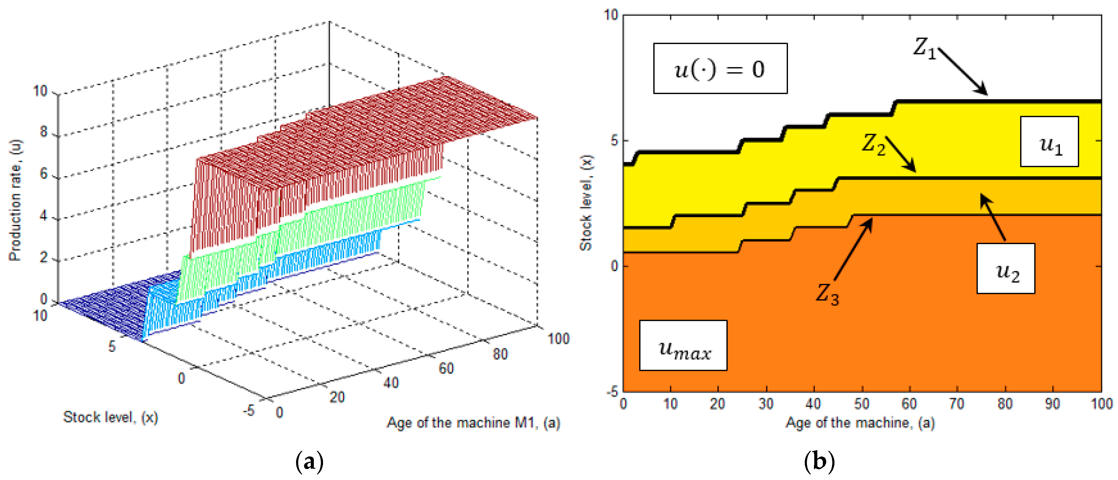
5.1. Production Policy

We present the obtained production policy $u^{*}(t)$ in Figure 5a. In such policy the production rate applied in the operational mode is defined in function of the system state that is determined in this case by the stock level and the age of the machine, ($x,a$). At examining this figure, we can realize that it exists a specific threshold for each production rate. To better interpret the production policy, we present its trace in Figure 5b. From the analysis of this figure, we have the following observations:

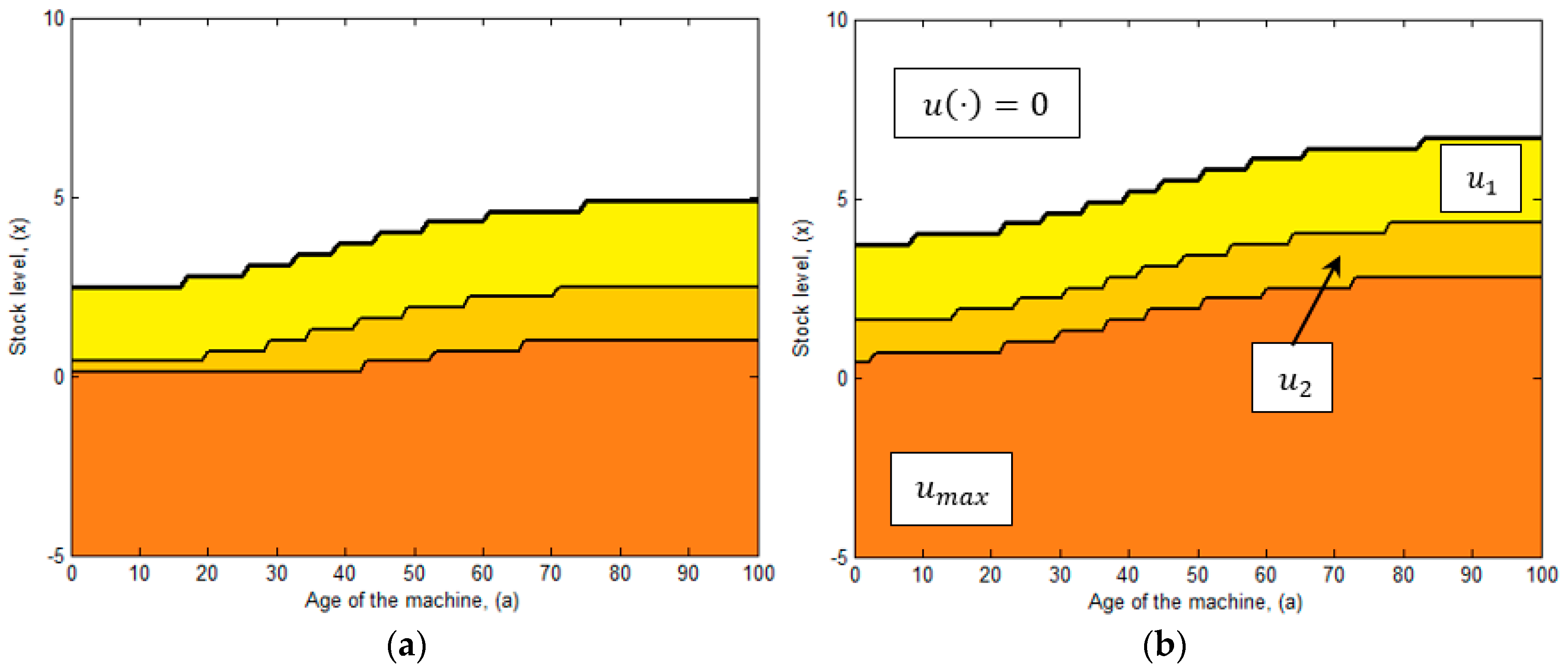
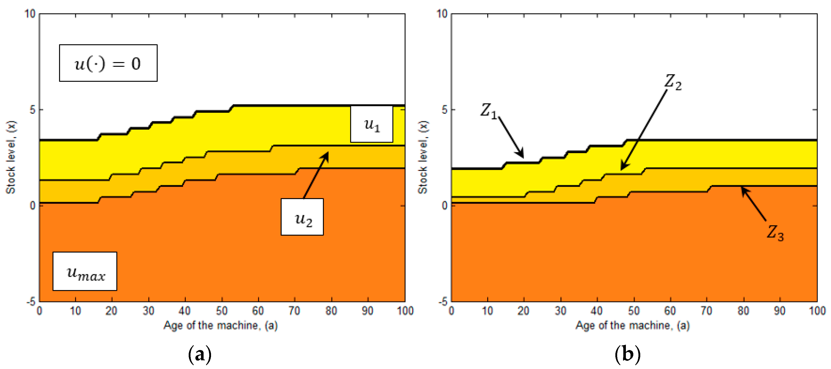
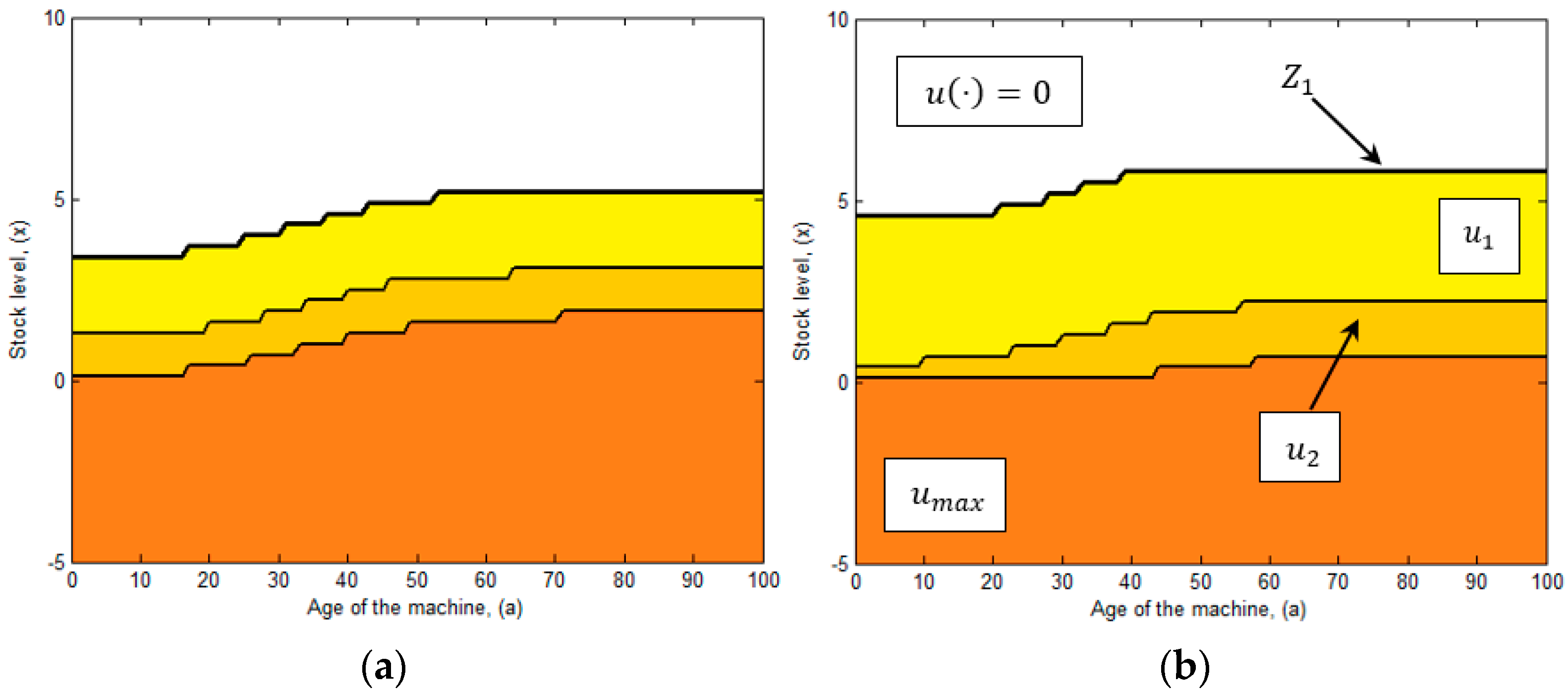
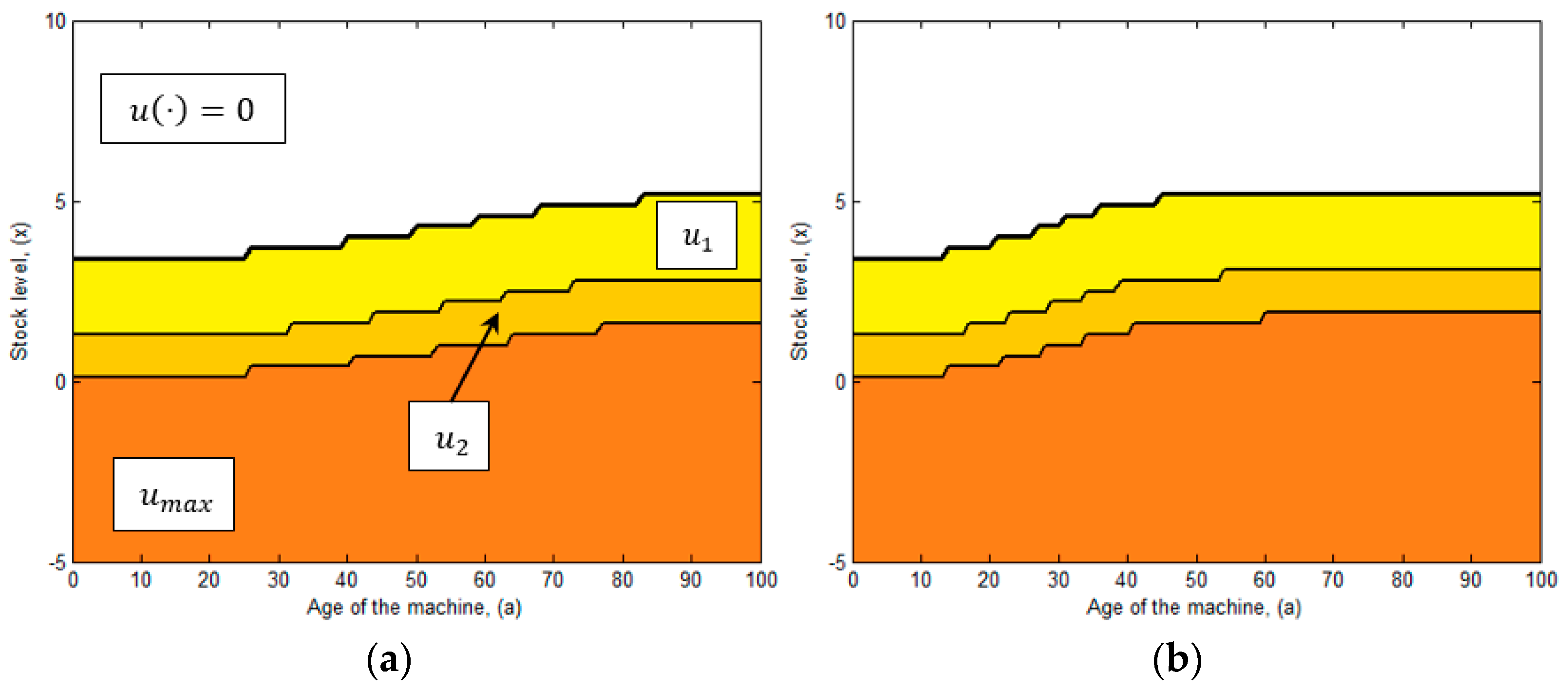
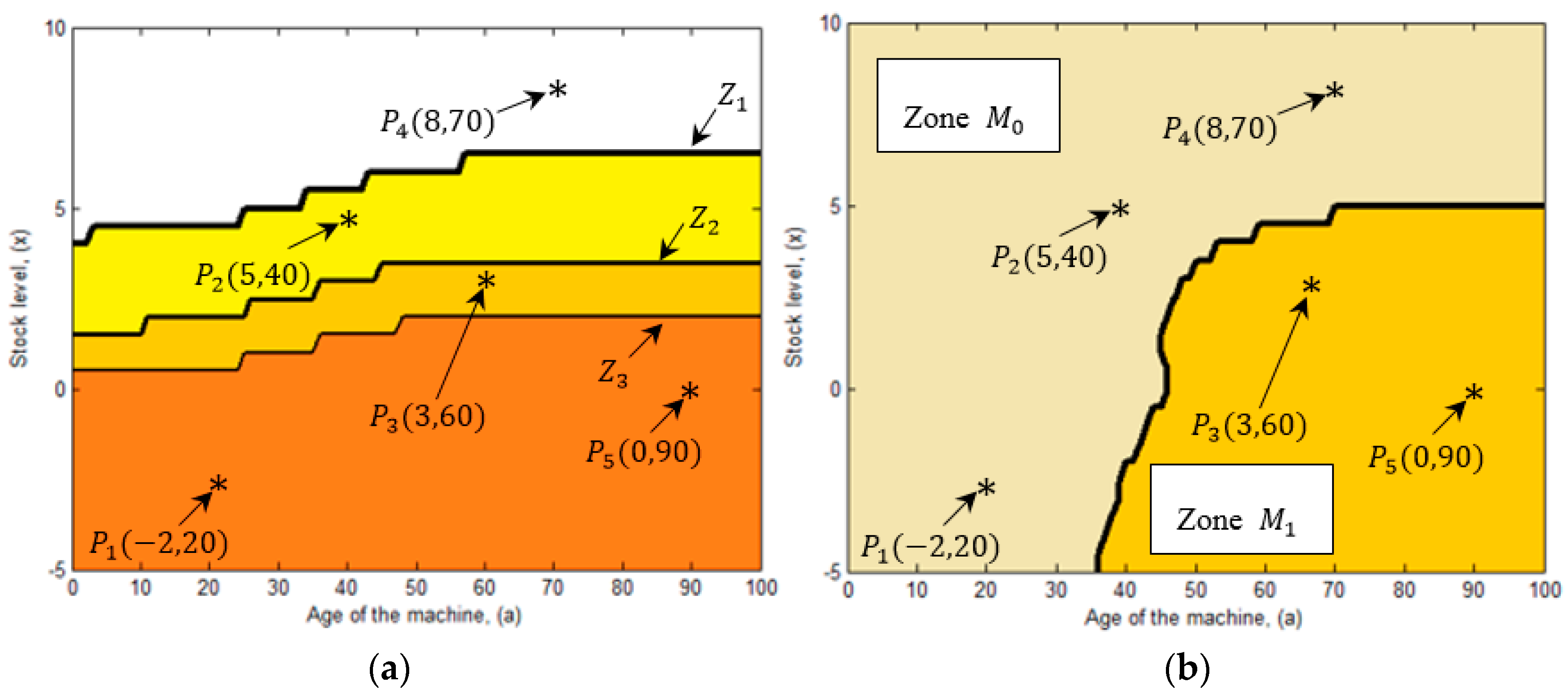
• The computational domain is divided in four zones, where the production rate is set to $0,u_1,u_2$, or $u_{max},$ respectively. Such zones are delimited by the production thresholds $Z_1,Z_2$, and $Z_3$.
• The production rate is decremented gradually (i.e., $u_{max}>u_2>u_1>0$) as the stock level increases and surpasses the production thresholds $Z_3,Z_2$, and $Z_1$ with $Z_1>Z_2>Z_3$. We note that the minimum production rate $u_1$ is recommended for high levels of inventory, when the stock level is between the production threshold $Z_1$ and $Z_2.$ Since given the existence of inventory, the system can manage to satisfy product demand operating at a reduced pace and mainly because it avoids further deterioration. Moreover, we note that as the stock level decreases, the production rate increases, thus the machine operates at its second production rate $u_2$ when the inventory level is between the thresholds $Z_2$ and $Z_3$, with the aim to replace inventory faster. Additionally, we note that the use of the maximum production rate $u_{max}$ is limited, because it deteriorates more rapidly than the machine, and so its use is only recommended in scenarios where the stock level is almost depleted and there is a need to rapidly replace the inventory level and avoid further shortages.
• From the obtained results we observe that the production thresholds $Z_1,Z_2,$ and $Z_3$ increases as the machine ages, this reflects the impact of the deterioration process on the production control rule. For instance at age $a=0$, the production threshold $Z_1$ has a value of $Z_1=4$, and as the machine deteriorates, at age $a=100$, such threshold increases to $Z_1=7$. The same pattern is observed for thresholds $Z_2$ and $Z_3$. The increment is explained by the fact that as the machine deteriorates, it produces more defectives and also it is subject to experience more frequent failures. Thus, more inventory is needed as protection to mitigate shortages.

Our results differ from the classical results of Kenné et al. [23] with only three production rules. In our case, the production policy defines the following control rules:

• Decrease the production rate to zero, if the current stock level is above the first production threshold $Z_1$.
• Set the production rate to its first productivity $u_1$, when the current stock level is under the first production threshold $Z_1$.
• Increase the production rate to its second productivity $u_2$, when the stock level is below the second production threshold $Z_2$.
• Increase the production rate to its maximum rate $u_{max}$, when the current stock level is under the third production threshold $Z_3$.

In a practical sense, the results of Figure 5 imply a multi-hedging policy form, where the production rate is defined as follows:

$$u{(1,x,a)}^{*}=\{\begin{array}{cc}\begin{array}{c}{u}_{max}\\ u_2\\ \begin{array}{c}{u}_1\\ 0\end{array}\end{array}& \begin{array}{c}ifx(t)<Z_3(·)\\ ifx(t)<Z_2(·)\\ \begin{array}{c}ifx(t)<Z_1(·)\\ ifx(t)>Z_1(·)\end{array}\end{array}\end{array}$$

(25)

where $Z_1(·)>Z_2(·)>Z_3(·)$ and $0<u_1<u_2<u_{max}$. Equation (25) incorporates the notion that it is advantageous to reduce the production rate from its maximum value to a more profitable level, since production at higher rates accelerates the machine degradation increasing then the total cost, and the economic performance of the unit may be compromised if the effects of such degradation are disregarded.

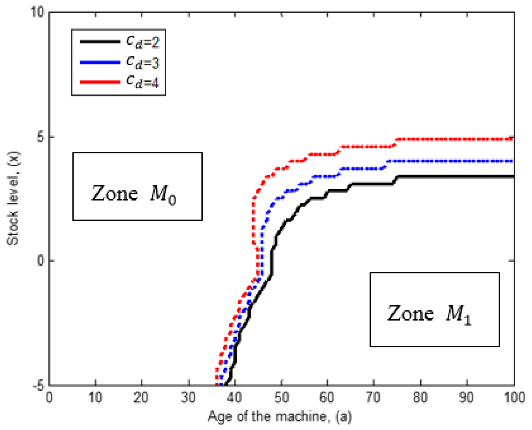
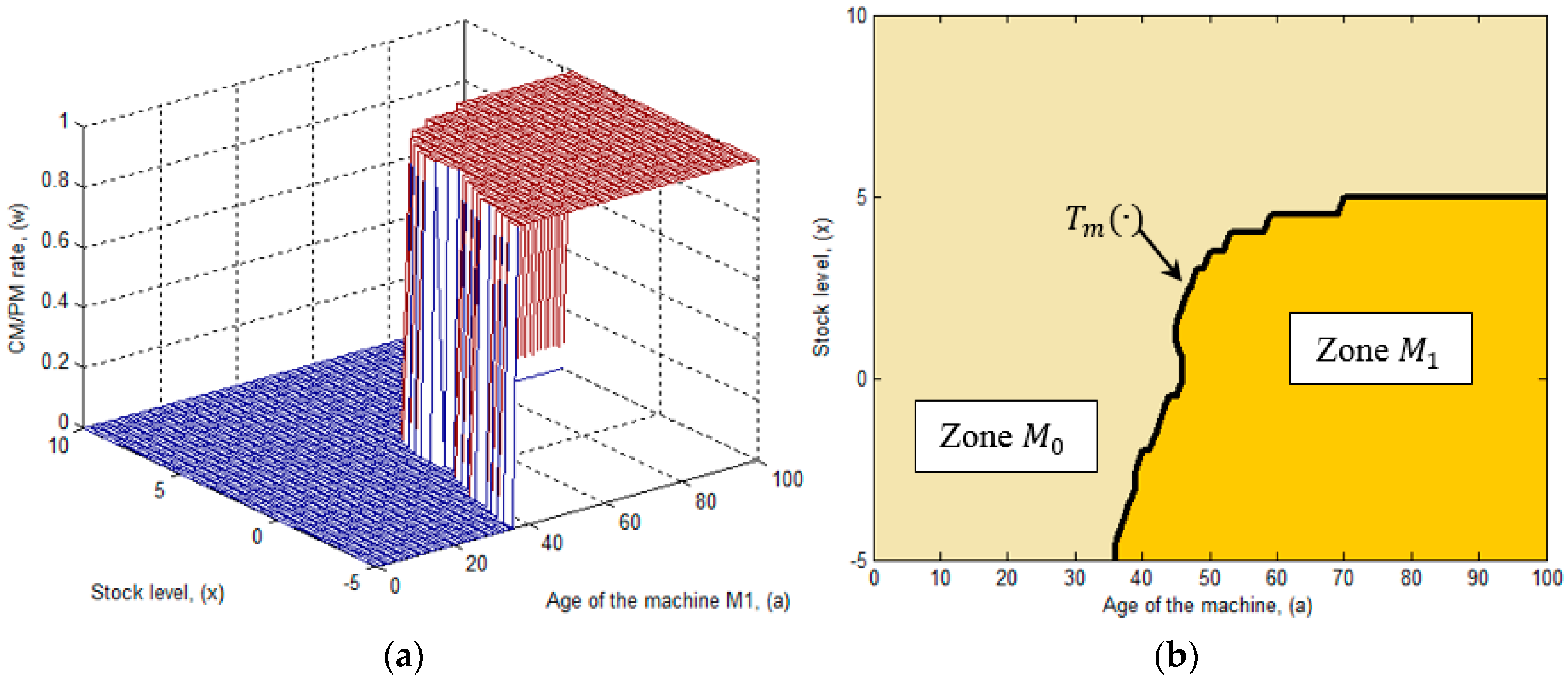
5.2. Repair/Major Maintenance Switching Policy

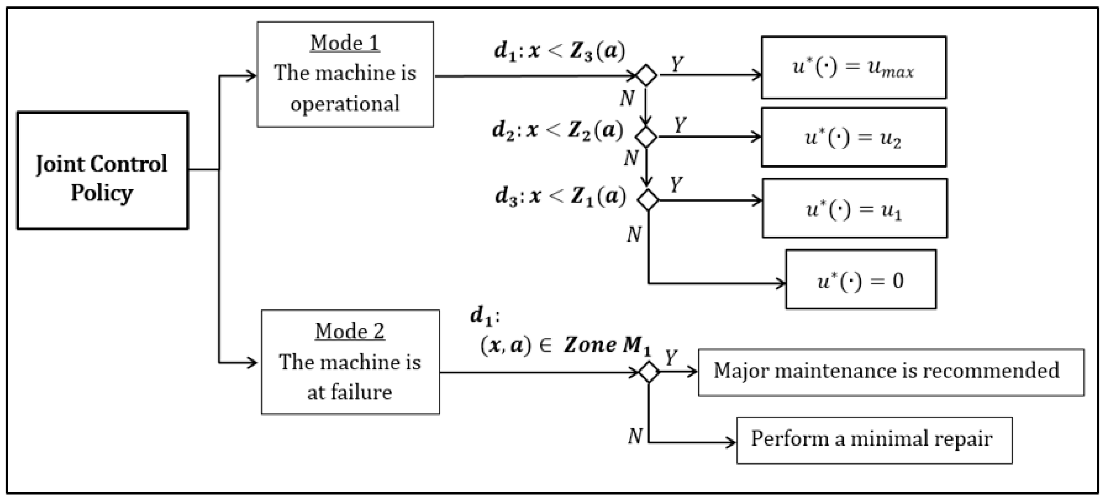
The repair/major maintenance switching policy is presented in Figure 6a. Once the machine is at failure we use the decision variable $w(t)$ to properly synchronize the two available maintenance options. The logic behind the maintenance strategy is as follows:

• When $w(t)$= 1, the variable is set to its maximum value, and it denotes the conduction of a major maintenance that completely mitigates the effects of the deterioration process, in this case reducing the failure intensity and the generation of defective units to initial conditions.
• When $w(t)=0$, the variable is set to its minimum value, indicating that a minimal repair must be performed. This type of maintenance does not restore the machine, since it leaves it the level of deterioration in the same level before the conduction of the repair.

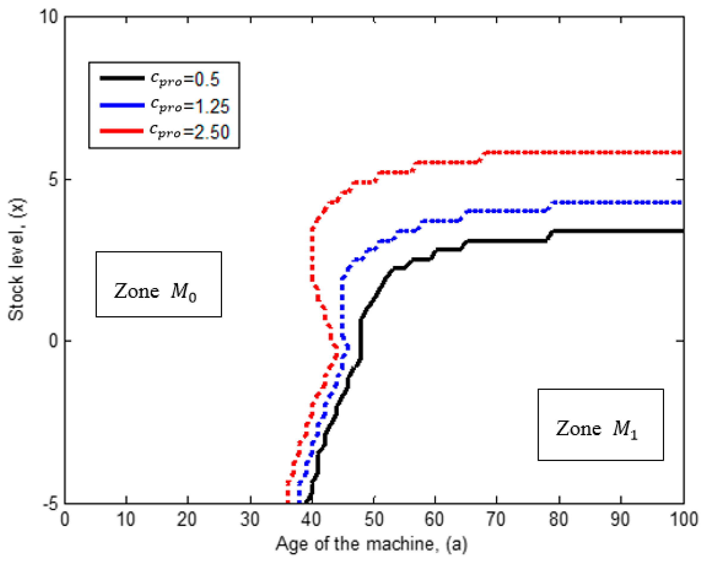
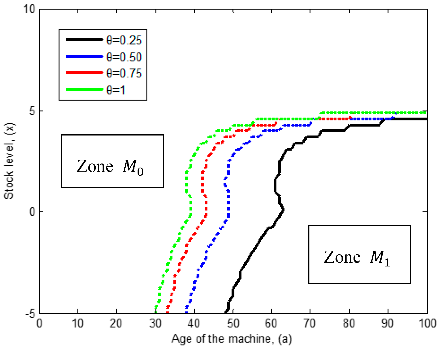
At observing the results of Figure 6a, we note that the computational domain is clearly divided into two zones indicating the type of maintenance recommended. With the aim to facilitate the characterization of the maintenance-switching policy, we present its trace $T_m(·)$ in Figure 6b. This trace serves us to define the following zones:

• Zone $M_0$: this zone suggests the conduction of a minimal repair, hence the decision variable $w(t)$, is set to its minimum value, $w(t)$= 0.
• Zone $M_1:$ in this zone the recommendation is to conduct a major maintenance, since given the level of deterioration of the machine is not profitable its operation. Thus $w(t)$ is set to its maximum value, $w(t)$ = 1.

Fundamentally, at analyzing the results of Figure 6b, it is evident that the level of deterioration of the machine is the key parameter to determine the maintenance strategy. In particular, we note that when the level of deterioration of the production unit is moderate, (i.e., between age $a=0$ and $a=35$ in Figure 6b) then the system opts to recommend a minimal repair and avoid further costs of the expensive major maintenance. However, when the machine reaches higher levels of deterioration (i.e., after age $a=35$ in Figure 6b) it is preferable to conduct a major maintenance than to experience the effects of more frequent failures and the increase of defective units. Thus, in our results, the repair/major maintenance activities are triggered according to a machine-deterioration-depended policy with a bang-bang structure, and it is given by the following expression:

$$w{(2,x,a)}^{*}=\{\begin{array}{c}\begin{array}{cc}1& if(a,x)\in Zone{M}_1\end{array}\\ \begin{array}{cc}0& if(a,x)\in Zone{M}_0\end{array}\end{array}.$$

(26)

In view of Equation (26), once the machine is at failure, major maintenance must be conducted only when the machine has reached a certain level of deterioration that justifies its expensive cost.

6. Sensitivity and Results Analysis

The operational validity of the model is discussed in this section through the analysis of different manufacturing scenarios consisting in the variation of several cost parameters. The purpose of this sensitivity analysis is to determine if the obtained joint control policy is confirmed and characterized consistently by the control factor $Z_i(·)$ and $T_m(·)$. The sensitivity of the proposed control policy is performed according to the variation of the inventory, backlog, repair, major maintenance, and defectives costs. Additionally, we also discuss the influence of an adjustment parameter of the trend of the failure rate.

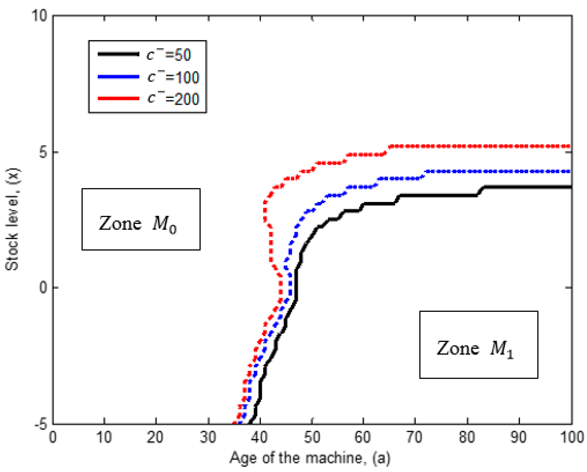
6.1. Influence of the Backlog Cost

The effect of the variation of the backlog cost on the production policy is presented in Figure 7, where we illustrate the production traces for two cost values, $c^{-}=50$ and $c^{-}=250$. From the obtained results, we realize that at reducing the backlog cost to $c^{-}=50$ the production thresholds are less extended on the computational domain. Then at increasing the backlog cost to $c^{-}=250$, the production thresholds increase as protections against backlog, since shortages are more penalized. The influence of the deterioration process on the production policy is evident, because the production thresholds increase as the machine ages. Additionally, we note that the machine operates at a reduced pace (i.e., zone $u_1$ and $u_2$) when there is some inventory, and the maximum production rate is devoted just in case of backlog or to maintain some protection stock when the machine reaches higher levels of deterioration.

Regarding the results of Figure 8, it is apparent that the backlog cost also influences the repair/major maintenance switching policy. For this cost parameter, we compared three cases, $c^{-}=50$, $100$ and $200$. In analyzing such scenarios, we notice that when the backlog cost decreases to $c^{-}=50$, major maintenance is less recommended, and so more minimal repairs are performed. If the backlog cost increases to $c^{-}=100,$ the major maintenance zone grows. Moreover, when the backlog cost is set to $c^{-}=200$, even more major maintenance is recommended. This increment is explained because at increasing the backlog cost, the effects of deterioration on shortages and defectives are more penalized. Hence, maintenance options that serve to mitigate effectively the effects of such deterioration, (as major maintenance), are more recommended. With respect to the inventory cost, we notice that is has the opposite effects that the backlog cost.

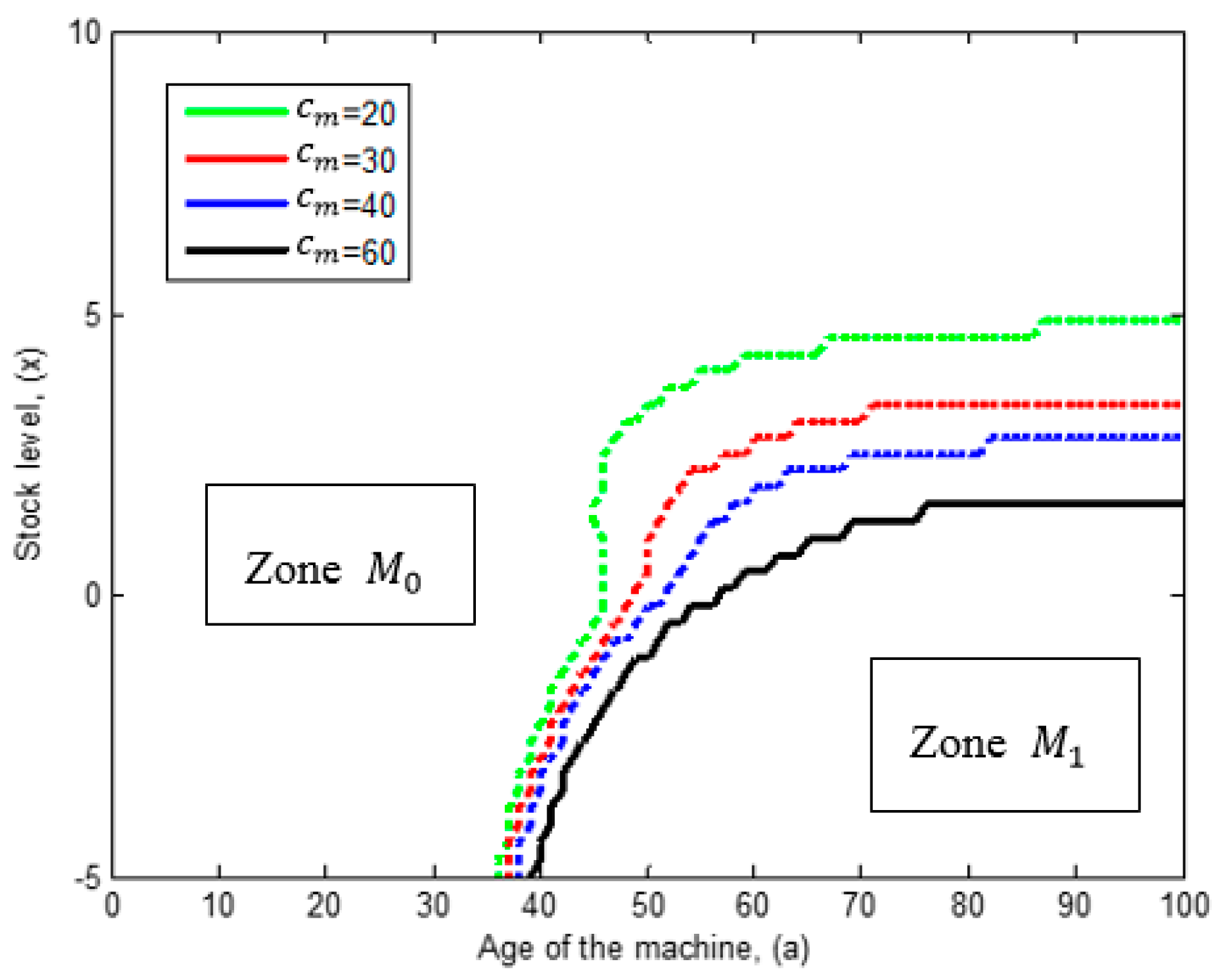
6.2. Influence of the Major Maintenance Cost

In discussing the sensitivity of the major maintenance cost, we examine four scenarios for the cost values $c_m=20,30,40$ and $60$. The obtained results are presented in Figure 9. When we set the major maintenance cost to a low value such as $c_m=20$ and $30,$ the maintenance policy indicates that the major maintenance zone covers a greater surface on the plane $(x,a)$. Nevertheless, if we increase the major maintenance cost to $c_m=40$ and $60$, minimal repairs are more recommended, reducing considerably the conduction of major maintenance. The observed pattern in the maintenance policy implies the fact that as beneficial and productive as a major maintenance can be, at increasing the $c_m$ cost, the machine must reach higher levels of deterioration to justify the expensive cost of such type of maintenance. Regarding the production policy, we observe that the major maintenance cost has no influence on this policy. Furthermore, that the minimal repair cost $c_r$ has the inverse effects of the major maintenance cost.

6.3. Influence of the Defectives Cost

We proceed with the analysis of the sensitivity of the defectives cost. In Figure 10 we analyze the production trace for two different cost values $c_d=3$ and $c_d=12$. From the results we highlight the fact that when the defectives cost is low, for instance $c_d=3$, there is more liberty to operate the machine at increased paces such as $u_2$ and $u_{max}$, regardless that in such rates the machine deteriorates faster, thus producing even more defectives. Moreover, we observe that when we increase the defectives cost to $c_d=12$, the production threshold $Z_1$ increases, favoring more the use of the machine at a reduced rate $u_1,$ (since at this mode the machine decreases considerably its deterioration pace, hence it generates less defectives). Additionally, it is evident that the greater the value of the defectives cost, the less extensive is the use of the machine at faster production rates such as $u_2$ and $u_{max}$. Because operating at faster production rates, the machine accelerates its deterioration level, generating more defectives.

To complement the analysis of the defectives cost, we examine its variation for three cost scenarios, $c_d=2,3$ and $4$ as illustrated in Figure 11. We begin the discussion when the defectives cost is set to a low value of $c_d=2$, in this context, the major maintenance activity is limited to the smallest area in the analysis. If the defectives cost increases to $c_d=3$, the repair/major maintenance trace varies and the area for the major maintenance increases. At increasing the defectives cost to $c_d=4$, minimal repair is less recommended, whereas the major maintenance zone increases even more. These results amount to the observation that the repair/major maintenance policy is highly sensitive to the defectives cost, since at increasing $c_d$, more major maintenance is conducted with the aim to restore the machine faster and reduce considerably the generation of defectives and at the same time maintain a reasonable total cost.

6.4. Influence of the Production Cost

The variation of the production cost $c_{pro}$ indicates that it has a strong effect on the production policy, as can be seen in Figure 12. For this cost we analyze two different cost scenarios with values $c_{pro}=0.5$ and $5$. If the production cost is reduced to $c_{pro}=0.5$, the production thresholds ($Z_1$, $Z_2$ and $Z_3)$ increase, because it is less expensive to operate the machine. By increasing the production cost to $c_{pro}=5$, the production thresholds ($Z_1$, $Z_2$ and $Z_3)$ reduce considerably. The reason behind this decrement is that at increasing the production cost, the system reacts by maintaining just the necessary amount of inventory to palliate shortages caused by failures and defectives units.

The production cost also influences the repair/major maintenance switching policy as observed on Figure 13. We use three different cost values $c_{pro}=0.5,1.25$ and $2.5$ for the analysis. The results of Figure 13 clearly indicate that major maintenance is less recommended when the production cost is set to a reduced value of $c_{pro}=0.25$. At increasing the product cost to $c_{pro}=1.25$, more major maintenance is conducted. Further, the zone for major maintenance expands even more at increasing the production cost to $c_{pro}=2.5$. To clarify matters, more major maintenance is recommended at increasing the production cost, because the operation of the machine becomes more selective, promoting more maintenance actions that mitigate completely the effects of deterioration $c_{pro}$.

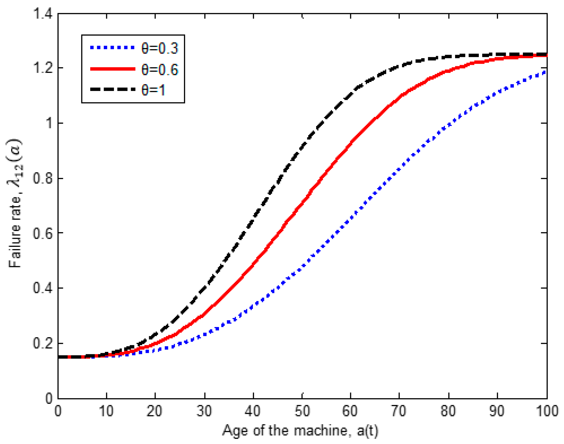
6.5. Influence of the Pace of the Failure Rate

We complement the sensitivity analysis with the analysis of the effect of the pace of deterioration of the failure rate. For this purpose, we examine the influence of the adjustment parameter $\theta$, which accelerates the failure rate of the machine. For this parameter, we examine two different scenarios with values $\theta =0.15$ and $1$, as illustrated in Figure 14. From the results, we note that whenever the adjustment parameter has a moderate value of $\theta =0.15$, the production thresholds have a smoother increment as the machine deteriorates. On increasing the adjustment parameter to $\theta =1$, the production thresholds reach its maximum values more abruptly. Another more pragmatic reason for this pattern is because with the increment of the parameter $\theta$, we are accelerating the pace of deterioration of the machine, and so the production thresholds increase earlier as protections against shortages and defectives.

A close examination of Figure 15 shows that the repair/major maintenance policy also is significantly affected by the variation of the pace of the failure intensity. To have a better understanding about such influence, we analyze four different scenarios with values = 0.25, 0.50, 0.75 and 1.00. From the maintenance traces presented in Figure 15, we realized that when the adjustment parameter is low, for instances $\theta =0.25$ and $0.50$ it implies that the system experiences less frequent failures, and so major maintenance is less recommended. There are more frequent failures when the parameter is set to a higher value such as $\theta =0.75$ and $1$, where more major maintenance is conducted. From this pattern, we can draw the inference that with higher values of the parameter $\theta$, we accelerate the pace of deterioration of the machine, and this promotes the conduction of more major maintenance to rapidly mitigate the effects of deterioration.

Throughout the discussion of the sensitivity analysis, we observe that the obtained joint control policy is significantly influenced by the deterioration of the machine. Furthermore, this sensitivity analysis allows us to state that the structure of the proposed control policy is consistent, and that such policy is well characterized by the control parameters $Z_i(·)$ and $T_m(·)$. At considering simultaneously in our integrated model, production planning and the repair/switching strategies, we seek to operate more efficiently the manufacturing system.

7. Comparative Study

The objective of this section is to compare the obtained joint control policy in order to illustrate the advantage of applying our approach in practice and highlight the economic benefit that decision-makers can obtain at implementing our joint strategy. We should note that the joint production and maintenance policies proposed in this paper have not been studied under the same assumptions of deterioration and operation-dependent defectives in the literature yet. However, we have managed to compare the total cost incurred from our joint control policy with the total cost reported from other policies based on assumptions common in the literature that does not takes into account the effects of deterioration on the control parameters. The policies considered in the comparison are described as follows:

• Policy-I: defines the production scenario (basic case) of the joint control policy obtained in Section 5, where the production and maintenance policies are determined simultaneously in an integrated model. The particularity of Policy-I is that the production threshold is dynamic, it is adjusted progressively in function of the level of deterioration of the machine, and major maintenance can be once the machine has reached a certain level of deterioration that justifies the cost of such type of maintenance. Thus, the conduction of major maintenance has a feedback on the level of deterioration of the machine.
• Policy-II: this policy is derived from the previous policy with the difference that the production threshold is not adjusted progressively, it remains constant at a given level for all the considered time interval and it does not evolve in function of the deterioration of the machine. Nevertheless, the conduction of major maintenance can be conducted based on a feedback with the deterioration of the machine as in Policy-I.
• Policy-III: the production threshold is dynamic and it is adjusted in function of the deterioration of the machine as in Policy I. However, major maintenance is conducted only when the machine has reached its maximum age limit.

Table 3. Cost difference of the comparative study.

Scenario	Production Threshold $\mathit{Z}$	Major Maintenance $\mathit{w}$	Optimal Total Cost	Cost Difference $\Delta (\%)$
Policy-I (basic case)	dynamic	feedback with deterioration	83.16	-
Policy-II	constant	feedback with deterioration	97.96	17.79%
Policy-III	dynamic	conducted at the age limit	113.40	36.36%

summarizes the different production scenarios considered in the comparison, it presents the total cost incurred when the level of deterioration of the system recommends the performance of a major maintenance and also such table presents the observed differences in the total cost. The results presented in Table 3, were obtained with the same data parameters shown in Table 1 and Table 2.

The interpretation of the obtained results of Table 3 implies that Policy-II reported a cost 17.79% higher than our joint control Policy-I, because Policy-II fails to consider the strong effect of the deterioration process on the production control rule. Maintaining a constant production threshold is not profitable in Policy-II, because it is evident that as the machine deteriorates it produces more defectives and also it is subject to more frequent failures. Thus, the production threshold must be progressively increased as a countermeasure to avoid shortages and ensure demand satisfaction with flawless units, as in Policy-I.

With respect to the total cost obtained by Policy-III, we noted that it reported a cost 36.36% more expensive than the cost of Policy-I. The observed cost difference is given mainly because the production and maintenance strategies in Policy-III are not determined simultaneously. In Policy-III, the production threshold are first determined taking into account quality and deterioration levels but with the disadvantage to disregard any consideration of the maintenance strategy. Thus, the obtained results indicate that it is not optimal to separate production and maintenance decisions because the delay of major maintenance increases the effects of deterioration in particular the defectives cost. It is evident that the obtained results support the need of an integrated model such as our Policy-I, that incorporates the strong inter-relationship between the key functions of production-quality and maintenance.

8. Managerial Implication

The obtained joint control policy of this paper is a derivation of the Hedging Point Policy that has been successfully implemented in real production systems as in the Boeing Flap Support Business Unit to control production strategies, as indicated in Gershwin [24]. Other implementation in a real production system, is reported by Dror et al. [25] to coordinate production and subcontracting strategies for a chemical company. In our case, the implementation of the obtained control policy in a real case needs complete information about the state variables of the production system, namely the inventory level and the age of the machine $(x,a)$. The benefit of the implementation of our control policy for the decision maker is that the policy permits to operate the production system more smoothly and predictably at scheduling properly production and maintenances rates. Moreover, our policy has the advantage to endure the effects of the set of disruptions encountered in real production (such as shortages, defectives, increasing failures, imperfect repairs, and deterioration).

The implementation of the obtained control policy is facilitated with the use of the implementation chart presented in Figure 16. This chart defines convenient actions that should be scheduled when the machines is operational and when it is at failure. In the implementation chart the control parameters $Z_1(·)$, $Z_2(·),Z_3(·)$ and $T_m(·)$ must be updated regularly as the machine deteriorates.

As an illustration of how to apply our joint control policy in practice, we determine the production and maintenance control rates for five different points located on the grid $(x,a)$ as presented in Figure 17, for the results obtained in the numerical example of Section 5.

The value of the control parameters are presented in Table 2 for the selected points ($P_1$ to $P_5$) of Figure 17. The value of such control parameters are determined by monitoring the state of the system $(x,a)$ by the implementation chart presented in Figure 16.

The logic of the policy is straightforward, for instance when the machine is operational in point $P_3$, the stock level is $x=3$ and the age of the machine is $a=60$, and so the machine must operate at $u_2=5$ because the stock level is less than the productions threshold $Z_2$ (i.e., $(x=3)<Z_2$) as indicated in Equation (25). Furthermore, once the machine is at failure, in point $P_3$ major maintenance is recommended, thus $w=1$, since the state of the system is inside Zone $M_1$, where the machine is so deteriorated that the cost of a major maintenance is justified. From the implementation of

Table 4. Implementation of the control policy.

Point	$(\mathit{x},\mathit{a})$	$\mathit{Z}$	${\mathit{u}}^{*}(·)$	${\mathit{w}}^{*}(\mathbf{·})$
$P_1$	$(-2,20)$	$Z_3$	$u_{max}=10$	$0$
$P_2$	$(5,40)$	$Z_1$	$u_1=2.5$	$0$
$P_3$	$(3,60)$	$Z_2$	$u_2=5$	1
$P_4$	$(8,70)$	$Z_1$	$0$	0
$P_5$	$(0,90)$	$Z_3$	$u_{max}=10$	1

, we notice that obtained joint control policy is practical for factory control, because of its ease to be implemented.

9. Conclusions

The number of scientific publications in the new field that analyses the strong interaction between production logistics, quality, and maintenance design is increasing steadily, reflecting the major relevance of this subject. However, most of the literature is based on systems that optimize either the production-maintenance or the production-quality relationships, leading to sub-optimal solutions. By contrast, this paper investigates the problem of determining the optimal production and repair/major maintenance switching maintenance strategies in the context of reliability and quality deterioration. In the manufacturing system under study, the rate of defectives depends on the production pace of the machine, defining operation-dependent defectives. We developed a stochastic optimization model where the joint production and maintenance control policies were determined by the resolution of the Hamilton-Jacobi-Bellman equations. From the obtained results it has been found when the rate of defectives depends on the production pace where the production policy defines a multi-hedging point policy with several production thresholds. Additionally, the results shows that in order to reduce the total incurred cost, it is beneficial to progressively decrease the production pace of the unit from its maximal value to inferior rates when there are no backlog in the system and there is a positive level of inventory. The results obtained promote major maintenance activities when the production unit reaches a level of deterioration that justifies the cost of an expensive maintenance. We illustrated and validated our proposed approach through a numerical example and an extensive sensitivity analysis. We discussed managerial implications for the decision maker at implementing our approach in real production systems. To further validate the model, a comparative study has been performed, where we noted that our approach represents a valuable alternative for controlling modern production units. Since we obtained cost economies of around 36%, at comparing our joint control policy with other strategies based on common assumptions of the literature that disregard the major interactions among production, quality, and maintenance. As a subject of future research, imperfect maintenance strategies could be integrated to the developed model in order to reduce the total cost and improve the profitability of the company.

References

1. Liberopoulos, G.; Papadopoulos, C.T.; Tan, B.; Smith, J.M.; Gershwin, S.B. Stochastic Modeling of Manufacturing Systems, 1st ed.; Springer: Berlin, Germany, 2006; pp. 3–363. ISBN 978-3-540-26579-5. [Google Scholar]
2. Colledani, M.; Tolio, T. Integrated analysis of quality and production logistics performance in manufacturing lines. Int. J. Prod. Res. 2011, 49, 485–518. [Google Scholar] [CrossRef]
3. Yedes, Y.; Chelbi, A.; Rezg, N. Quasi-optimal integrated production, inventory and maintenance policies for a single-vendor single-buyer system with imperfect production process. J. Intell. Manuf. 2012, 24, 1245–1256. [Google Scholar] [CrossRef]
4. Rivera-Gómez, H.; Gharbi, A.; Kenné, J.P.; Montaño-Arango, O.; Hernández-Gress, E.S. Production control problem integrating overhaul and subcontracting strategies for a quality deteriorating manufacturing system. Int. J. Prod. Econ. 2016, 171, 134–150. [Google Scholar] [CrossRef]
5. Mhada, F.Z.; Ouzineb, M.; Pellerin, R.; El-Hallaoui, I. Multilevel hybrid method for optimal buffer sizing and inspection stations positioning. SpringerPlus 2016, 5, 2045. [Google Scholar] [CrossRef] [PubMed]
6. Bouslah, B.; Gharbi, A.; Pellerin, R. Joint economic design of production, continuous sampling inspection and preventive maintenance of a deteriorating production system. Int. J. Prod. Econ. 2016, 173, 184–198. [Google Scholar] [CrossRef]
7. Midfal, I.; Hajej, Z.; Dellagi, S. Production/Maintenance Control of Multiple-Product Manufacturing System. In Proceedings of the Second World Conference on Complex Systems, Agadir, Morocco, 10–12 Novenber 2014. [Google Scholar] [CrossRef]
8. Khatab, A.; Ait-Kadi, D.; Rezg, N. Availability optimization for stochastic degrading systems under imperfect preventive maintenance. Int. J. Prod. Res. 2014, 52, 4132–4141. [Google Scholar] [CrossRef]
9. Hajej, Z.; Turki, S.; Rezg, N. Modelling and analysis for sequentially optimizing production, maintenance and delivery activities taking into account product returns. Int. J. Prod. Res. 2015, 53, 4694–4719. [Google Scholar] [CrossRef]
10. Askri, T.; Hajej, Z.; Rezg, N. Jointly production and correlated maintenance optimization for parallel leased machines. Appl. Sci. 2017, 7, 461. [Google Scholar] [CrossRef]
11. Martinelli, F. Manufacturing systems with a production dependent failure rate: Structure of optimality. IEEE Trans. Autom. Control 2010, 55, 2401–2406. [Google Scholar] [CrossRef]
12. Dahane, M.; Rezg, N.; Chelbi, A. Optimal production plan for a multi-products manufacturing system with production rate dependent failure rate. Int. J. Prod. Res. 2012, 50, 3517–3528. [Google Scholar] [CrossRef]
13. Haoues, M.; Dahane, M.; Mouss, K.N.; Rezg, N. Production planning in integrating maintenance context for multi-period multi-product failure-prone single-machine. In Proceedings of the 18th IEEE Conference on Emerging Technologies & Factory Automation, Cagliari, Italy, 10–13 September 2013. [Google Scholar] [CrossRef]
14. Kouedeu, A.F.; Kenné, J.P.; Dejax, P.; Songmene, V.; Polotski, V. Production and maintenance planning for a failure-prone deteriorating manufacturing system: A hierarchical control approach. Int. J. Adv. Manuf. Technol. 2015, 76, 1607–1619. [Google Scholar] [CrossRef]
15. Dong-Ping, S. Optimal Control and Optimization of Stochastic Supply Chain Systems, 1st ed.; Springer: London, UK, 2013; pp. 2–272. ISBN 978-1-4471-4724-4. [Google Scholar]
16. Love, C.E.; Zhang, Z.G.; Zitron, M.A.; Guo, R. A discrete semi-Markov decision model to determine the optimal repair/replacement policy under general repairs. Eur. J. Oper. Res. 2000, 125, 398–409. [Google Scholar] [CrossRef]
17. Gershwin, S.B. Manufacturing System Engineering, 1st ed.; PTR Prentice Hall: Englewood Cliffs, NJ, USA, 1994; pp. 1–501. ISBN 013560608X. [Google Scholar]
18. Hlioui, R.; Gharbi, A.; Hajji, A. Replenishment, production and quality control strategies in three-stage supply chain. Int. J. Prod. Econ. 2015, 166, 90–102. [Google Scholar] [CrossRef]
19. Kushner, H.J.; Dupuis, P.G. Numerical Methods for Stochastic Control Problems in Continuous Time, 2nd ed.; Springer: New York, NY, USA, 2001; pp. 2–475. ISBN 978-0-387-95139-3. [Google Scholar]
20. Gharbi, A.; Hajji, A.; Dhouib, K. Production rate control of an unreliable manufacturing cell with adjustable capacity. Int. J. Prod. Res. 2011, 49, 6539–6557. [Google Scholar] [CrossRef]
21. Dehayem-Nodem, F.I.; Kenné, J.P.; Gharbi, A. Simultaneous control of production, repair/replacement and preventive maintenance of deteriorating manufacturing systems. Int. J. Prod. Econ. 2009, 134, 271–282. [Google Scholar] [CrossRef]
22. Hajji, A.; Gharbi, A.; Kenné, J.P.; Pellerin, R. Production control and replenishment strategy with multiple suppliers. Eur. J. Oper. Res. 2011, 208, 67–74. [Google Scholar] [CrossRef]
23. Kenné, J.P.; Dejax, P.; Gharbi, A. Production planning of a hybrid manufacturing-remanufacturing system under uncertainty within a closed-loop supply chain. Int. J. Prod. Econ. 2012, 135, 81–93. [Google Scholar] [CrossRef]
24. Gershwin, S.B. Design and operation of manufacturing systems: The control point policy. IIE Trans. 2000, 32, 891–906. [Google Scholar] [CrossRef]
25. Dror, M.; Kenneth, R.S.; Candace, A.Y. Deux chemicals inc. goes just-in time. Interfaces 2009, 39, 503–515. [Google Scholar] [CrossRef]
Figure 1. Manufacturing system under study.
Applsci 08 00165 g001
Figure 2. Transition diagram.
Applsci 08 00165 g002
Figure 3. Defectives rate.
Applsci 08 00165 g003
Figure 4. Increasing failure rate.
Applsci 08 00165 g004
Figure 5. Production policy. (a) Production rate; (b) Production trace.
Applsci 08 00165 g005
Figure 6. Repair/major maintenance switching policy. (a) Repair/major maintenance rate; (b) Trace of the repair/major maintenance policy.
Applsci 08 00165 g006
Figure 7. Sensitivity of the backlog cost on the production policy. (a) c = 50 ; (b) c = 250 .
Applsci 08 00165 g007
Figure 8. Sensitivity of the backlog cost on the repair/major maintenance policy.
Applsci 08 00165 g008
Figure 9. Sensitivity of the major maintenance cost on the repair/major maintenance policy.
Applsci 08 00165 g009
Figure 10. Sensitivity of the defectives cost on the production policy. (a) c d = 3 ; (b) c d = 12 .
Applsci 08 00165 g010
Figure 11. Sensitivity of the defectives cost on the repair/major maintenance policy.
Applsci 08 00165 g011
Figure 12. Sensitivity of the production cost on the production policy. (a) c p r o = 0.5 ; (b) c p r o = 5 .
Applsci 08 00165 g012
Figure 13. Sensitivity of the production cost on the repair/major maintenance policy.
Applsci 08 00165 g013
Figure 14. Sensitivity of the pace of the failure rate on the production policy. (a) θ = 0.15 ; (b) θ = 1 .
Applsci 08 00165 g014
Figure 15. Sensitivity of the pace of the failure rate on the repair/major maintenance policy.
Applsci 08 00165 g015
Figure 16. Implementation chart.
Applsci 08 00165 g016
Figure 17. Implementation chart. (a) Trace of the production policy; (b) Trace of the repair/major maintenance policy.
Applsci 08 00165 g017