Chaotic Synchronizing Systems with Zero Time Delay and Free Couple via Iterative Learning Control


Institute of Electrical and Control Engineering, National Chiao Tung University, Hsinchu 30010, Taiwan
*
Author to whom correspondence should be addressed.
Appl. Sci. 2018, 8(2), 177; https://doi.org/10.3390/app8020177
Submission received: 30 October 2017
/
Revised: 10 January 2018
/
Accepted: 23 January 2018
/
Published: 25 January 2018
(This article belongs to the Special Issue Selected Papers from IEEE ICASI 2017)
Abstract
:This study aims to orchestrate a less restrictive learning controller by using the iteration-varying function, the so-called iterative learning controller (ILC), to synchronize two nonlinear systems with free time delay and couple free. The mathematical theories are proven rigorously and controllers are developed for system synchronization, and then an example is forged to demonstrate the effectiveness of synchronization by the designed ILC. The ILC is designed with a feed-forward based by the error dynamics between the two considered nonlinear drive and response systems. The stability of the synchronization facilitated by the designed ILC is ensured by rendering the convergence of an error dynamics that satisfied the Lyapunov function. The Lorenz system within a drive-response system is considered as one system that drives another for the demonstration of the effectiveness of the designed ILC to achieve synchronization and verified initial conditions. Simulations are conducted for the controlled Lorenz system, and the results validated well the expected capability of the designed ILC for synchronization and matched the proposed mathematical theory.
1. Introduction
The method of Iterative Learning Control (ILC) was applied to mechanical robots in 1984 for performance improvement. The improvement is made possible by designing an on-line iterative learning scheme based on a classical linear system that approximates well the original nonlinear system of the robots. The approach of this on-line-learning ILC is of course very different from other known approaches, such as repetitive control, adaptive control, and the neural network [1,2]. The essence of on-line learning lies in the attribute of the controller that adapts its controller effort continuously based on the error feedback from the output of the system in an on-line fashion [2,3,4]. This ILC control method is applicable to many industrial systems for manufacturing, robotics, and assembly line in mass production [2,3]. Recently, the ILC theory was employed for chaos synchronization to stabilize communication protocols of encrypting and decrypting a message using dynamical filters, which are bi-directional over unidirectional coupling schemes of Bernoulli units, towards the tap-proof transmission of information via chaotic laser systems [5,6]. Due to the aforementioned value, the ILC for chaos synchronization was also intensively studied by academics [5,6]. Different types of controllers were developed, such as a proportional-integral-derivate (PID)-type ILC applied for improved robotic operations [3,7]. Also, ILC was employed for dynamical system synchronization based on classical linear system theory [8,9,10,11].
The Lyapunov criterion that served to guarantee the designed slave system in asymptotical synchronization with the master system in [12] is a common strategy that is used to study the stability of a control system. The principle of the learning operator is described in Hauser [13], and the Lyapunov function of the synchronization system pursues the method by Zhou [14] for stability. The Lyapunov function exhibited in [15,16,17,18,19,20,21] forms the criteria of the restrictive system with couple and time-delay to synchronize, the existence and stability conditions of two different continuous chaotic systems, and the synchronization manifold of two unidirectional systems, respectively.
The synchronized system analyzing was similar to the generalized Lorenz systems by coupling linear state error feedback control with coupling matrix to eliminate the given chaotic dynamics synchronization [22]. The controller is considered the linear combination of error dynamics feedback without the coupling matrix and previous learning rule to approach chaos synchronization [23]. The stable synchronization of a multi-chaotic network system was a single direction of the response system with error feedback non-coupling and was dependent on the eigenvalues of different time-delay coupling matrices between systems in [24]. The Iterative Feedback Tuning (IFT) method [25,26,27] was addressed to approach the optimization of the parameters of the controller and avoid replacing the bias information of the signal of the system. Therefore, the isochronal phenomenon of the non-linear secure communication system synchronization has been investigated in, along with several activities in nature [25].
This article employed an ILC law to design the controller, which is similar to adding a filter before the input of the system, and to synchronize two nonlinear systems with a distinct initial condition. The feed-forward control signal is an appropriate tracking reference that could achieve a low tracking error between systems to approach the synchronization of systems. The ILC method has only been applied to trace the trajectory of the robotic system and academic field over the past few decades.
The goal of this paper was not only to study the characteristics of the parameters in the synchronization process of the system, but also to apply the results into a secure communication system, as well as a traced robotic movement. This paper emphasized the “Learning” process and the behavior of parameters in the synchronization system. The “Learning” process in this article was to avoid too much matrix computing such as the linear matrix inequalities (LMI) method, to make it easy to find the controller for the system, and to adjust the fault-tolerant of the system, but differently from the iterative control process of the other studies, which emphasized periodic control. The proposed concept was verified by an identical drive-response system with a different initial condition. The rigorous proof and relevant mathematical theory was to prove the non-increasing bounded ILC law, the stable error dynamical system, and the convergent tracking error between systems. The results of the example in this paper indicated the behavior of the parameters in the synchronization process. The generalized Lorenz system, as a numerical synchronization example of nonlinear drive-response systems, is discussed in [22,27,28,29]. The chaos synchronization with undistinguished input and the reconstructing chaotic system by evolutionary algorithm also used the Lorenz system in [30,31].
The relevant studies herein include the following: (1) generic synchronization systems formulation; (2) proposing the related mathematical theory and the scheme of ILC; and (3) the simulation results by example to verify the proposed theory and exhibit the performance of the ILC algorithm. Finally, this paper derives a conclusion and a recommendation for future works.
2. The Iterative Learning Control (ILC) Problem Formulation
2.1. System Description
The drive and response systems are chaotic systems to synchronize with zero-time delay and couple free. The general formulas of systems are described by Equations (1a) and (1b), respectively.
The response system adjusts the error between the drive and tracking systems to synchronization by the control input.
The state vectors and and the outputs and are of the drive-response systems in the state space of , respectively. Originally, and weresimilar systems. The response system includes the iterative control input signal ofand the output, after the k-th learning of iteration. The Cm, Cs, and B = BT are non-singular constant matrices with appropriated dimensions and some entries of the nonsingular polynomial matrix are replaced by the i-th component of ,which is the factor of system synchronization, in which i = 1, 2, 3. The input signal sequence in is the control learning law after the k-th iterative learning for the response system synchronizing the drive system.
is the synchronization error and the output error of the drive-response system is given. The output error is equal to the synchronization error when is set.The dynamical system synchronization error between the drive-response systems is described in Equations (1a) and (1b).
The appropriateis given and subtracted in Equation (2) to beabsorbed by B. The limitation of synchronization error must approach zero, that is, , and the error dynamics should be less than or equal to zero, that is, , when the iteration learning procedure is applied to the response system to track the drive system in the time interval [0, T] after a sufficiently large iterative number, k.
The characteristics between the drive and response systems are that the drive system is a reference system and the tracking system is a response system in the synchronization procedure, respectively. The response system traces the trajectory of the drive system by employing the output information of the drive system. To achieve the goal of synchronization and search a system whose trajectory is close to the drive system, it is necessary to find an estimated system similar to the drive system. The estimated system in [21] can be defined by the measuring system of the drive system as shown in Equation (3).
The nonlinear problem has no general solution. The perturbation and linearization techniques will be applied to Equation (3). The least square linear estimation is familiar to minimize the errors in measurement processes. The error criteria of Equation (3) is defined as
The minimization of E is to differentiate E with respect to the state vector and equal to the results:
The parameter is the minimum value of the scale of error E.
The design of the Lyapunov function reaches the synchronization of the chaotic system in which the manifold must be stable [14,15,16,17,18].This fact indicates the system’s synchronization of Equations (1a) and (1b) through the ILC procedure so that the error dynamics Equation (2) are stable by the Lyapunov criteria and the local Lipschitz condition is satisfied during the period of the system.
Lemma 1.
Equation (2) has a trivial solution by the ILC procedure Equation (1a) and in Equation (1b) are satisfied by the local Lipschitz condition in the interval [0, T].
Proof.
By the ILC procedure, there is a trivial solution, which implies δ > 0 for all ε > 0 and k = 0, 1, 2, … such that as , which means the condition isheld. The isconvergent to when approaches zero. The consequence of this lemma implies that .
The convergence of the synchronization error, , indicates the error dynamicsas non-increasing, that is , and is dependent on the iterative learning control law, in Equation (1a) is chosen as:
in whichand are appropriate constant matrices and symmetry. The learning lawis prior to , and are the errors between the estimated state vectors and the state vectors of and, respectively.□
The sum of errors of Equation (6) is . If the error dynamics in Equation (2) is convergent then the iterative learning control law is decremented. The completed proof is exhibited in Lemma 2.
Lemma 2.
If the error dynamics in Equation (2) are convergent, then the iterative learning control law in Equation (6) is anon-increasing function.
Proof.
From Equation (5) and Lemma 1, the error in Equation (2) can be rewritten as follows
Suppose that and take the ; Equation (7) can be rewritten in detail as. The difference of iterative learning control law is , which means the sequence is non-increasing as the erroris convergent to zero.
The analytical approximation of the chaotic systems synchronizing the trajectoryin Equations (1a) and (1b) is to investigate the Lyapunov stability in [14,15,16,17,18]. The Lyapunov criterion introduced in Theorem 1 is a positive-definite function with no-time delay and couple free of the system (Equation (2)).□
Theorem 1.
The iterative learning control law is chosen as Equation (6). The Lyapunov function can be defined as
- (a)
- When is the Lyapunov function of an estimation system in the system (Equation (3)).
- (b)
- Ifis Lyapunov function of the system (Equation (2)), then the system should bestable.
Proof.
The proof of part (a) in the theorem has been proven. The derivative of the function along the track of the system (Equation (2)) is in [28], the discussion and written as
By using Lemma 1, Equation (9) has a trivial solution. The derivative of a Lyapunov function is equal to zero or negative, which implies that the system (Equation (2)) is stable.
Next, the proof of part (b) is a general case of a chaotic system with no time-delay and couple free. The derivative of the function along the track of the system (Equation (2)) is introduced in [14,15,16,17,18] and followed as:
The first term in Equation (10) is proven in Equation (8), and the second term should be equal to zero or negative when the iterative learning control law is a non-increased function. When the iterative control learning is divergent, the Lyapunov function of the dynamical system (Equations (1a) and (1b)) would be divergent and the system (Equation (2)) is not stable.□
In the proof of the theorem, it is important to determine the learning control law, u(k)(t), in the Lyapunov function applied in a more complex system. The decision was the most appropriate for iterative learning control law and parameters B1 and B2 to reduce the divergence of non-linear systems; this should be discussed and studied for the synchronization of non-linear systems.
2.2. Proposed Algorithm for Iterative Learning Control Law
The iterative learning control algorithm is exhibited in Figure 1. The diagram contains three systems: drive system, the response system, and the estimated system, with three outputs, namely the output of the drive system, the output of the response system, and the output of error, respectively. The initial conditions of the drive system and the response system are different. The iterative learning control law of the first stage exhibits the error of initial conditions between the drive system and the response system. The estimation system in Equation (3) provides for the estimated state vectors as expressed in Equation (4), the drive and response systems, respectively. The drive system and the response system are closed-loop so that the feedback in the former is its own output of the drive system, and the feedback in the latter is the result of iterative learning control law as its own output of the response system.
The algorithm in Figure 1 examines the learning control input u(k), which is bounded and convergent, satisfying the criteria of monotonically convergent conditions. The learning control input u(k) in Equation (6) is concerned with the ability to adjust the feedback error of the response system and track the trajectory of the drive system. Therefore, the iterative learning control law, u(k), must be bounded.
Corollary 1.
The learning control input u(k) in Equation (6) is a non-increasing and bounded function.
Proof.
The learning control law in Equation (5) is an updated law to refresh the input of the system (Equation (1b)) proposed. The sequence is a non-increasing sequence such that the condition is held with an upper bounded M of the real number in Lemma 2.
The appropriate matrices B, B1, and B2 making the sequence , being strictly decreasing are important. The ILC law can be expanded in the initial learning lawby induction as follows:
The consequence is from the monotonically decreasing sequence of the ILC rule. The u(0) is the maximum in the monotonically decreasing sequence and in Equation (13). Theses matrices can be found by the Linear Matrix Inequality (LMI) method, but were not the object in this research.□
3. Example Illustration and Demonstrated Results
The chaotic system reconstruction of unknown inputs has been developed in [32]. The ILC method could also be employed to track the trajectory between systems unknown reference [1,2,3]. The example in this article has two identical Lorenz systems; one of them is a reference system and another one is a tracking system. The generalized Lorenz systems have been the most studied under various conditions such as a standard Lorenz system, Chen system, Lü system, and unified chaotic system [22]. The Lorenz system has been widely introduced as a possible way to investigate chaotic dynamics and synchronization [27,28,29,31]. Therefore, the Lorenz system is capable of reconstructing chaotic systems by an evolutionary algorithm and verifying the chaos synchronization simulated by secure communications with unknown inputs [30,31].
The example in this section demonstrates the results of the synchronization approach, investigated to synchronize the non-linear drive-response systems with free time-delay and non-couple. A drive system was expressed by a Lorenz system following [28], and the response system is shown as another with the ILC input. In the synchronization approach, the ILC information was from the error dynamics of the desired-response system. The controller was designed by the ILC rule after collecting previous information. The Lyapunov function provided sufficient conditions for convergence to approach synchronization systems. The tracking error between the systems was an asymptotically stable system and a bounded function was constructed by a Lyapunov function. Next, the synchronization approach is shown.
3.1. The Example of Iterative Learning Algorithmto Decide Learning Law
To exhibit the synchronization of two non-linear systems and verify the algorithm of iterative learning control law in Figure 1, the drive-response systems with non-identical initial conditions are given by the following:
and
From the drive-response system, the dynamical error system is expressed as
In this example, given, the output error is in R3. The parameters are explained as , and . The in polynomial matrix is the first component of the state vector in the drive system. The state vector in the estimation system isand the iterative learning law with the initial condition. Thein Equation (6) and the Lyapunov equation are respectively shown as Equations (6) and (8).The matrices B1 and B2 in the ILC rule of Equation (6) are:
The matrix B2 is from the decomposition of the coefficient matrix of the system in (Equation (14)) and the matrix .The parameters and the matrix is in [33]. The matrix B in Equation (1b) is to select the identity matrix. The results were simulated by MATLAB (R2013b, Math Works, Natick, MA, USA, 2013) to verify the performance of the ILC rule. The drive system used the ode45 function in Simulink of MATLAB, and the response system used the Euler method with the estimated state vectors in Equation (5).The relevant simulation results are shown in the next section.
3.2. Simulation Results and Discussion
Figure 2 shows that the trajectories in the two-dimensional x1, x3-spaceofthe drive system are in the red line; the response system as the tracing system is in blue.
The drive system with initial condition, , differs from the response system, . The difference between the drive and response systems was larger than in other articles in which the initial condition alteration of a drive-response system was closed or not mentioned as in [12,13,14,15,16,17,18]. The trajectory of the response systems quickly approached that of the drive system after their initial condition and the approximation nearby the drive system, just as the iterative learning-controlled law containing the information from the drive system dominated the response system along the trajectory of the drive system.
According to Equation (2) and Lemma 2, the convergent error dynamics should be less than or convergent to zero, and the behavior is demonstrated in Figure 3. The components in were convergent to zero with averages of [−0.01341, −0.0122, and −0.1796] for each state of the system, respectively, satisfying the error convergent criterion. Three state vectors of error dynamics were vibration in the bounded interval as well, to verify the bounded error of each iteration and to design an appropriate controller by the ILC rule in Equation (2) and Lemma 2.
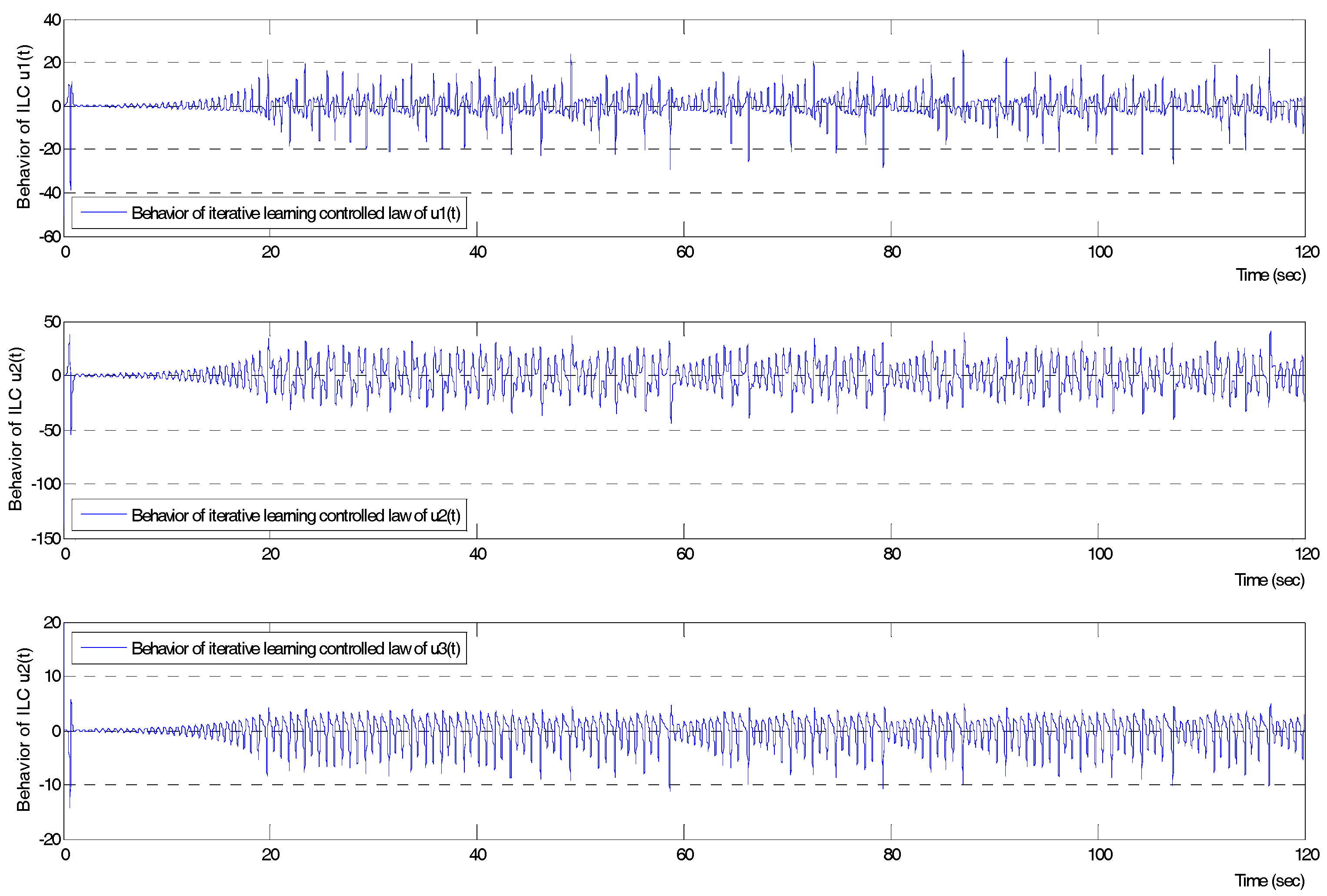
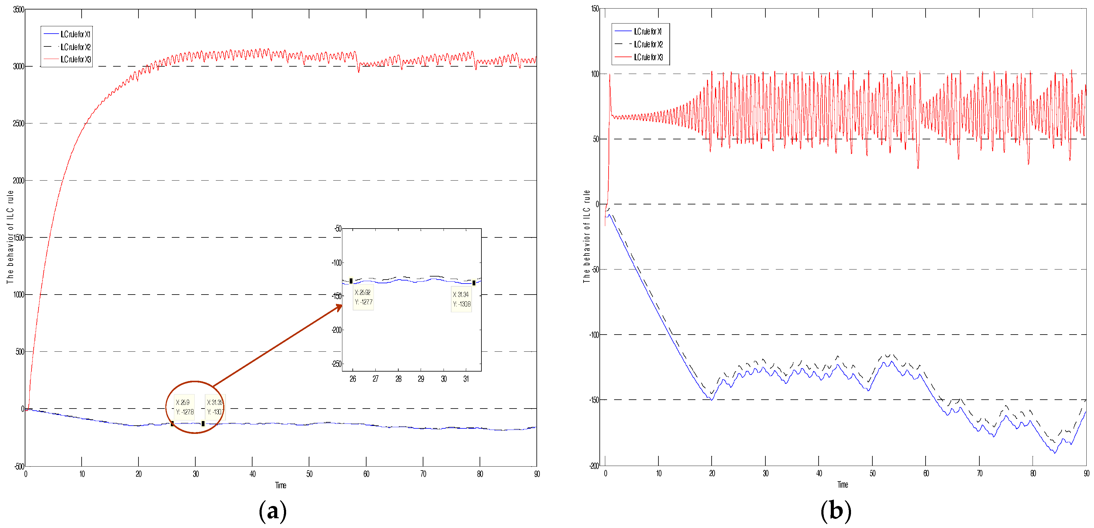
The behaviors of the ILC rule in Figure 4 show that the three components were always non-increasing and approached zero, and exhibited that the components were zero-central vibration in a bounded interval with average [–0.00919, 0.00171, −0.00469]. According to Equation (6), when the tracking error is an approximation to zero, the ILC law should approach zero in Lemma 2 and be a non-increasing and bounded function in Corollary 1. The simulation results of Equation (6) have already examined Lemma 2 and Corollary 1. The behaviors were not always identical to different ILC rules as shown in Figure 5. It is an important issue and challenges to select an eligible ILC rule. In Figure 5a, the B1 in Equation (6) was chosen as the identity matrix, and B1 in Figure 5b as a diagonal matrix [0.1, 0.1, 0.92]. In both Figure 5a,b, one of the components rose sharply and continued to vibrate in a bounded interval. Although the other components gradually decreased in the previous ILC rule, the ILC rule still makes the response system under an unpredictable situation.
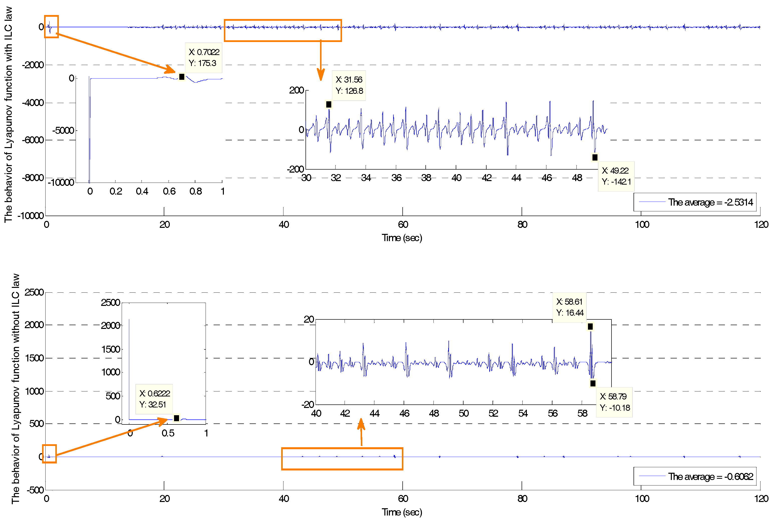
The behavior of the derivative of the Lyapunov function is demonstrated in Figure 6 and corroborates both Theory 1 and Lemma 2 by Equations (11) and (12). The data in Table 1 is the derivative of the Lyapunov function to count the number in which the value of the Lyapunov function in this article was zero or negative. The number in Table 1 was the closed relative to the different parameters μ in Equation (10). From the average in the table, most of the values of the Lyapunov function tended to be negative. Hence, the average of values of the Lyapunov function became positive when μ < 0. The most significant phenomenon was to regard the ILC rule to find an appropriate linear combination in Equation (6), and the derivative of the Lyapunov functionin Equation (10) was negative. The Lyapunov function is a non-increasing function by the conditions of Lemma 2 and the corollary, as seen in Figure 6, which shows the consequences and proves Theorem 1. The curve in Figure 7 demonstrates the behavior of the learning operator of the ILC rule by using the formula in Equation (12) in the blue line is the criterion of learning operator as Equation (13). Figure 6 shows the operator decreases rapidly to stability and verifies both Equations (12) and (13).
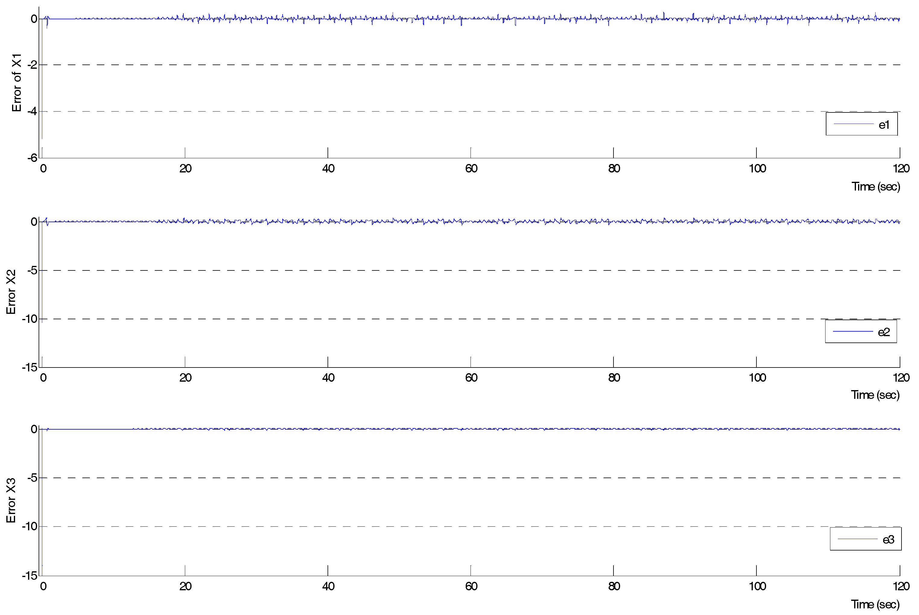
Next, Figure 8 shows the synchronization error for each component of the systems in Equations (15) and (16). The synchronization error of each component indicated that it was convergent to zero and vibrated in the neighborhood of zero. The average of the synchronization errors in 12,000 time steps were (–0.00049, –0.00077, and –0.00199) for each component. The exhibition of vibration in Figure 8 matched all components in Figure 3, in which the error dynamics should be convergent to zero when the tracking error approaches zero.
On the other hand, the situation of Figure 8 exhibits that the chosen ILC rule may be improved to reduce the vibration in the future so that the synchronization error maintains no vibration, but the synchronization error results were better than the other papers [4,14,15,16,17,18,19] and at least as good as [12,26,27]. This example has not only verified the concept in this paper, but it has also demonstrated the simulation results of the parameters in non-linear system control fields, providing the average of each parameter, which has not yet been completely discussed in other papers.
4. Conclusions
This research exhibited the design of an iterative learning controller and the results of the simulation with an example to prove the mathematical theory of the chaotic system synchronization via the iterative learning control law. The demonstrations verified the mathematical theory as able to approximate the synchronization between systems. The ILC method is a convenient method to trace the trajectory of systems, but is not a perfect tracking for all situations. In addition, the iterative learning control law should be conditionally dependent on the system and would not be unique to the specific system. It was a significant challenge to find coefficient matrices that were the combination of the previous ILC law and the trajectory error in this research, respectively. Finally, the example in this article has not only verified the theory and concept in this paper, but also demonstrated the behavior of parameters in non-linear system control fields, which has not yet been completely discussed in other papers. The ILC method could be used for the anon-linear system with time-delay and couple to adjust the learning control law, and the process should apply to adaptive control, sliding mode control, and fuzzy control. The primary research is essential for tracking systems such as robotic systems, secure communication systems, image identification systems, and many others, which are part of future developments and applications.
Author Contributions
Chun-Kai Cheng conceived and designed the simulation; Chun-Kai Cheng performed the simulation; Chun-Kai Cheng analyzed the data; Chun-Kai Cheng and Paul C. -P. Chao wrote the paper.
Conflicts of Interest
The authors declare no conflict of interest.
References
- Arimoto, S.; Kawamura, S.; Miyazaki, F. Bettering Operation of Robots by Learning. J. Robot. Syst. 1984, 1, 123–140. [Google Scholar] [CrossRef]
- Moore, K.L. Iterative Learning Control for Deterministic System; Springer: New York, NY, USA, 1992; pp. 9–45. ISBN 3-540-19707-9. [Google Scholar]
- Bristow, D.A.; Tharayil, M.; Alleyne, A.G. A Survey of Iterative Learning Control. IEEE Control Syst. 2006, 26, 96–114. [Google Scholar] [CrossRef]
- María, T.R.; Banks, S.P. Linear, Time-Varying Approximations to Nonlinear Dynamical Systems; Springer: Berlin, Germany, 2010; pp. 11–28. [Google Scholar]
- Acho, L. A Chaotic Secure Communication System Design Based on Iterative Learning Control Theory. Appl. Sci. 2016, 6, 311. [Google Scholar] [CrossRef]
- Kinzel, W.; Englert, A.; Kanter, I. On chaos synchronization and secure communication. Philos. Trans. R. Soc. A 2010, 368, 379–389. [Google Scholar] [CrossRef] [PubMed]
- Madady, A. An Extended PID Type Iterative Learning Control. Int. J. Control Autom. Syst. 2013, 11, 470–481. [Google Scholar] [CrossRef]
- Kuc, T.Y.; Lee, J.S.; Nam, K. An Iterative Learning Control for a Class of Nonlinear Dynamic Systems. Automatica 1992, 28, 1215–1221. [Google Scholar] [CrossRef]
- Helfrich, B.E.; Lee, C.; Bristow, D.A.; Salapaka, S.M.; Ferreira, P.M. Combined H-infinity-Feedback control and Iterative Learning Control Design with Application to Nanopositioning Systems. IEEE Trans. Control Syst. Technol. 2010, 18, 336–351. [Google Scholar] [CrossRef]
- Liu, Z.; Wang, J.; Deng, B.; Wei, X.; Yu, H. Synchronization of Ghostburster neuron via Iterative Learning Contol. In Proceedings of the 2014 7thIEEE International Conference on Biomedical Engineering and Informatics (BMEI), Dalian, China, 14–16 October 2014; pp. 472–477. [Google Scholar]
- Xu, J.X.; Yan, R.; Chen, Y.Q. On initial Conditions in Iterative Learning Control. IEEE Trans. Autom. Control 2005, 50, 1349–1354. [Google Scholar]
- Cheng, C.K.; Kuo, H.H.; Hou, Y.Y.; Hwang, C.C.; Liao, T.L. Robust chaos synchronization of noise-perturbed chaotic systems with multiple time delay. Phys. A Stat. Mech. Appl. 2008, 387, 3093–3102. [Google Scholar] [CrossRef]
- Hauser, J.E. Learning control for a class of nonlinear systems. In Proceedings of the 26th IEEE Conference on Decision and Control, Los Angeles, CA, USA; 1987. [Google Scholar] [CrossRef]
- Zhou, S.; Li, H.; Wu, Z. Synchronization threshold of a coupled time-delay system. Phys. Rev. E 2007, 75, 037203. [Google Scholar] [CrossRef] [PubMed]
- Chen, M.; Kurths, J. Synchronization of time-delayed systems. Phys. Rev. E 2007, 76, 036212. [Google Scholar] [CrossRef] [PubMed]
- Shahverdiev, E.M. Synchronization in systems with multiple time delays. Phys. Rev. E 2004, 70, 067202. [Google Scholar] [CrossRef] [PubMed]
- Shahverdiev, E.M.; Shore, K.A. Generalized synchronization in time-delayed systems. Phys. Rev. E 2005, 71, 016201. [Google Scholar] [CrossRef] [PubMed]
- Voss, H.U. Anticipating chaotic synchronization. Phys. Rev. E 2000, 61, 5115–5119. [Google Scholar] [CrossRef]
- Pyragas, K. Synchronization of coupled time-delay systems: Analytical estimations. Phys. Rev. E 1998, 58, 3067–3071. [Google Scholar] [CrossRef]
- Lia, C.; Chen, G. Synchronization in general complex dynamical networks with coupling delays. Phys. A Stat. Mech. Appl. 2004, 343, 263–278. [Google Scholar] [CrossRef]
- Saridis, G.N. Stochastic Processes Estimation and Control: The Entropy Approach; John Wiley & Sons, Inc.: New York, NY, USA, 1995; pp. 365–371. ISBN 0-471-09756-X. [Google Scholar]
- Wu, X.F.; Chen, G.R.; Cai, J.P. Chaos synchronization of the master-slave generalized Lorenz systems via linear state error feedback control. Phys. D Nonlinear Phenom. 2007, 229, 52–80. [Google Scholar] [CrossRef]
- Kim, J.; Jin, M. Synchronization of chaotic systems using particle swarm optimization and time-delay estimation. Nonlinear Dyn. 2016, 86, 2003–2015. [Google Scholar] [CrossRef]
- Englert, A.; Heiligenthal, S.; Kinzel, W.; Kanter, I. Synchronization of chaotic networks with time-delayed couplings: An analytic study. Phys. Rev. E. 2011, 83, 046222. [Google Scholar] [CrossRef] [PubMed]
- Hjalmarsson, H. Iterative feedback tuning-an overview. Int. J. Adapt. Control Signal Process. 2002, 16, 373–395. [Google Scholar] [CrossRef]
- Hjalmarsson, H.; Gevers, M.; Gunnarsson, S.; Lequin, O. Iterative feedback tuning: Theory and applications. IEEE Control Syst. 1998, 18, 26–40. [Google Scholar] [CrossRef]
- Lorenz, E.N. Deterministic Nonperiodic Flow. J. Atmos. Sci. 1963, 20, 130–142. [Google Scholar] [CrossRef]
- Cheng, C.K.; Chao, P.C.-P. Chaotic Synchronizing Systems via Iterative Learning Control. In Proceedings of the IEEE international conference on Applied System Innovation, New Sapporo City, Japan, 15–20 May 2017. [Google Scholar]
- Lü, J.; Zhou, T.; Zhang, S. Chaos Synchronization between Linearly Coupled Chaotic Systems. Chaos Solitons Fractal 2002, 14, 529–541. [Google Scholar] [CrossRef]
- Zelinka, I.; Chadli, M.; Davendra, D.; Senkerik, R.; Jasek, R. An investigation on evolutionary reconstruction of continuous chaoticsystems. Math. Comput. Model. 2013, 57, 2–15. [Google Scholar] [CrossRef]
- Chadli, M.; Zelinka, I. Chaos synchronization of unknown inputs Takagi–Sugeno fuzzy: Application to secure communications. Comput. Math. Appl. 2014, 68, 2142–2147. [Google Scholar] [CrossRef]
- Chadli, M.; Zelinka, I.; Youssef, T. Unknown inputs observer design for fuzzy systems with application tochaotic system reconstruction. Comput. Math. Appl. 2013, 66, 147–154. [Google Scholar] [CrossRef]
- Zhang, W.; Gui, Z.; Wang, K. Impulsive Control for Synchronization of Lorenz Chaotic System. J. Softw. Eng. Appl. Sci. Res. 2012, 5, 23–25. [Google Scholar] [CrossRef]
Figure 1.
The iterative learning control algorithm.
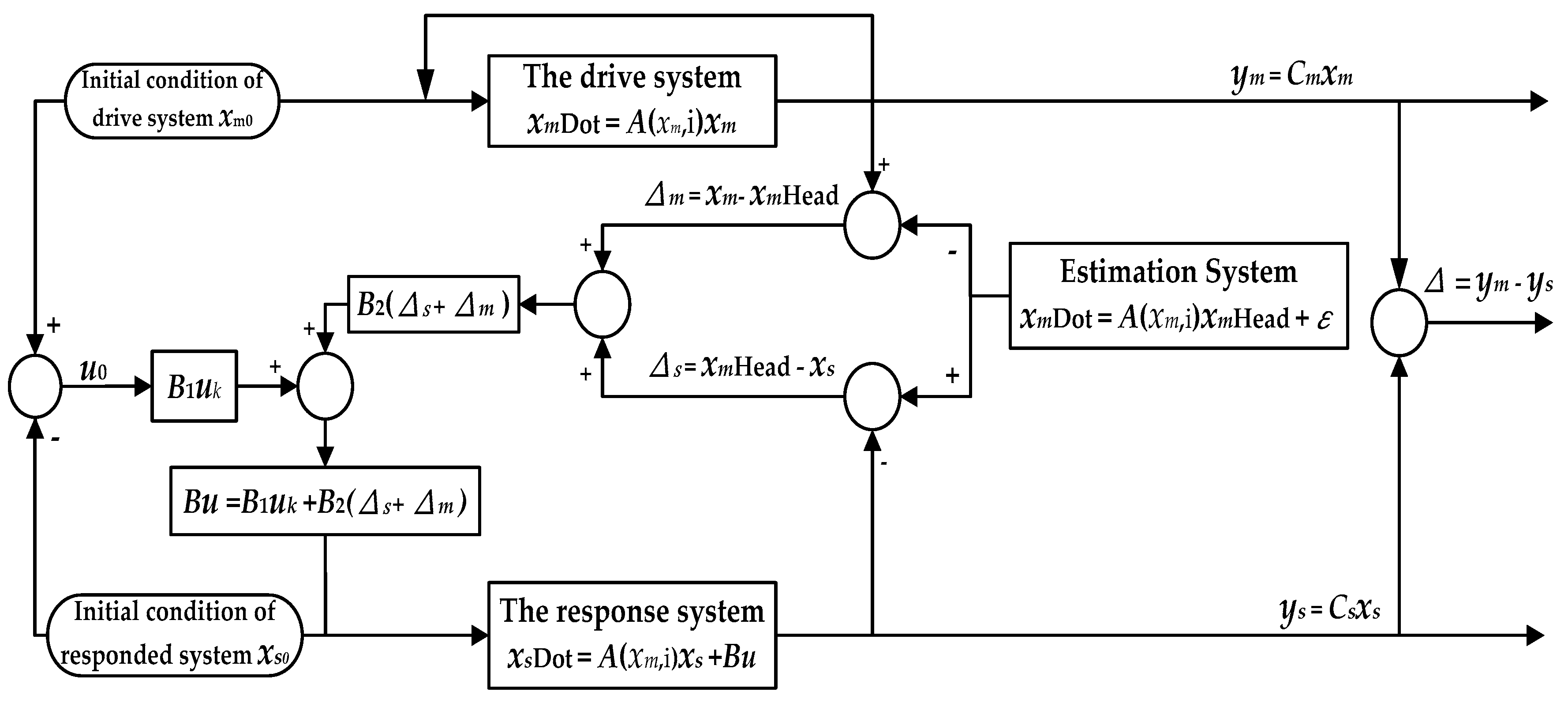
Figure 2.
The trajectories in two-dimensional x1, x3-space of systems.
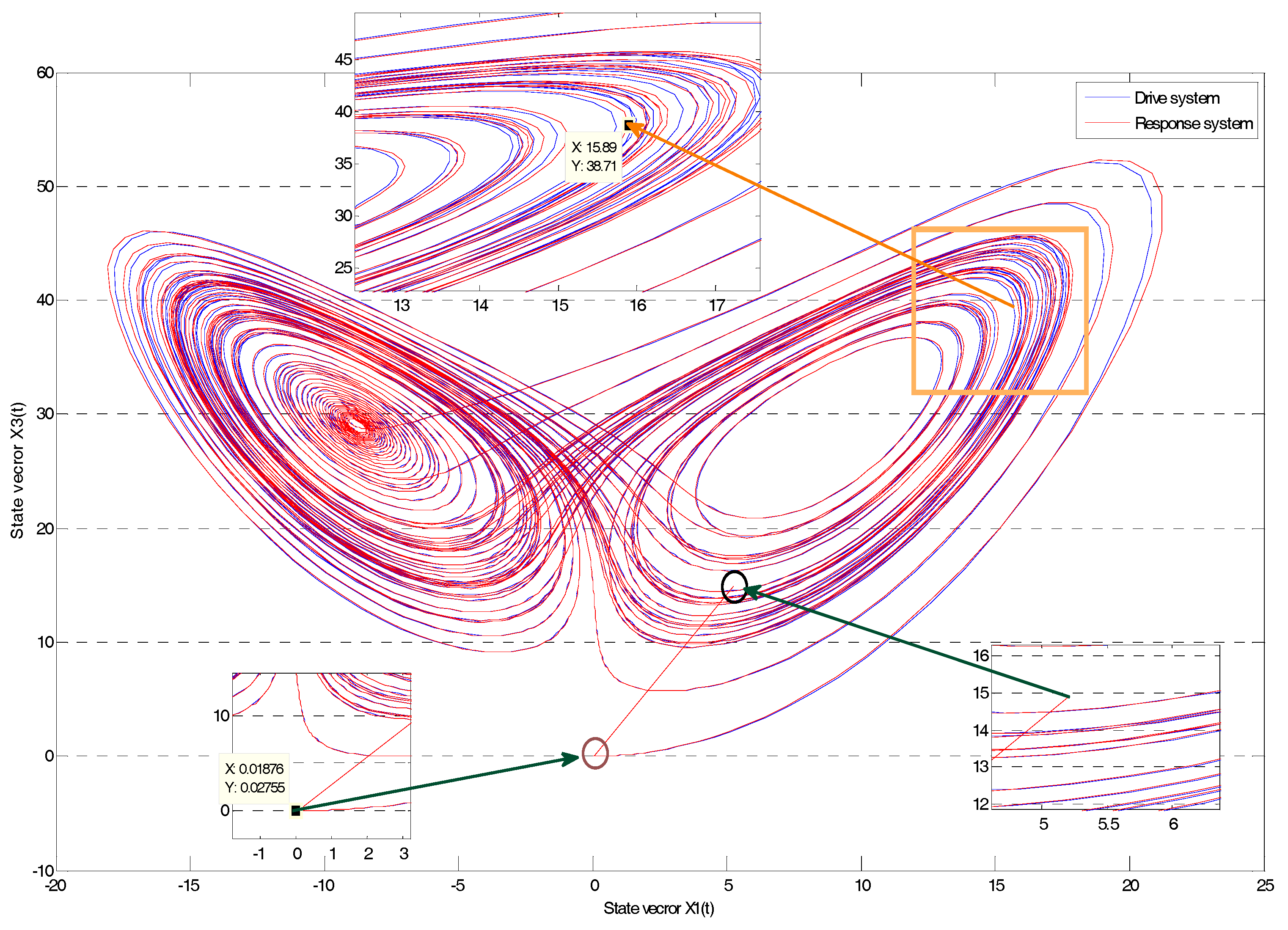
Figure 3.
The simulation of each component of the error dynamics system .
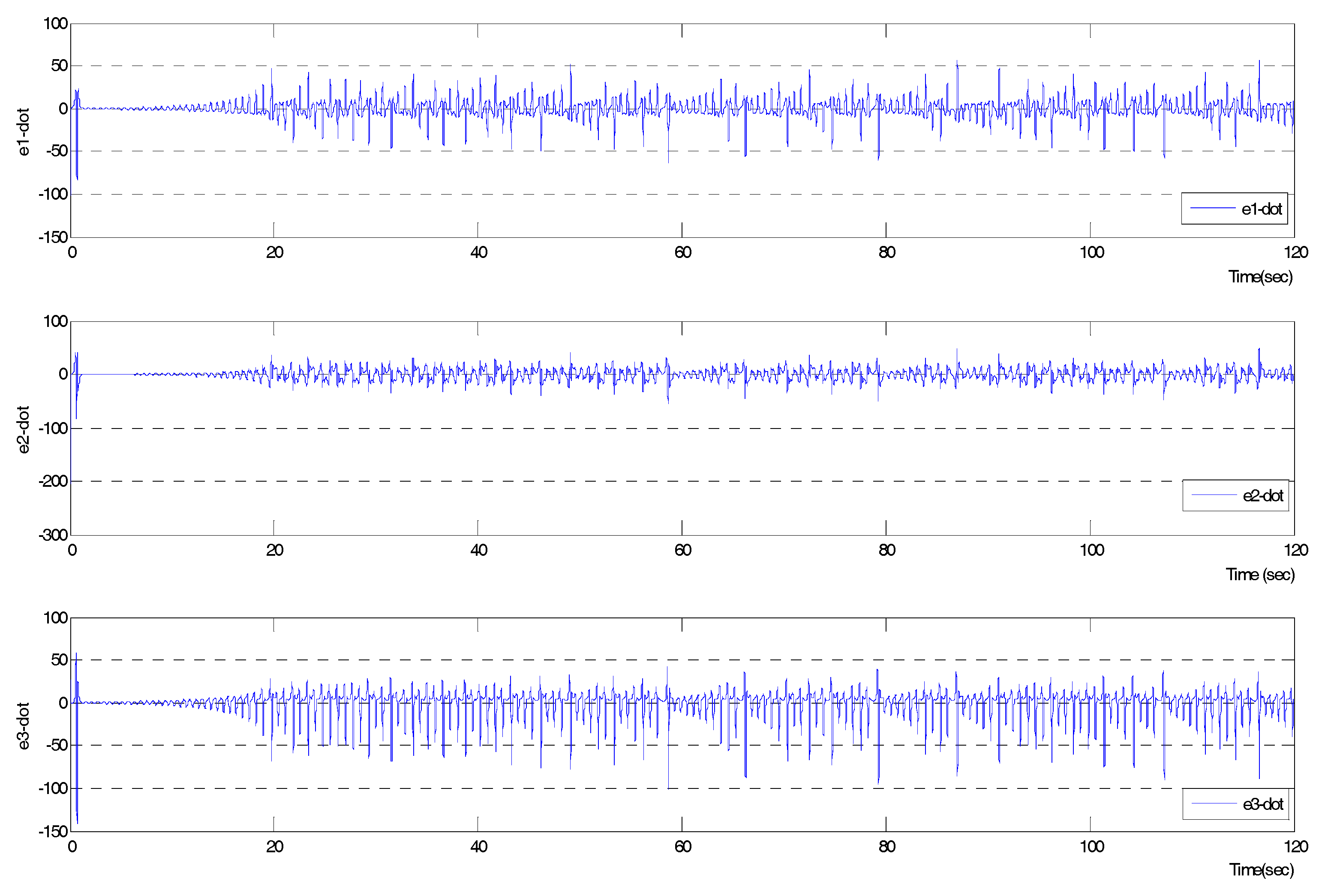
Figure 4.
The behavior of the iterative learning control law.

Figure 5.
The different behaviors of IL Care chosen as the worst learning law and listed as (a) B1 is identity matrix; and (b) B1 = Dig [0.1, 0.1, and 0.92].
Figure 5.
The different behaviors of IL Care chosen as the worst learning law and listed as (a) B1 is identity matrix; and (b) B1 = Dig [0.1, 0.1, and 0.92].

Figure 6.
The behavior of the derivative of the Lyapunov function (μ = 1).

Figure 7.
The behavior of the Iterative Learning Control operator and criterion.

Figure 8.
The synchronization error.


Table 1.
The Lyapunov function in different interval with different values of μ.
| Value of μ | [−1, 1] | (−∞, −1] | [1, ∞] | Total | Average |
|---|---|---|---|---|---|
| 1 | 1945 | 4811 | 5345 | 12001 | −2.5314 |
| 10 | 396 | 5473 | 6132 | 12001 | –19.896 |
| 50 | 93 | 5623 | 6285 | 12001 | –97.0546 |
| –10 | 393 | 6149 | 5459 | 12001 | 18.635 |
© 2018 by the authors. Licensee MDPI, Basel, Switzerland. This article is an open access article distributed under the terms and conditions of the Creative Commons Attribution (CC BY) license (http://creativecommons.org/licenses/by/4.0/).
Share and Cite
MDPI and ACS Style
Cheng, C.-K.; Chao, P.C.-P. Chaotic Synchronizing Systems with Zero Time Delay and Free Couple via Iterative Learning Control. Appl. Sci. 2018, 8, 177. https://doi.org/10.3390/app8020177
AMA Style
Cheng C-K, Chao PC-P. Chaotic Synchronizing Systems with Zero Time Delay and Free Couple via Iterative Learning Control. Applied Sciences. 2018; 8(2):177. https://doi.org/10.3390/app8020177
Chicago/Turabian StyleCheng, Chun-Kai, and Paul C. -P. Chao. 2018. "Chaotic Synchronizing Systems with Zero Time Delay and Free Couple via Iterative Learning Control" Applied Sciences 8, no. 2: 177. https://doi.org/10.3390/app8020177
Note that from the first issue of 2016, this journal uses article numbers instead of page numbers. See further details here.