An Examination of Thermal Features’ Relevance in the Task of Battery-Fault Detection

1
Centre ENET at VŠB-TU Ostrava, 708 00 Ostrava, Czech Republic
2
Department of Computer Science at VŠB-TU Ostrava, 708 00 Ostrava, Czech Republic
3
E.ON Distribuce, a.s., 370 01 České Budějovice, Czech Republic
*
Author to whom correspondence should be addressed.
Appl. Sci. 2018, 8(2), 182; https://doi.org/10.3390/app8020182
Submission received: 14 December 2017
/
Revised: 13 January 2018
/
Accepted: 22 January 2018
/
Published: 26 January 2018
(This article belongs to the Special Issue Novel Ideas for Infrared Thermography also Applied in Integrated Approaches)
Abstract
:Uninterruptible power supplies (UPS), represented by lead-acid batteries, play an important role in various kinds of industries. They protect industrial technologies from being damaged by dangerous interruptions of an electric power supply. Advanced UPS monitoring performed by a complex battery management system (BMS) prevents the UPS from sustaining more serious damage due to its timely and accurate battery-fault detection based on voltage metering. This technique is very advanced and precise but also very expensive on a long-term basis. This article describes an experiment applying infrared thermographic measurements during a long term monitoring and fault detection in UPS. The assumption that the battery overheat implies its damaged state is the leading factor of our experiments. They are based on real measured data on various UPS battery sets and several statistical examinations confirming the high relevancy of the thermal features with mostly over 90% detection accuracy. Such a model can be used as a supplement for lead-acid battery based UPS monitoring to ensure their higher reliability under significantly lower maintenance costs.
1. Introduction
A typical large scale uninterruptible power supply usually consists of a higher number of elementary batteries connected in series strings or series-parallel groups. Nowadays, most advanced uninterruptible power supplies (UPS) are equipped with a complex battery management system (BMS) in order to maintain their sustainable operability and prevent their degradation. The voltage of each battery is measured and the charging and discharging current of every battery in a string is controlled by balancers. This approach is necessary, especially for Li-ion batteries which are sensitive to overcharge and deep discharge [1].
In industrial purposed UPS, the lead-acid batteries are most frequently used due to their lower price and higher resistance to overcharge and deep discharge processes [2]. This implies a long payback period for any BMS application and most of the lead-acid based UPS are operated without battery management. Their charging process is controlled only by the measured battery voltage.
Modern BMS evaluates the condition and charge level of the batteries according to their voltage level, charging or discharging current and the cell temperature [3]. When the cell is damaged, overloaded or overcharged, it generates additional heat [4], which underlines the importance of temperature monitoring included as a part of the modern BMS. Temperature sensors must be placed directly on the cell surface, or inside the cell itself for proper functioning. In most applications, a simple thermistor is used for temperature monitoring. However, there are other types of sensors, developed especially for BMS purposes. Semiconductor CMOS sensors can provide high accuracy and linearity [4]. Flexible micro temperature sensors can be fabricated into the cells to provide high accuracy measurement with a short response time [5]. Temperature sensors may be also produced by a printed electronics technology [6], which can also positively affect their price. In special applications, an optical fiber can be used for the external and internal cell temperature monitoring [7]. This method is especially suitable in noisy environments.
In general, only contact sensors are being used for temperature monitoring of batteries. An infrared thermography, such as in studies of the thermal characteristics acquisitions [4] and factory diagnostics [5], was applied mostly for onsite inspections. Such an estimation of a battery condition according to its temperature leads to the overall difficulty and cost decrease while the performance remains the same or at least comparable.
Our article describes an experiment of the following parts:
- To gather an original dataset of charging and discharging lead-acid battery phases containing their voltage levels and temperatures that will be taken by an infrared thermography device placed above them.
- To extract valid features from the thermal images and to evaluate their clarity and relevance for a possible comparison.
- To demonstrate the relevance of the features by developing a fault detection model.
Such a study, according to the available literature, has been carried out for the first time and in case of success, it can lead to a design of an innovative and low cost BMS based on contact-less infrared thermography measurements.
This is usually done by a maintenance personnel. Goal of this paper is to describe the possibility of infrared thermography for long term monitoring and estimation of the condition of batteries in a string of UPS. Whole experiment was driven by the idea of creation of infrared thermography supplement to maintenance.
2. Experiment Design
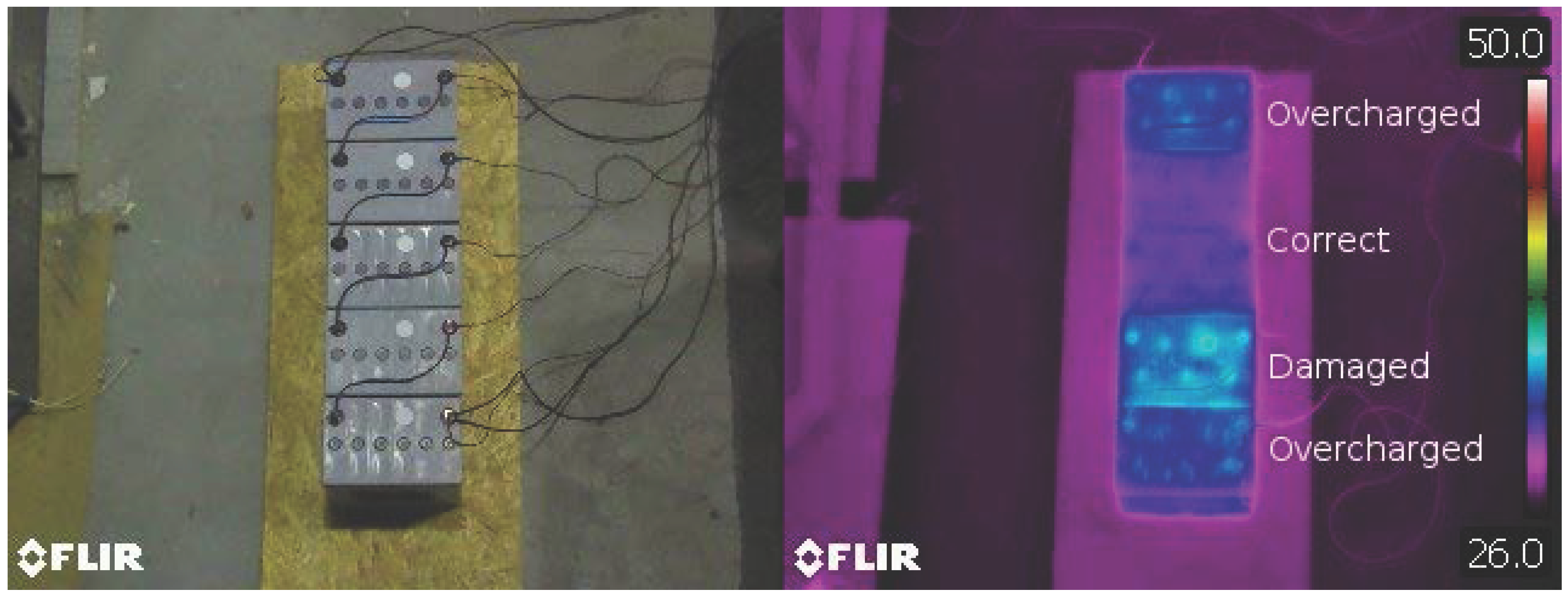
12 V/63 Ah lead-acid batteries were used in this experiment. First of all, high resolution thermograms were captured to discover significant temperature differences during battery malfunction. As presumed, a thermal map inhomogeneity is detectable in the battery with internal defects (Figure 1).
Having confirmed this, the experiment itself was conducted. Batteries were connected into the series string, containing from three to five batteries according to the experiment battery set. Before the experiment, all measured batteries were diagnosed for their current capacity (Table 1). Batteries with capacity below 50% were considered damaged.
An infrared camera was mounted on the ceiling of the laboratory for an automatic data acquisition with repetitive period of 1 min. The temperature range on the camera was set manually. The lower limit was set according to the ambient temperature and the upper limit according to the battery maximum allowed temperature. Value of the battery surface emissivity was estimated with the emissivity tape and set to 0.96. Voltage of each battery was measured with a data acquisition card with the same repetitive period as in thermogram acquisition (1 min). Batteries were mounted on a sheet of structural insulated panel which provided thermal insulation between the batteries and concrete floor in the laboratory (Figure 2).
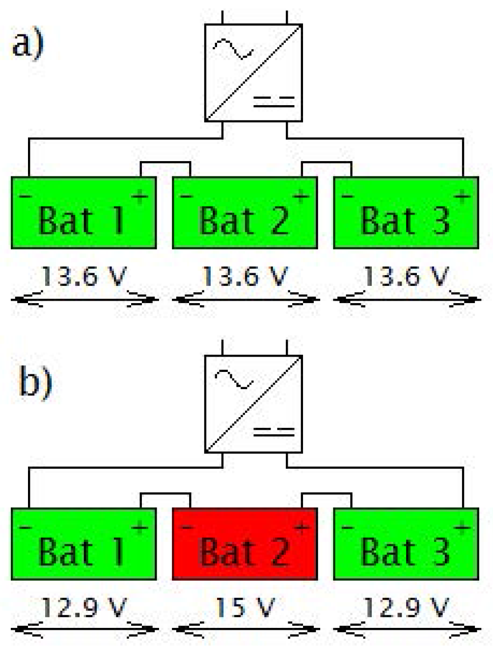
A voltage source was used as a charger. Its voltage was set according to the number of batteries in a battery set, multiplied by float charge voltage of the battery (13.6 V). This is the so-called constant voltage charging mode. Charging and discharging current was limited to 15 A to prevent the battery damage. Ideally, all the batteries in a series string have the same properties, which leads to a uniform distribution of voltage in each battery (Figure 3a). If one battery from the battery set is damaged, voltage distribution across the string is influenced by this malfunction. This failure leads to the overcharge or undercharge of the rest of batteries in the battery set (Figure 3b).
This is the reason why our experiment did not include any battery set containing only new batteries (with 100% capacity). A battery set containing only new batteries with nominal capacity has a uniform voltage distribution without any overcharging possibility.
Fault state of the battery was detected according to its voltage. If voltage of the battery overreached its maximum allowable value during the charging process (14.5 V), the battery state was labeled as fault. Similarly, when voltage of the battery dropped below the minimum allowable value (10.5 V) during discharging process, the battery state was also labeled as fault.
2.1. Thermal Image Processing
Relevant features from the thermal image need to be extracted in order to detect the battery overheat. The thermal image is a color image of pixels the values of which belong to RGB color space representing the temperature. Its exact level is based on a given scale defined by the camera adjustment (the scale is located on the right side of the thermal image in Figure 4 (left)). It may be seen that the scale consists of many color shades, and, unfortunately, the exact transform from the pixel color to the temperature level is not straightforward. The manufacturer provides an additional feature for temperature level estimation. Because our motivation is to keep the costs of the final device minimal, we attempted to develop our own temperature level estimation, which, for the sake of simplicity, was based on the assumption that the relation between pixel color and its temperature level is linear. On the other hand, this experiment does not require exactly precise estimations of the temperature levels and the slightly incorrect estimations will still expose the differences among the battery cells, which is still considered as relevant.
In recent years, several types of feature extraction approaches have been developed for thermal image processing in various fields of applications. The field of fault detection on electrical installation involved the maximum temperature difference between a hot spot and another point in its neighborhood [8]. Similarly, the combination of the spot temperature with the temperature difference of two similar components and the maximum admissible temperature of the component was used in [9,10], the difference of the maximum and the minimum temperatures in the object, and the surrounding area, respectively, was designed. In [11], the authors used statistical features computed making use the pixel intensities of the image regions. The considered features were the maximum, minimum, mean and the standard deviation of intensity level. The authors in [12] compared several features that can be extracted from thermal images, such as maximum region temperature, average region temperature, relative temperature difference between target and surrounding regions, or combinations of these features. The combination of those features was mostly considered the most relevant according to the presented results.
The transformation of a color-valued image matrix into a thermal-valued matrix assigns the temperature of the closest scale pixel to each transfered image pixel. The scale maximal () and minimal () temperatures are defined in the image (see Figure 4) and serve as the boundaries of normalization. The scale pixel values form an upwardly ordered vector where is the count of scale lines and their temperatures are estimated simply as . Consequently, each i-th image pixel obtains a temperature value of the most similar scale pixel as where the maximum similarity is considered the minimum distance d between two color-valued pixels, i.e. .
Inspired by the approaches mentioned above, we built our feature extraction aggregating the thermal image data. The absolute temperature of a selected spot does not necessary possess the information about the battery overheat as it may be affected by the ambient temperature that was computed as the average temperature of an area (white rectangle) next to the battery (see Figure 4 (right)). The overheat usually starts in one cell of a battery and then spreads to the entire battery. In order to detect overheat more precisely, we split the battery into several segments (see them visualized by the red lines in Figure 4 (right)) and the average temperature of each segment was computed. The number of segments per battery was set experimentally to 6. Finally, the ratios between the segment and ambient temperatures formed the thermal feature vector of the battery.
2.2. Methodology of Data Exploration
Raw vectors of the thermal and voltage features were processed in several ways to examine their distinguishing ability and relevance towards the fault indicating annotation. The following statistical methods were applied in our testing work-flow:
- Statistical analysis
- An estimation of correlation among temperature and voltage progress to test the similarity of their behavior.
- ANOVA test to examine the significance of statistical difference among battery sets
- Unsupervised clustering
- Dimensionality reduction of multivariate inputs on their intrinsic dimension with further clustering and its evaluation
- Supervised relevancy estimation
- Kraskov’s estimation of multivariate mutual information (MI) among reduced data and their annotations.
- k-nearest neighbor classification on four different sets of data (voltage and temperature inputs for predicting six battery sets and fault/failure-free battery set states respectively).
A brief description of the applied methods and algorithms follows.
2.2.1. Statistical Analysis
A correlation coefficient stands for the linear estimation of dependence between two random variables. The calculation is defined as their covariation divided by multiplication of their standard deviations (see Equation (1)) [13].
Result can vary between −1, 0 and 1, which stands for anti-correlation (the progress of variables possess opposite moves), no correlation (no statistical dependence between variables) and strong correlation (when variables have a similar progress) respectively.
Analysis of variance (ANOVA), developed by Ronald Fisher, is a set of tools aimed to test a variation in the means of several independent variables. The most important point in traditional ANOVA is a test of significance of the difference among the means of variables. This test permits us to conclude whether the differences among the means of several variables are too deviated to be attributed as a sampling error or a significant difference [14,15]. Based on that, the design of the adjusted hypothesis is defined as follows: , which means that under the zero hypothesis, there is no significant difference among the given means. The rejection of the zero-hypothesis will imply a presence of at least one variable with a significantly different mean from the rest of the variables. The additionally applied post-hoc analysis reveals which variable is the one with the confirmed difference.
2.2.2. Unsupervised Data Processing
Principal component analysis (PCA) is a linear transformation of matrix data, which reduces their dimension with regulated loss of information [16,17]. Such a process is achieved by embedding the original data into the linear subspace with a lower dimension in a way to preserve as much of relevant information as possible. It finds a mapping matrix M to lower the dimension with maximum variance, which is defined as a solution of an eigenproblem.
where is the covariance matrix of input data X. The mapping matrix M is orthogonal and is formed by principal components-eigenvectors of the covariance matrix . The matrix contains eigenvalues (the principal components) of the covariance matrix on diagonal. To provide the dimensionality reduction, the columns of the mapping matrix M are sorted according to the decreasing eigenvalues in the matrix . The mapping matrix is then truncated to keep only the first d principal components (the most significant components to keep the highest amount of information). A new data set Y reduced into the dimension d is then computed accordingly.
Principal Component Analysis was successfully applied in the area of feature extraction and signal processing [18], feature extraction [19] and it was also compared with other reduction techniques [20].
The cluster analysis is a grouping mechanism of samples into clusters according to their similarity that depends on a distance function and a given representation of the samples [21]. Such process was found helpful in various applications and, in our case, this process used to examine the relevancy of samples representation. The clear clusters with minimum overlap can imply lower noisiness and uncertainty, while the inseparable highly overlapped clusters imply the presence of irrelevant data representation.
The number of clusters can be determined by gap statistic [22]. It compares the total within intra-cluster variation for different values of k with their expected values under null reference distribution of the data. The estimate of the optimal clusters will be a value that maximizes the gap statistic (i.e., one that yields the largest gap statistic). This means that the clustering structure is far away from the random uniform distribution of points.
The Silhouette score may be calculated using the mean intra-cluster distance a and the mean nearest-cluster distance b for each sample [23] in order to evaluate the clarity of the solution. The Silhouette Coefficient of the solution is than . To be specific, b is the distance between a sample and the nearest cluster of which the sample is not a part.
2.2.3. Supervised Relevancy Estimation
The Kraskov algorithm is one of many approaches to estimate MI among two random variables. The Kraskov algorithm is widely used as it is considered as one of the most effective and accurate. It is able to evaluate the dependency among two multivariate variables in the same way as in case of univariate variables. Kraskov estimation is based on Kozachenko–Leonenko entropy estimation [24]:
where N means the number of samples in X, d is the dimensionality of samples x, means the volume of a d-dimensional unitary ball, and is twice the distance (usually chosen as the Euclidean distance) from to its k-th neighbor. The most known derivate of MI estimation has the following form (Equation (2)) [24]:
where is the number of points whose distance from is not greater than . As we can see, the Kraskov’s MI does not require the computation of underlying probability distributions of the given variables, but simply estimates the dependency by its neighbor based clustering, which simplifies the entire approach. A comparative review by Doquire and Verleysen confirmed its performance against other widely known estimation approaches [25].
K nearest neighbor (kNN) is a classification algorithm proposed by Cover and Hart [26]. It is a frequently used approach to classify future data due to its simplicity, ease of implementation and effectiveness. The model does not execute any training phase, only training tuples with their class labels are stored and the model performs the classification for each test instance. The class prediction of a given sample is simply estimated as a mean of its n neighbors, which implies that the process does not need any information about underlying data distribution. Several similarity functions can be employed in the process of neighbor searching, where the euclidean distance is one of the most used.
3. Adjustments, Testing and Results
The research of feature selection aims to estimate the dependency among various kinds of variables to select the most relevant subset from the entire dataset for the given classification or regression task [27,28]. The estimation of relevancy can vary with respect to the kind of variables on both sides, inputs or targets. In our case, the target variable is represented by the fault indicating annotation that varies between two states: 0–1 to distinguish fault and failure free battery sets, and 1–6 to distinguish between all examined battery sets (Table 1). The voltage and temperature vectors are applied as input variables and through all the executed tests, we are comparing whether the thermal features taken from the camera possess a relevancy comparable to the voltage data obtained directly from (dis)charged batteries. The voltage vectors are of length 3 or 5 which depends on the observed battery set. Similarly, temperature vectors lengths also vary among 96 or 160 (32 samples per battery). The ideal dataset, in case of classification, will possess a maximum correlation of all input variables towards the target one and minimal correlation among them (to avoid redundancies).
3.1. Statistical Testing
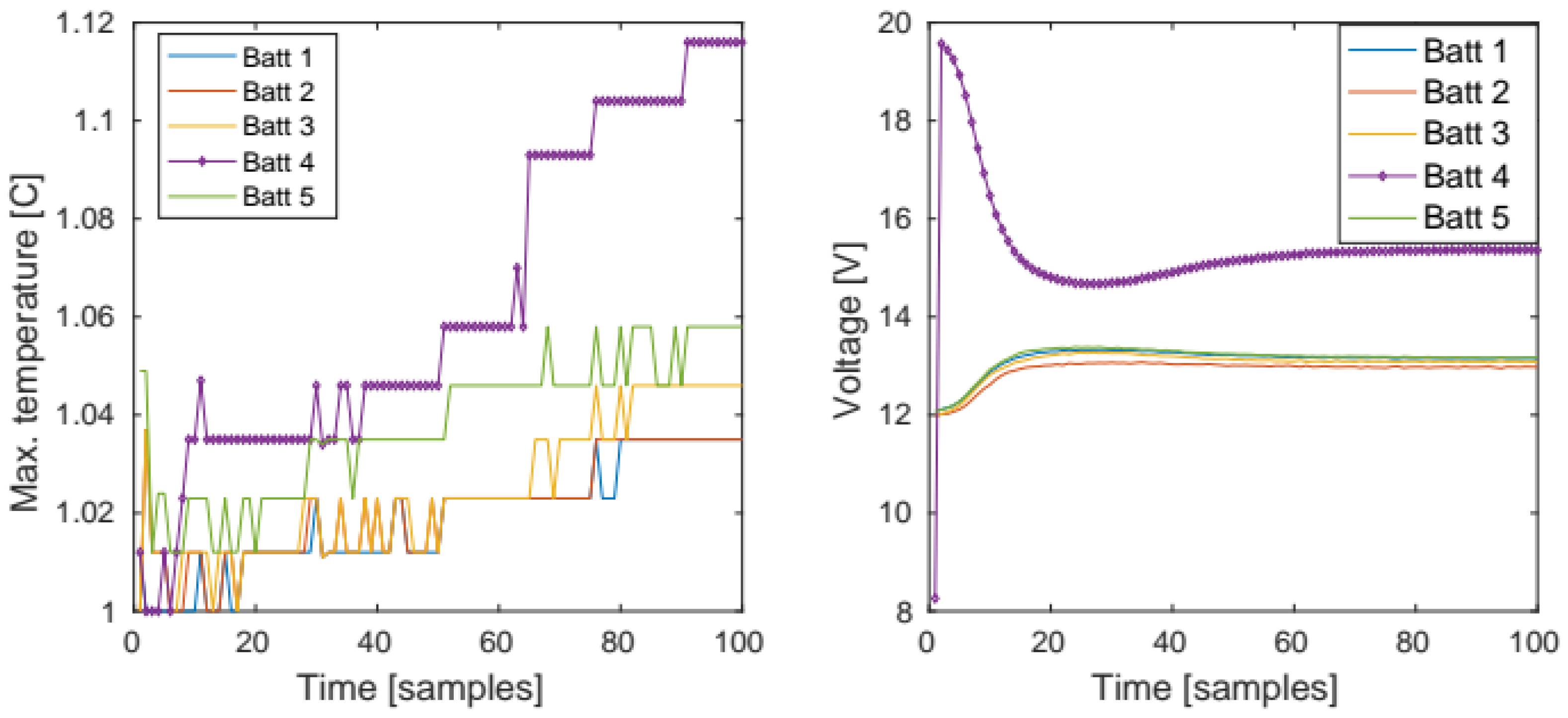
The correlation coefficient among multivariate variables or towards a categorical variable is not directly obtainable. What we can examine is the correlation between the obtained temperature and voltage data. The temperature of the battery is represented by six different time series, where each represents one measured surface spot. In case of fault, only some of them will increase their values, which will signify the battery overheat. The maximum values of these time series were therefore taken for the correlation estimation towards the voltage vector, because it is represented only by one time set and the battery malfunction is immediately readable from these data. In case of a high level of correlation, the implication about thermal features relevancy could arise. On the other hand, in case of uncorrelated behavior, we can only confirm no presence of redundancy among these variables, while relevance of the thermal data remains unconfirmed.
In Figure 5, we can see that the maximum temperature values and the voltage vectors do not possess similar behavior, which is also confirmed by their correlation coefficients. They are listed in Table 2 and their values were calculated on each battery of all battery sets and both (dis)charging processes.
For the following test, the raw data were transformed into time series of ranged values (the difference between the maximum and minimum value of the examined variables of the entire battery set during each measured time) in order to test the statistical difference of their values (ANOVA test). As it was mentioned previously, the result of ANOVA test is the rejection of null hypothesis, which states the statistical equality of means of the observed variables. In case the hypothesis is not rejected, it would be difficult to use variables without distinguishing ability.
In all cases, the resulting p-values dropped under the level of significance (: , : , : , : ), which implies the rejection of the null hypothesis in all cases. The graphical representation of ANOVA means comparison is depicted in Figure 6 and Figure 7.
Because the statistical difference among the groups of data was observed, we are allowed to perform an additional post-hoc analysis that will uncover which group significantly differs from others. The graphical representations of the post-hoc analysis results are depicted in Figure 8 and Figure 9. In case of the charging process, the battery sets 1 and 4 are clearly separable from the rest by both input variables, the temperature and the voltage range. These battery sets do not contain defected batteries, which is reflected by their smaller means of ranges.
3.2. Cluster Analysis
The following analysis will examine the quality of the data representation. The variables possess different sizes and during the following steps, we will aim to get the most relevant content from them. PCA is applied to modify the data and the clustering analysis can reveal how the quality of the data has changed.
In the following evaluations of clustering solutions, we will reduce the data dimension into its intrinsic dimension which was measured by likelihood estimation [29]. Data were reduced from their raw format (time set of measurements as rows × vector of measured features) into a dimensionally reduced matrix in order to unify the number of features (columns) and to lower the amount of redundancy and noise in the dataset. In cases of temperature data, the intrinsic dimension was always close to 5, therefore we reduced it into this dimension. We did not reduce the dimension of the voltage data, since it has already been measured in the dimension of 5 or 3 which reflected the number of batteries in the set. From now on, the temperature and voltage samples possess reduced vector sizes and are used as samples in cluster analysis and classification modeling.
Such data were clustered by k-means algorithm into several clustering solutions [30]. Each solution was defined by a different number of clusters. The quality of these solutions was examined by gap statistic that reveals which clustering solution is the most suitable for the given data and the silhouette score that evaluates the clarity of the solution. The results for charging and discharging process can be seen in Figure 10 and Figure 11.
3.3. Supervised Relevancy Estimation
The same representation of the examined variables is applied also in these final examinations. The Kraskov MI estimation simply calculates the amount of shared information between two variables. In all cases, it is the relevancy estimation of the multivariate input variable towards the target variable, which is represented by the binary output indicating only fault or failure-free state, or it is the categorical output variable containing identifiers of all examined battery sets. The value of MI is an entropy based measure that makes its output value relative to the character of examined data. A binary target variable possesses less sharable information, when compared to the target variable of continuous values, where the MI is not upper-bound.
Table 3 compares the values of estimated MI of both variables during charging and discharging processes. The Temp 1–6 means MI for thermal features towards the categorical variable containing the numbers of battery sets. The Temp 0–1 means MI for thermal features towards only the binary variable indicating a fault state. The MIs of the voltage vectors are depicted in the same manner accordingly.
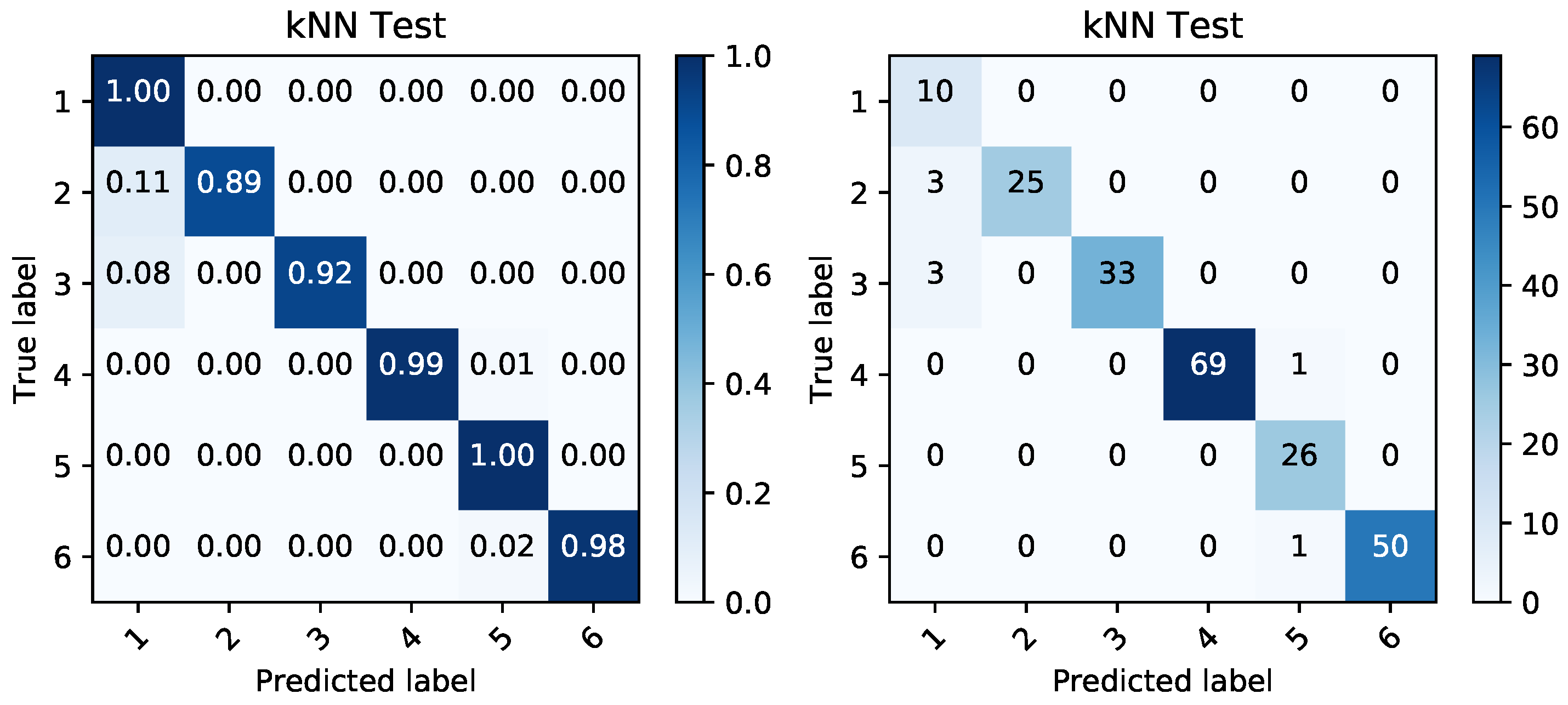
We employed the kNN classification algorithm and based on the given reduced representations, we modeled the classification performance of the randomly shuffled and split data. They were split into 60% for training data and 40% for testing data. The classification was again performed in order to classify the data into the binary targets and also to create a classification able to correctly distinguish between the given battery sets. The performance on this categorical target variable can be seen in Figure 12, Figure 13, Figure 14 and Figure 15. Simple percentages and absolute amounts of classification success rates are written on the diagonal of the confusion matrices, while the misclassified samples are spread in the rest of the matrix according to the distribution of the classification errors. For each confusion matrix, the predicted label stands for the predicted value of the given sample by trained kNN algorithm, while the true label is the desired value of that sample.
The quality of the classification is high. Table 4 shows the classification performance measures from the obtained binary classification. The accuracy (Equation (6)), precision (Equation (7)), recall (Equation (8)) and f-score (Equation (9)) were calculated from the predicted values of output variable [31] ( as true positive , true negative , false positive , and false negative ).
4. Discussion and Conclusions
The experiment presented in our article observes and measures a feature set describing the lead-acid batteries during their charging and discharging phases. Thermal and voltage based features were measured and examined for their relevance towards the battery-fault prediction. Several statistical tests revealed the facts about similarity of the features behavior, clarity and information content of the data representation and also the relevance towards the predicted battery state. The results of the correlation analysis between the maximum temperature values and obtained voltage levels are listed Table 2. These obtained coefficients mean that the most of the time, there is no correlation between these variables. This fact only confirms an absence of informational redundancy among the thermal and voltage data.
The analysis of variance (ANOVA) rejected the null hypothesis about the equality of the examined variables means. The results confirm that the examined input variables are significantly different among the tested battery sets and some of these sets are separable by the means of these variables.
The results of the cluster analysis visible in Figure 10 and Figure 11 demonstrate that 3 and 4 are the most suitable numbers of clusters according to the gap statistic. The clarity of the clusters is also the highest at these points as it is confirmed by silhouette score. Most of the time, this score value is over the value of 0.7, which implies a higher clarity of clusters, relevant data representation, and a lower amount of noise.
The final non-linear relevancy comparison was performed by Kraskov’s MI estimation. As we can see in Table 3, the relevancy of thermal features is very high and, in most cases, it is almost similar to the voltage data, which slightly confirms our hypothesis about thermal data applicability in the fault detection task. This small difference indicates the lower relevancy when compared to the very relevant voltage vectors. In our last test, we examined how much this difference affected the results of the classification algorithm, which was the simplest kNN in our case.
The kNN algorithm was used for multi-class classification and binary classification. In both cases, the input data from the thermal features were comparable to the voltage levels. The success rates above 80% in detection of most of the classes in case of thermal features confirm their validity of use. In all the multi-class detections, the voltage features perform better as it was expected.
In cases of binary-classification, the ability to predict whether the battery set contains a battery with malfunction, the voltage data were more relevant again. On the other hand, the thermal features relevance was very high and during the charing process, the difference was mostly lower than 2% only (see Table 4). This confirms the high relevancy of thermal data.
In conclusion, while the battery voltage features are certainly related to the predicted issue, their measurement requires an additional effort and cost. The execution of thermal measurements is less demanding, while its outcome preserves comparable relevance to the predicted issue according to the statistical tests performed in this study.
Although the time series of voltage and thermal features are not correlated, which is caused by different physical response times of measured features, they both possess relevant information for battery fault prediction. While the response time of the voltage feature is almost immediate and does not increase over time, the cell temperature can distinguish a defected cell after the heat appears on the surface. The image noise interference, lower quality of metering device, and imperfection involved by the assumption of linear relation between pixel value and a spot temperature could also play their roles in the decrease of relevance, which will be addressed in our future work. Further statistical tests were still able to confirm high clarity, valuable representation, and high relevance of the thermal data in the fault prediction task. Classification results proved the separability of thermal features in the multi-class and binary classification task. Thus, it is possible to create an infrared thermography monitoring system for battery fault detection able to replace the maintenance personnel.
The disadvantage of this method is the necessity of free space in the UPS surrounding area. The camera angle of view is another limiting factor; it is unsuitable for container-type UPS, but it can be easily applied in accumulator rooms, where sufficient distance between batteries and camera can be reached. In this case, such a monitoring system could provide almost the same results as voltage monitoring, but with a lower investment.
Acknowledgments
This work was supported by Project LO1404 ”Sustainable Development of Centre ENET”, VSB- Technical University of Ostrava and Grant Agency of the Czech Republic—TACR TH02020191 and VSB-TU internal grants SGS SP2018/58, SP2018/78 and SP2018/42.
Author Contributions
Stanislav Mišák is the author of the concept. Jan Fulneček and Jan Vaculík performed the experiment and data annotation. Michael Holuša processed the thermograms for the feature extraction and Tomáš Vantuch was responsible for design and execution of the statistical analysis.
Conflicts of Interest
The authors declare no conflict of interest.
References
- Andrea, D. Battery Management Systems for Large Lithium-Ion Battery Packs; Artech House: Norwood, MA, USA, 2010. [Google Scholar]
- Crompton, T.P. Battery Reference Book; Newnes: Oxford, UK, 2000. [Google Scholar]
- Li, J. Advances in Battery Manufacturing, Service, and Management Systems; John Wiley & Sons: Hoboken, NJ, USA, 2016. [Google Scholar]
- Pesaran, A.A.; Keyser, M. Thermal characteristics of selected EV and HEV batteries. In Proceedings of the Sixteenth Annual Battery Conference on Applications and Advances, Long Beach, CA, USA, 12 January 2001; pp. 219–225. [Google Scholar]
- Robinson, J.B.; Engebretsen, E.; Finegan, D.P.; Darr, J.; Hinds, G.; Shearing, P.R.; Brett, D.J. Detection of Internal Defects in Lithium-Ion Batteries Using Lock-in Thermography. ECS Electrochem. Lett. 2015, 4, A106–A109. [Google Scholar] [CrossRef]
- Grosch, J.; Teuber, E.; Jank, M.; Lorentz, V.; März, M.; Frey, L. Device optimization and application study of low cost printed temperature sensor for mobile and stationary battery based Energy Storage Systems. In Proceedings of the 2015 IEEE International Conference on Smart Energy Grid Engineering (SEGE), Oshawa, ON, Canada, 17–19 August 2015; pp. 1–7. [Google Scholar]
- Novais, S.; Nascimento, M.; Grande, L.; Domingues, M.F.; Antunes, P.; Alberto, N.; Leitão, C.; Oliveira, R.; Koch, S.; Kim, G.T.; et al. Internal and external temperature monitoring of a Li-ion battery with Fiber Bragg grating sensors. Sensors 2016, 16, 1394. [Google Scholar] [CrossRef] [PubMed]
- Chou, Y.C.; Yao, L. Automatic diagnostic system of electrical equipment using infrared thermography. In Proceedings of the SOCPAR’09 International Conference of Soft Computing and Pattern Recognition, Malacca, Malaysia, 4–7 December 2009; pp. 155–160. [Google Scholar]
- Prazzo, C.E.; Antunes, M.; Turra, A.; Pereira, J. The use of fuzzy logic to classify heating severity of components applied in a thermography based maintenance. In Proceedings of the XVIII Congresso Brasileiro de Automática, Bonito, Brazil, 13–16 September 2010; Volume 12. [Google Scholar]
- Lu, J.; Zhao, C.; Jiang, Z.; Guan, S.; Qian, Y.; Xia, D. Research of infrared thermal on-line detection technology of zero resistance insulator. In Proceedings of the Cross Strait Quad-Regional Radio Science and Wireless Technology Conference (CSQRWC), Harbin, China, 26–30 July 2011; Volume 2, pp. 1390–1393. [Google Scholar]
- Ahmed, M.M.; Huda, A.; Isa, N.A.M. Recursive construction of output-context fuzzy systems for the condition monitoring of electrical hotspots based on infrared thermography. Eng. Appl. Artif. Intell. 2015, 39, 120–131. [Google Scholar] [CrossRef]
- Jadin, M.S.; Taib, S.; Ghazali, K.H. Feature extraction and classification for detecting the thermal faults in electrical installations. Measurement 2014, 57, 15–24. [Google Scholar] [CrossRef]
- Sedgwick, P. Pearson’s correlation coefficient. BMJ 2012, 345. [Google Scholar] [CrossRef]
- Hocking, R.R. Methods and Applications of Linear Models: Regression and the Analysis of Variance; John Wiley & Sons: Hoboken, NJ, USA, 2013. [Google Scholar]
- Larson, M.G. Analysis of variance. Circulation 2008, 117, 115–121. [Google Scholar] [CrossRef] [PubMed]
- Wold, S.; Esbensen, K.; Geladi, P. Principal component analysis. Chemom. Intell. Lab. Syst. 1987, 2, 37–52. [Google Scholar] [CrossRef]
- Partridge, M.; Calvo, R.A. Fast dimensionality reduction and simple PCA. Intell. Data Anal. 1998, 2, 203–214. [Google Scholar] [CrossRef]
- Sorzano, C.O.S.; Vargas, J.; Montano, A.P. A survey of dimensionality reduction techniques. arXiv, 2014; arXiv:1403.2877. [Google Scholar]
- Kim, K.I.; Jung, K.; Kim, H.J. Face recognition using kernel principal component analysis. IEEE Signal Process. Lett. 2002, 9, 40–42. [Google Scholar]
- Vantuch, T.; Snasel, V.; Zelinka, I. Dimensionality Reduction Method’s Comparison Based on Statistical Dependencies. Procedia Comput. Sci. 2016, 83, 1025–1031. [Google Scholar] [CrossRef]
- Kaufman, L.; Rousseeuw, P.J. Finding Groups in Data: An Introduction to Cluster Analysis; John Wiley & Sons: Hoboken, NJ, USA, 2009; Volume 344. [Google Scholar]
- Tibshirani, R.; Walther, G.; Hastie, T. Estimating the number of clusters in a data set via the gap statistic. J. R. Stat. Soc. Ser. B Stat. Methodol. 2001, 63, 411–423. [Google Scholar] [CrossRef]
- Rousseeuw, P.J. Silhouettes: A graphical aid to the interpretation and validation of cluster analysis. J. Comput. Appl. Math. 1987, 20, 53–65. [Google Scholar] [CrossRef]
- Kraskov, A.; Stögbauer, H.; Grassberger, P. Estimating mutual information. Phys. Rev. E 2004, 69, 066138. [Google Scholar] [CrossRef] [PubMed]
- Doquire, G.; Verleysen, M. A Comparison of Multivariate Mutual Information Estimators for Feature Selection. In Proceedings of the ICPRAM 2012 Vilamoura, Algarve, Portugal, 6–8 February 2012; pp. 176–185. [Google Scholar]
- Cover, T.; Hart, P. Nearest neighbor pattern classification. IEEE Trans. Inf. Theory 1967, 13, 21–27. [Google Scholar] [CrossRef]
- Guyon, I.; Elisseeff, A. An introduction to variable and feature selection. J. Mach. Learn. Res. 2003, 3, 1157–1182. [Google Scholar]
- Kira, K.; Rendell, L.A. The feature selection problem: Traditional methods and a new algorithm. In Proceedings of the AAAI’92 Proceedings of the Tenth National Conference on Artificial Intelligence, San Jose, CA, USA, 12–16 July 1992; Volume 2, pp. 129–134. [Google Scholar]
- Levina, E.; Bickel, P.J. Maximum likelihood estimation of intrinsic dimension. In Advances in Neural Information Processing Systems; The MIT Press: Cambridge, MA, USA, 2005; pp. 777–784. [Google Scholar]
- Hartigan, J.A.; Wong, M.A. Algorithm AS 136: A k-means clustering algorithm. J. R. Stat. Soc. Ser. C Appl. Stat. 1979, 28, 100–108. [Google Scholar] [CrossRef]
- Powers, D.M. Evaluation: From precision, recall and F-measure to ROC, informedness, markedness and correlation. J. Mach. Learn. Technol. 2011, 2, 37–63. [Google Scholar]
Figure 1.
Thermogram of damaged and undamaged battery.
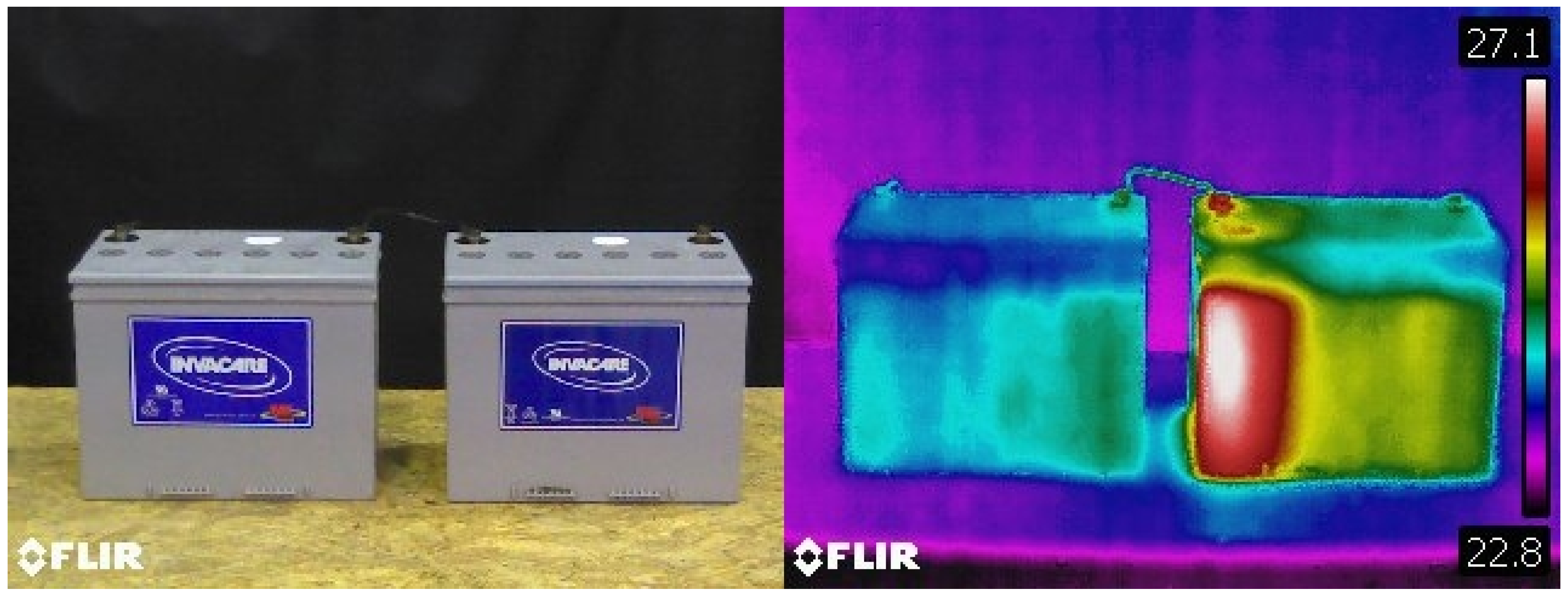
Figure 2.
Thermogram of damaged and undamaged battery.

Figure 3.
Voltage distribution in battery set during constant voltage charging. (a) represents the battery set without any damaged battery-voltage levels are equally distributed, while in (b) the battery set contains one damaged battery where the voltage level is increased.
Figure 3.
Voltage distribution in battery set during constant voltage charging. (a) represents the battery set without any damaged battery-voltage levels are equally distributed, while in (b) the battery set contains one damaged battery where the voltage level is increased.

Figure 4.
The input thermal image in RGB space (left); the image transformed to the temperature space (center); and the the image with highlighted areas of batteries (green), battery segments (red), and battery surroundings (white) (right).
Figure 4.
The input thermal image in RGB space (left); the image transformed to the temperature space (center); and the the image with highlighted areas of batteries (green), battery segments (red), and battery surroundings (white) (right).
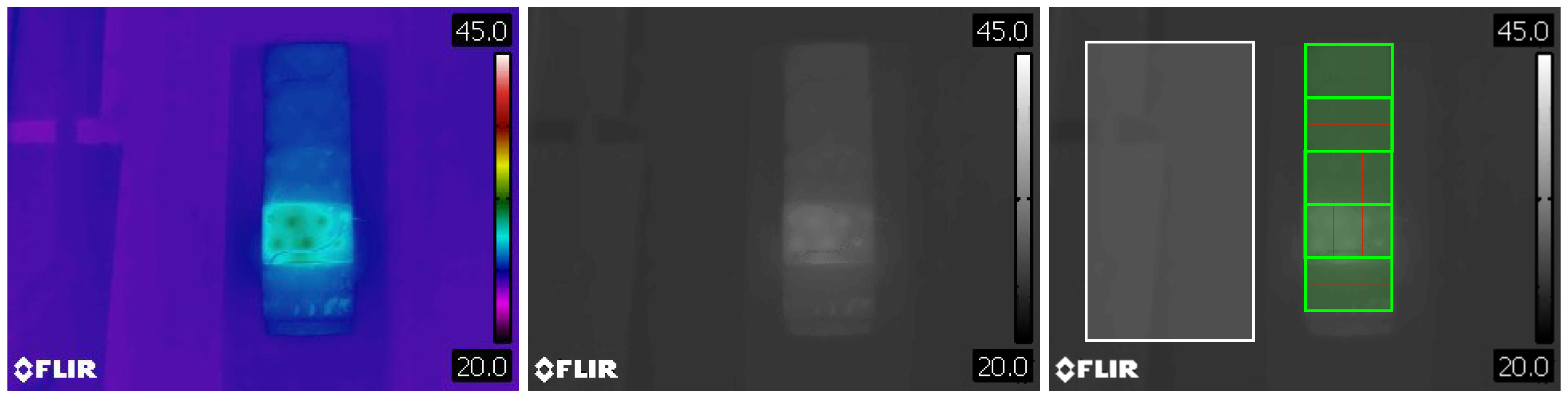
Figure 5.
The maximum measured values on the given battery set at the given time. The temperature data are visualized on the left side and the voltage data on the right side.
Figure 5.
The maximum measured values on the given battery set at the given time. The temperature data are visualized on the left side and the voltage data on the right side.

Figure 6.
The analysis of variance of temperature (left) and voltage (right) ranges during the charging period.
Figure 6.
The analysis of variance of temperature (left) and voltage (right) ranges during the charging period.
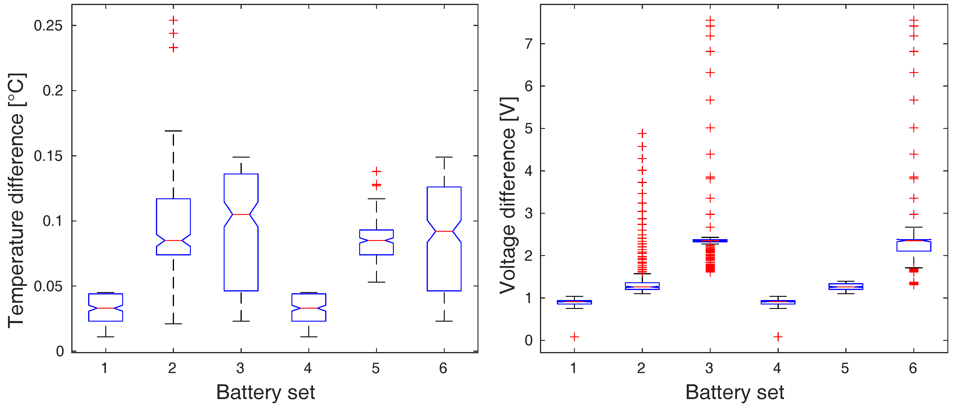
Figure 7.
The analysis of variance of temperature (left) and voltage (right) ranges during discharging period.
Figure 7.
The analysis of variance of temperature (left) and voltage (right) ranges during discharging period.
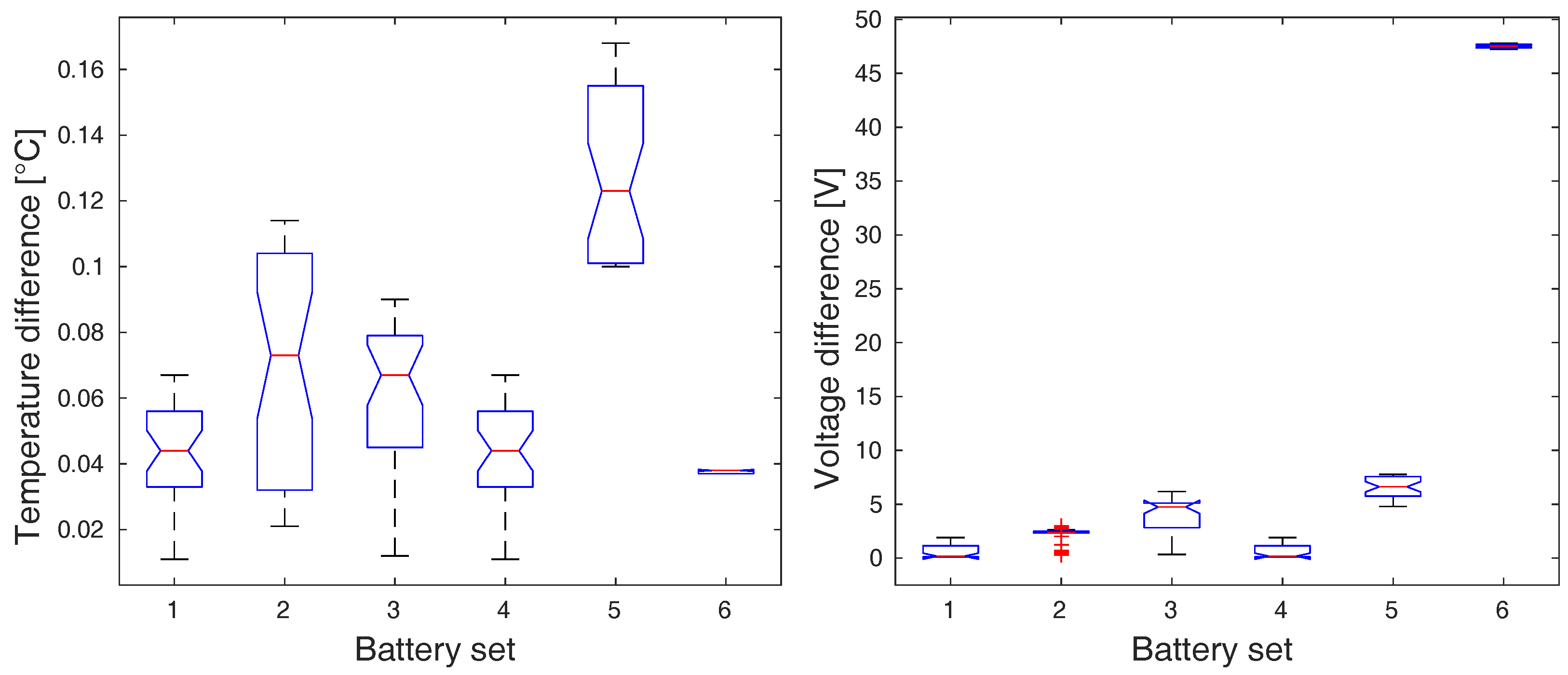
Figure 8.
The post-hoc analysis of means of temperature (left) and voltage (right) ranges during charging period.
Figure 8.
The post-hoc analysis of means of temperature (left) and voltage (right) ranges during charging period.
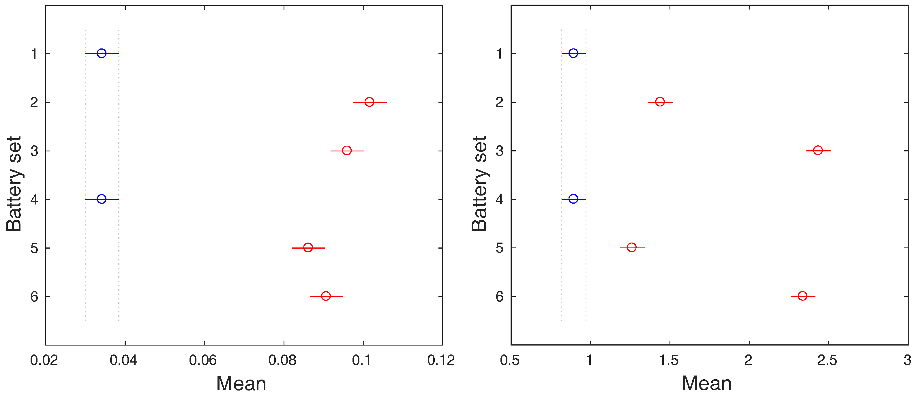
Figure 9.
The post-hoc analysis of means of temperature (left) and voltage (right) ranges during discharging period.
Figure 9.
The post-hoc analysis of means of temperature (left) and voltage (right) ranges during discharging period.
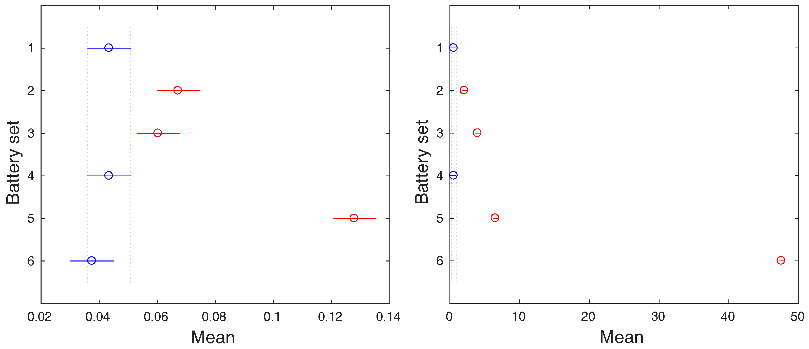
Figure 10.
The gap statistic (left) and the silhouette score (right) of the obtained clustering solutions of reduced data that are measured during charging period.
Figure 10.
The gap statistic (left) and the silhouette score (right) of the obtained clustering solutions of reduced data that are measured during charging period.
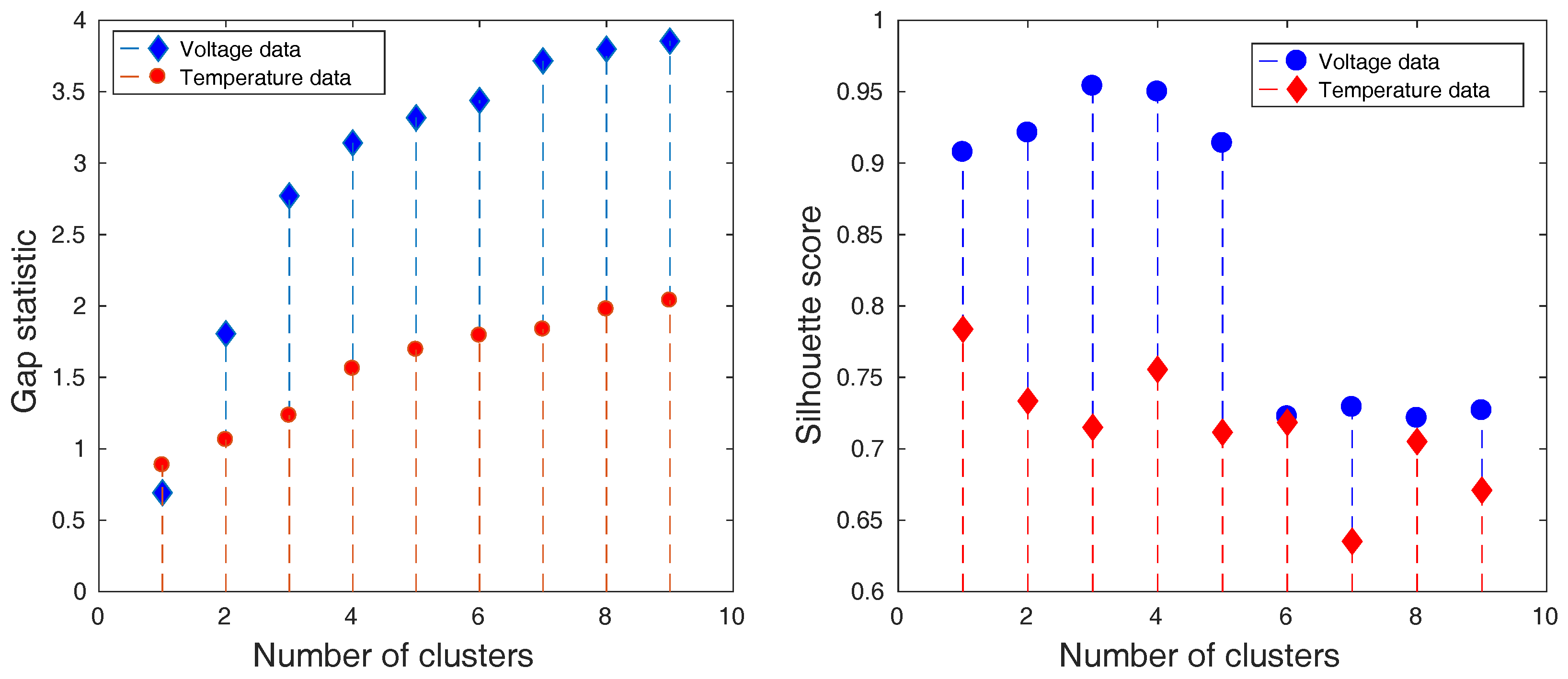
Figure 11.
The gap statistic (left) and the silhouette score (right) of the obtained clustering solutions of reduced data that are measured during discharging period.
Figure 11.
The gap statistic (left) and the silhouette score (right) of the obtained clustering solutions of reduced data that are measured during discharging period.
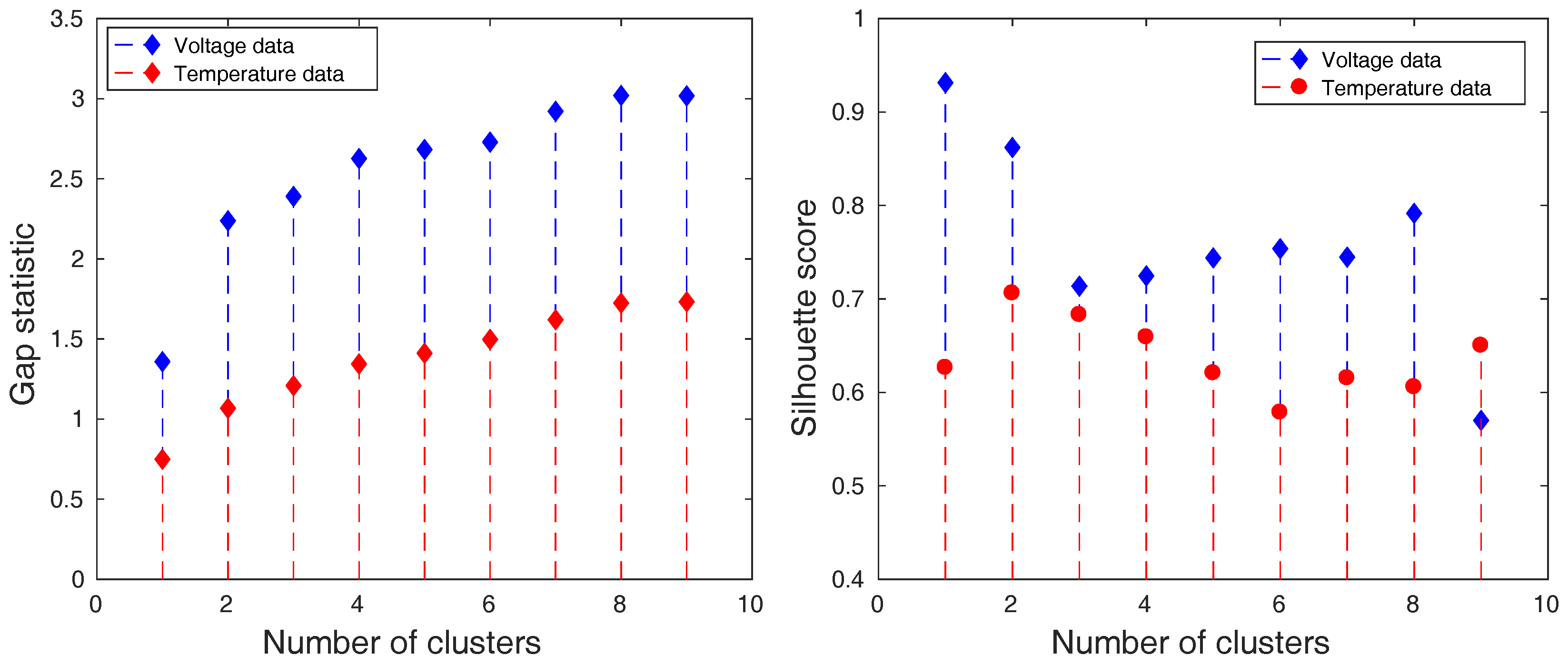
Figure 12.
Confusion matrices produced by kNN prediction based on temperature data during charging period. The matrix of percentages between correctly and incorrectly classified samples (left) is accompanied by a confusion matrix covering the absolute values of the same classified samples (right).
Figure 12.
Confusion matrices produced by kNN prediction based on temperature data during charging period. The matrix of percentages between correctly and incorrectly classified samples (left) is accompanied by a confusion matrix covering the absolute values of the same classified samples (right).
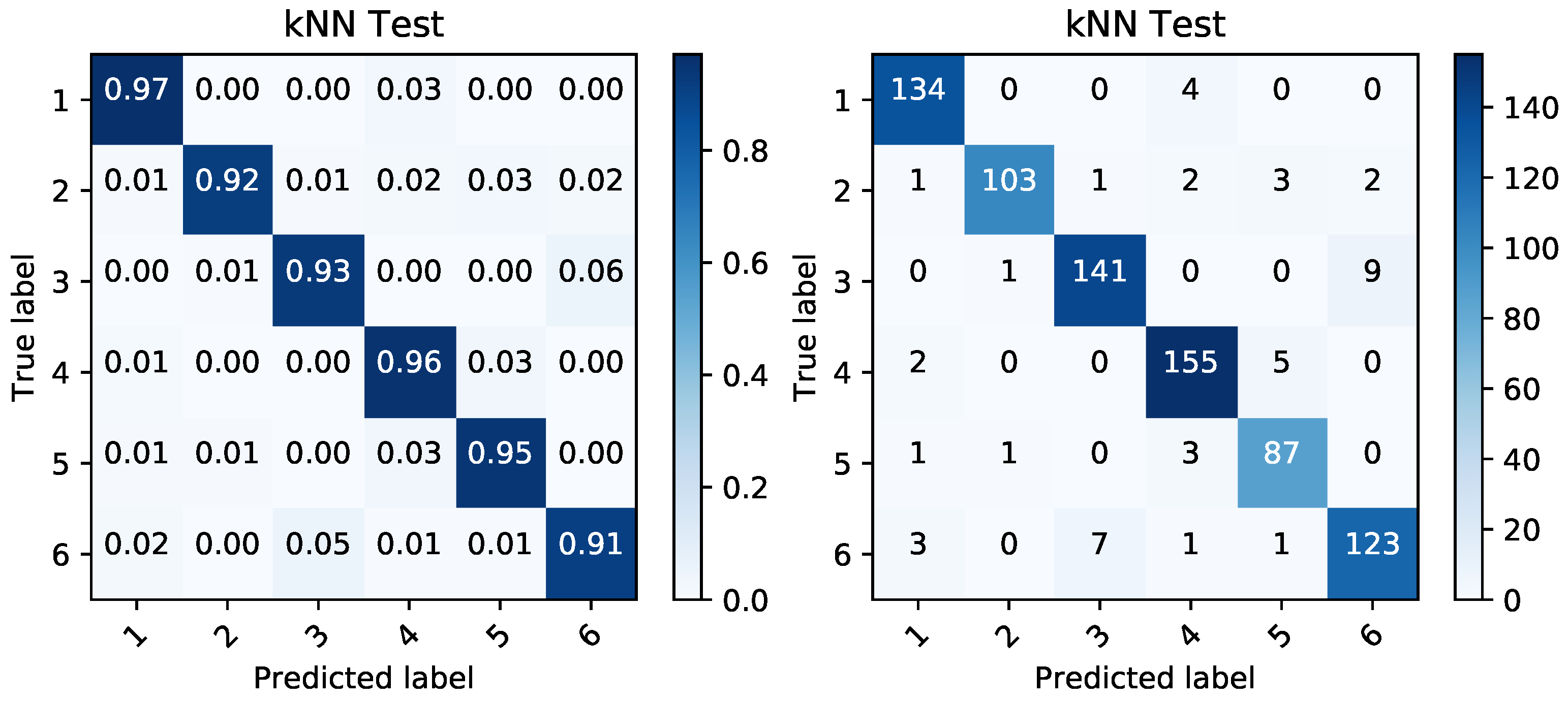
Figure 13.
Confusion matrices produced by k nearest neighbor (kNN) prediction based on voltage data during charging period. The matrix of percentages between correctly and incorrectly classified samples (left) is accompanied by a confusion matrix covering the absolute values of the same classified samples (right).
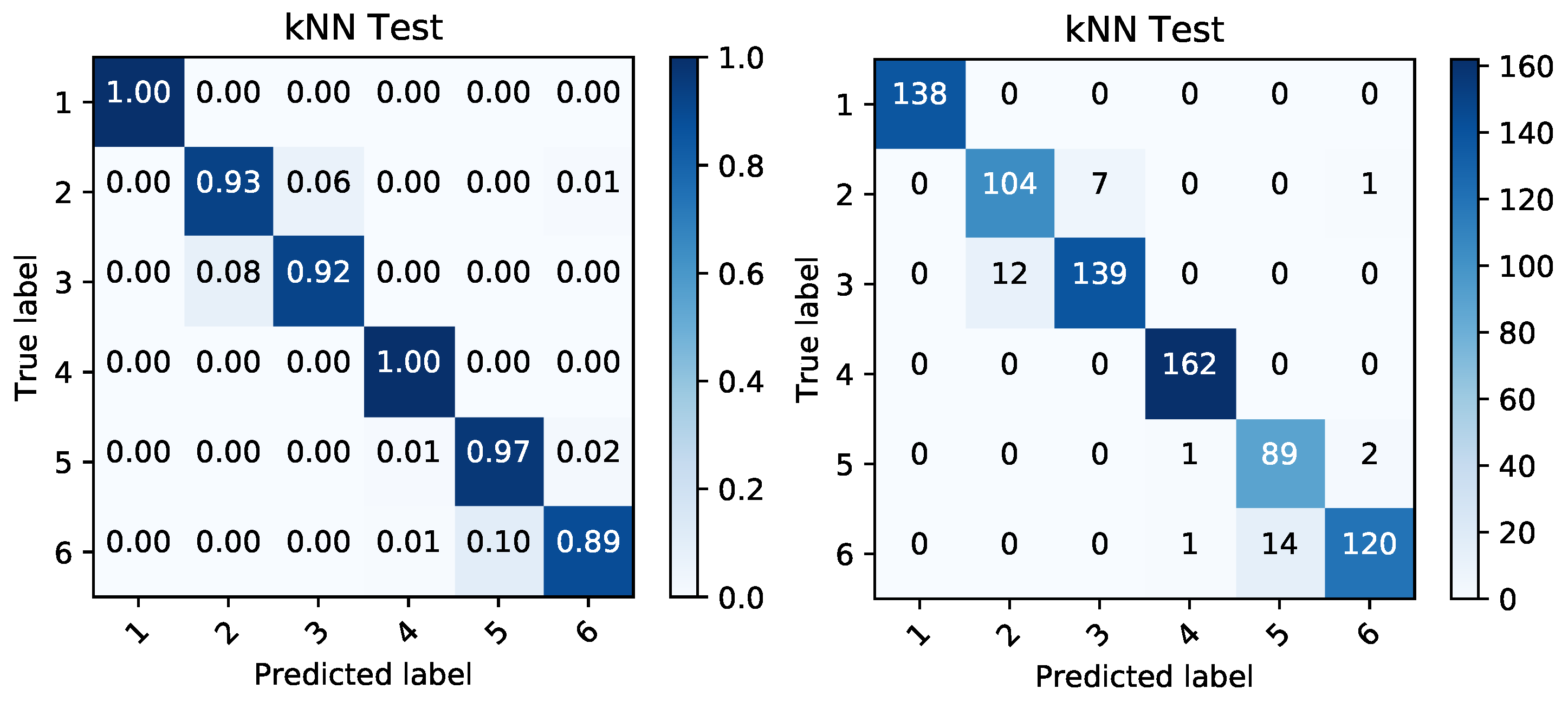
Figure 14.
Confusion matrices produced by kNN prediction based on temperature data during discharging period. The matrix of percentages between correctly and incorrectly classified samples (left) is accompanied by a confusion matrix covering the absolute values of the same classified samples (right).
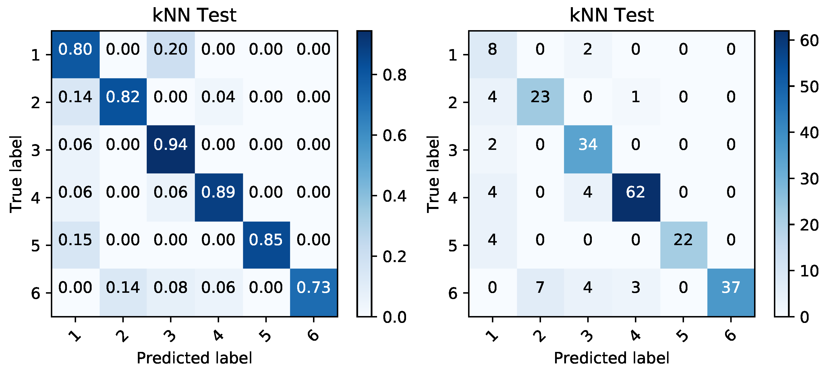
Figure 15.
Confusion matrices produced by kNN prediction based on voltage data during discharging period. The matrix of percentages between correctly and incorrectly classified samples (left) is accompanied by a confusion matrix covering the absolute values of the same classified samples (right).
Figure 15.
Confusion matrices produced by kNN prediction based on voltage data during discharging period. The matrix of percentages between correctly and incorrectly classified samples (left) is accompanied by a confusion matrix covering the absolute values of the same classified samples (right).

Table 1.
Percentage values of battery actual capacity (from nominal value).
| (%) | Battery Set | |||||
|---|---|---|---|---|---|---|
| 1 | 2 | 3 | 4 | 5 | 6 | |
| Battery 1 | 67 | 67 | 67 | 67 | 67 | 67 |
| Battery 2 | 76 | 76 | 76 | 76 | 76 | 22 |
| Battery 3 | 76 | 76 | 76 | 76 | 25 | 25 |
| Battery 4 | 53 | 22 | 24 | - | - | - |
| Battery 5 | 65 | 65 | 65 | - | - | - |
Table 2.
Correlation coefficients between pairs of variables (thermal range and voltage range) of all battery sets during both processes (charging and discharging).
Table 2.
Correlation coefficients between pairs of variables (thermal range and voltage range) of all battery sets during both processes (charging and discharging).
| Charging | Discharging | Charging | Discharging | ||||
|---|---|---|---|---|---|---|---|
| BS1 | Batt1 | −0.429 | −0.691 | BS4 | Batt1 | 0.403 | −0.213 |
| Batt2 | −0.278 | −0.749 | Batt2 | 0.498 | −0.548 | ||
| Batt3 | −0.094 | −0.787 | Batt3 | −0.014 | −0.171 | ||
| Batt4 | 0.322 | −0.634 | |||||
| Batt5 | −0.074 | −0.615 | |||||
| BS2 | Batt1 | 0.665 | −0.482 | BS5 | Batt1 | 0.577 | −0.809 |
| Batt2 | 0.255 | −0.639 | Batt2 | 0.65 | −0.887 | ||
| Batt3 | 0.262 | −0.905 | Batt3 | −0.228 | −0.091 | ||
| Batt4 | 0.387 | −0.654 | |||||
| Batt5 | 0.672 | −0.835 | |||||
| BS3 | Batt1 | 0.297 | −0.73 | BS6 | Batt1 | −0.609 | −0.58 |
| Batt2 | 0.408 | −0.653 | Batt2 | −0.631 | −0.76 | ||
| Batt3 | 0.144 | −0.897 | Batt3 | 0.856 | −0.337 | ||
| Batt4 | −0.11 | −0.915 | |||||
| Batt5 | 0.097 | −0.821 |
Table 3.
The MI coefficients from multivariate estimation gathered from reduced thermal and voltage vectors during charging and discharging period.
Table 3.
The MI coefficients from multivariate estimation gathered from reduced thermal and voltage vectors during charging and discharging period.
| Kraskov’s MI | Temp 1–6 | Temp 0–1 | Volt 1–6 | Volt 0–1 |
|---|---|---|---|---|
| Charging | 1.6599 | 0.6552 | 1.6880 | 0.6561 |
| Discharging | 1.4259 | 0.5324 | 1.6182 | 0.5992 |
Table 4.
Evaluations of binary classification performance (fault and failure-free battery battery set) processed on dimensionally reduced data obtained from charging and discharging process.
Table 4.
Evaluations of binary classification performance (fault and failure-free battery battery set) processed on dimensionally reduced data obtained from charging and discharging process.
| Charging | Temp Data | Voltage Data |
|---|---|---|
| Accuracy (%) | 97.72 | 99.75 |
| Precision (%) | 99.16 | 100 |
| Recall (%) | 97.13 | 99.59 |
| F-score (%) | 98.14 | 99.79 |
| Discharging | Temp Data | Voltage Data |
| Accuracy (%) | 90.95 | 97.74 |
| Precision (%) | 96.21 | 100 |
| Recall (%) | 89.44 | 96.48 |
| F-score (%) | 92.70 | 98.21 |
© 2018 by the authors. Licensee MDPI, Basel, Switzerland. This article is an open access article distributed under the terms and conditions of the Creative Commons Attribution (CC BY) license (http://creativecommons.org/licenses/by/4.0/).
Share and Cite
MDPI and ACS Style
Vantuch, T.; Fulneček, J.; Holuša, M.; Mišák, S.; Vaculík, J. An Examination of Thermal Features’ Relevance in the Task of Battery-Fault Detection. Appl. Sci. 2018, 8, 182. https://doi.org/10.3390/app8020182
AMA Style
Vantuch T, Fulneček J, Holuša M, Mišák S, Vaculík J. An Examination of Thermal Features’ Relevance in the Task of Battery-Fault Detection. Applied Sciences. 2018; 8(2):182. https://doi.org/10.3390/app8020182
Chicago/Turabian StyleVantuch, Tomáš, Jan Fulneček, Michael Holuša, Stanislav Mišák, and Jan Vaculík. 2018. "An Examination of Thermal Features’ Relevance in the Task of Battery-Fault Detection" Applied Sciences 8, no. 2: 182. https://doi.org/10.3390/app8020182
Note that from the first issue of 2016, this journal uses article numbers instead of page numbers. See further details here.