Article

Wind Power Forecasting Using Multi-Objective Evolutionary Algorithms for Wavelet Neural Network-Optimized Prediction Intervals

Key Laboratory of Advanced Process Control for Light Industry, Jiangnan University, Wuxi 214122, China
*
Author to whom correspondence should be addressed.
Appl. Sci. 2018, 8(2), 185; https://doi.org/10.3390/app8020185
Submission received: 12 December 2017 / Revised: 22 January 2018 / Accepted: 25 January 2018 / Published: 26 January 2018
(This article belongs to the Special Issue Large Grid-Connected Wind Turbines)

Abstract

:
The intermittency of renewable energy will increase the uncertainty of the power system, so it is necessary to predict the short-term wind power, after which the electrical power system can operate reliably and safely. Unlike the traditional point forecasting, the purpose of this study is to quantify the potential uncertainties of wind power and to construct prediction intervals (PIs) and prediction models using wavelet neural network (WNN). Lower upper bound estimation (LUBE) of the PIs is achieved by minimizing a multi-objective function covering both interval width and coverage probabilities. Considering the influence of the points out of the PIs to shorten the width of PIs without compromising coverage probability, a new, improved, multi-objective artificial bee colony (MOABC) algorithm combining multi-objective evolutionary knowledge, called EKMOABC, is proposed for the optimization of the forecasting model. In this paper, some comparative simulations are carried out and the results show that the proposed model and algorithm can achieve higher quality PIs for wind power forecasting. Taking into account the intermittency of renewable energy, such a type of wind power forecast can actually provide a more reliable reference for dispatching of the power system.

1. Introduction

In recent years, wind power has grown rapidly in many countries as a type of clean and renewable energy source. However, the uncertainty and intermittency of wind power have brought great challenges to large-scale electrical power systems. Accurate short-term wind power forecasting is a necessary condition to dispatch the electrical power resources in time, reduce the operating costs, and then ensure the electrical power systems operate reliably and safely [1,2].
Many studies on wind power forecasting have been reported which can be mainly divided into two categories: one is based on statistical models, including regression models [3,4], the Kalman filter [5,6], and time series [7,8]. The other is based on artificial intelligence models, such as fuzzy systems [9], neural networks (NN) [10,11], and so on. Compared with the statistical model, artificial intelligence models are more flexible. More and more commercial prediction software used by utility companies have been developed based on artificial intelligent models [12], especially the NN model. These forecasting models are often called point prediction, mainly aiming to forecast values in the future, with less care about the prediction reliability, which is of limited value for uncertainties in the data or variability in the underlying system [13].
Recently there have been some reports about prediction intervals (PIs), which are considered as an excellent tool for the quantification of the wind power uncertainties that have never been considered in point predictions. Typical PIs are composed of a lower bound, an upper bound, and a confidence level indicating prediction reliability. PIs provide not only an interval covering the target value, but also a coverage probability indicating the prediction accuracy. In the literature, several models have been proposed for the construction of PIs and assessments of the uncertainties of prediction results. The PIs’ models [14,15], based on neural networks, require special assumptions about the data distribution and the computational complexity is massive. Then, a model called the lower upper bound estimation (LUBE) model was proposed in [16] with more reliability and simplicity.
From the perspective of making decisions, the larger the coverage probability and smaller width of PIs, the more accurate the wind power forecasting is. However, in fact, in order to achieve a larger coverage probability, the width of the intervals will increase simultaneously, and vice versa. Thus, this is a typical multi-objective optimization problem. Previously, the literature solved this problem by translating the multi-objective problem into a single-objective problem with penalty parameters [13,16,17], such as [13]; the coverage probability is transformed to a hard constraint and then the problem becomes to the minimization of the width of the PIs.
In this paper, this two-objective optimization problem is directly considered to use the multi-objective artificial bee colony algorithm with no penalty parameters for optimization. Then, a new formulation to calculate the width of the PIs is proposed. In this formulation, the prediction value of the PIs is considered as a misleading result, especially when the deviation is large, so the width can be closer to that of the primary without any negative effects of the value out of PIs. Considering that the wind power data is nonlinear, highly dimensional, and strongly coupled, the Wavelet Neural Network (WNN) is a more suitable and flexible neural network that can deal with the data of wind power efficiently, because it can instigate a superior system model for complex and seismic applications in comparison to the NN with a sigmoidal activation function [18,19], so it is used to construct the PI model.
In addition, a new multi-objective artificial bee colony (MOABC) algorithm is proposed to optimize the parameters of WNN. The basic MOABC algorithm is extended from the artificial bee colony (ABC) algorithm, inheriting the structure of the multi-objective evolution algorithm (MOEA). Although the ABC algorithm is simpler and more efficient for parameter optimization, the pure inheritance of MOEA cannot exploit the advantages of the ABC algorithm. Thus, a new MOABC based on integrated evolution knowledge (EKMOABC) is proposed. The elite population knowledge and the other population knowledge are integrated to guide the evolution of the employed bees and maintain the diversity of the population. A strategy of combining the individual dominance relationship with the population distribution relationship is introduced into the probability selection of onlooker bees. Finally, a more strict strategy for updating the archive is put forward to reduce the cost of the proposed method.
The rest of this paper is organized as follows: Section 2 provides a brief review about the evaluation indices of the PIs. The multi-objective optimization model for the PIs’ construction is explained in Section 3. Section 4 introduces a new MOABC based on evolution knowledge and the main steps of the PIs’ construction. Experimental results and analysis are demonstrated in Section 5. Finally, Section 6 concludes this paper and discusses the future work.

2. PI Assessments

2.1. PI Coverage Probability

The PI coverage probability (PICP) is the most important characteristic for the reliability, as it indicates the probability that the targets lie in the constructed PIs. PICP can be calculated as follows:
PICP = 1 N p i = 1 N p ρ i
where N p is the number of the sample data. ρ i is defined as follows:
ρ i = { 0 , i f y i [ L i , U i ] 1 , i f y i [ L i , U i ]
where y i is the target value. L i and U i are, separately, the lower bound and the upper bound of the PIs. The value of ρ i depends on whether the target value is covered by the PIs. Therefore, the more target values are covered by the PIs, the higher the PICP and the more reliable the PIs are. The ideal value of the PICP is 100%, which means that all the target values are covered.

2.2. PIs’ Normalized Average Width

If a proper PICP is chosen, a width (the maximum upper bound and minimum lower bound) of the PIs as large as possible will be the only thing to be decided so that all the target values are covered. However, too large a width is useless for making the decision in the electrical power system. Thus, another significant evaluation index of the PIs is defined as the normalized average width (PINAW), which is calculated as follows:
PINAW = 1 N p R i = 1 N p ( U i L i )
where R is the range of the target value. It is the normalized parameter for calculating PINAW in percentage regardless of the magnitudes of the target values. If the value of PICP is under control (a fixed value), the PIs are more accurate when PINAW becomes smaller.
PINAW is always used to assess whether the target value is covered by PIs or not. When the target value is out of the PIs, it will bring a negative effect to the width of the PIs. Thus, inspired by this, a new evaluation index for the width, called the PIs covered-normalized average width (PICAW), is developed as follows:
PICAW = 1 R ( 1 N p + i = 1 N p + ( U i L i ) + λ 1 N p i = 1 N p ( U j L j ) )
where N p + and N p represent the number of target values covered by the PIs or not, separately. λ is the control parameter which can magnify the difference between the target values and PIs. In practice λ > 1 . When λ = 1 , PICAW turns into PINAW. Using both the target values and the PIs, more accuracy can be obtained for PI construction by PICAW, especially when the target value is far away from the PIs.

3. Multi-Objective Optimization Model for WNN-Based PI Construction

3.1. PI Multi-Objective Optimization Criteria

PICP or PICAW can evaluate the quality of PIs from different aspects. In order to obtain the high quality of PIs, a large PICP and small PICAW are both required. Obviously, this is a multi-objective optimization problem for maximizing the coverage probability and minimizing the width of PIs simultaneously. The most famous method for this problem is to transform two primary PIs’ assessments into a single one by some hyperparameters. A most common index, called the coverage width-based criterion (CWC), is defined as follows:
CWC = PINAW ( 1 + γ ( PICP ) e η ( PICP μ ) )
where μ is an expected coverage probability, η is a control parameter that magnifies the differences between PICP and μ when the coverage probability hardly achieves the expected value. γ ( PICP ) = 0 when PICP μ and γ ( PICP ) = 1 when PICP < μ . In CWC, the most critical parameter is η . If η is small, it will be insufficient to obtain the expected coverage probability. In contrast, if η is too large, there will be too much of a penalty to obtain the optimized solution. Thus, for the CWC, how to choose a suitable η becomes a key problem. η is often set empirically in most of the literature. If an unreasonable η is chosen, the multi-objective optimization problem cannot be transformed into a single optimization problem completely and the quality of PIs cannot be guaranteed.
In this paper, the multi-objective optimization problem is solved directly by an improved MOABC algorithm. A PIs’ multi-objective optimization criteria (PIMOC) is proposed as follows:
{ min α = 1 PICP min PICAW s . t . 0 α 1 , 0 PICAW 1
where α is transformed from the confidence level to satisfy the need of multi-objective optimization problem. Taking into account the real requirement of the electrical power system, the range of constraint conditions will be reduced. Thus, the confident level α is restricted in [ 0 , 20 % ] and the width of the PIs is restricted in [ 0 , 25 % ] after normalization.

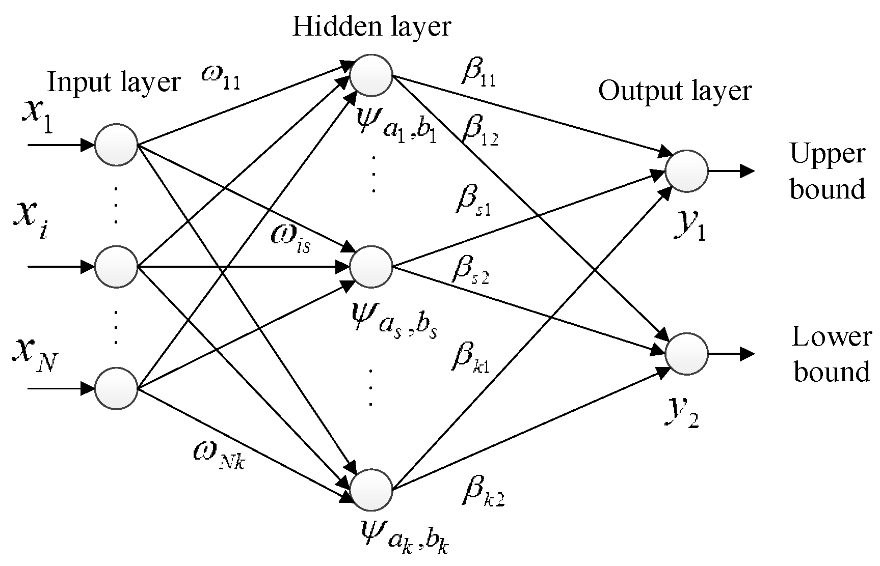
3.2. WNN-Based PI Construction

WNN is a neural network based on the wavelet transform (WT). It is powerful for frequency component analysis and suitable for signals which are composed of high-frequency components with short duration and low-frequency components with long duration [20,21]. A brief review of WT is described as follows:
Assuming that f ( t ) is a square integral function, it can be expressed as:
f ( t ) = W ( a , b ) ψ ( t b a ) d b d a
where W ( a , b ) is the continuous wavelet transformation of f ( t ) and defined as:
W ( a , b ) = f ( t ) ψ a , b * ( t ) d t
with:
ψ a , b * ( t ) = 1 a ψ ( t b a )
where a and b are the scaling parameter and shifting parameter, respectively.
X i = { x 1 , , x i , , x N } is the N input sample of WNN, ω i s is the input parameter between the input layer node and the hidden layer node, and β s j is the output parameter that connects the hidden layer and the output layer. The calculation equation of the output of the hidden layer is as follows:
g ( s ) = ψ ( ( i = 1 N ω i s x i b s ) / a s ) , s = 1 , 2 , k
where g ( s ) is the output of the s node of the hidden layer, ψ is the small wave basis function, and k is the number of hidden layer nodes of the WNN. The calculation equation of the output layer is as follows:
Y j = s = 1 k β s j g ( s ) , s = 1 , 2 , k
Then, the M output Y j = { y 1 , , y j , , y M } of the WNN is designed as:
y j = s = 1 k β s j ψ ( ( i = 1 N ω i s x i b s ) / a s )
The upper and lower bounds of the prediction interval of wind power are directly given by the dual-output WNN, which effectively avoids the complex process of the traditional interval prediction method for the probability error analysis. Thus, a symbolic WNN-based on PIs’ construction model is shown in Figure 1.
In order to avoid the irrational effect of the number of input and hidden layer nodes on the prediction results, the C-C phase space reconstruction method is used to determine the number of input layer nodes N. According to the Kolmogorov theorem, the number of hidden layer nodes K is determined, and the structure of the PI model for the WNN is N–K–2. The Morlet wavelet with strong adaptive ability is selected as the wavelet basis function, and the equation is as follows:
ψ ( t ) = cos ( 1.75 t ) e t 2 / 2
By choosing suitable input parameters, output parameters, scaling parameters, and shifting parameters of the WNN, effective and reliable PIs of wind power will be constructed.

4. Evolution Knowledge MOABC Algorithm (EKMOABC) for WNN-Optimized Construction of PIs

To choose the parameters of WNN reasonably and solve the multi-objective optimization problem for PI construction, an improved MOABC algorithm, called Evolution Knowledge MOABC (EKMOABC), is proposed. The main steps of EKMOABC are summarized as follows:

4.1. Initialization

The input parameters, the output parameters, the scaling parameters and shifting parameters of WNN are initialized at this step. The wind power data are divided into a training set, a validation set, and a test set, and then they are normalized to [ 0 , 1 ] . The parameters of EKMOABC, including the number of food sources N , the maximum iterations T m , the maximum number of solutions in archive I m , the maximum obsolete number of scout bees D m , the probability parameters η 1 and η 2 , are also initialized.

4.2. Preliminary Iteration

Preliminary iteration is crucial for the repeatability of the model. Firstly, each food source is initialized as:
x i j = L + r a n d ( 0 , 1 ) × ( U L )
where x i j is one of the food sources. i 1 , 2 , , N / 2 , j 1 , 2 , , D and D is the number of parameters to be optimized. L and U are the minimum lower bound and maximum upper bound of the solutions, respectively. Then the assessment criteria PICP and PICAW are calculated.

4.3. Pareto Dominance

Compared with single-objective optimization, the solution of the multi-objective optimization problem is a trade-off of the performance, which is called the Pareto optimal set based on Pareto dominance.
For the decision vector x a , x b Ω , x a dominates x b (denoted as x a x b ) if f i ( x a ) f i ( x b ) and f i ( x a ) < f i ( x b ) . Therefore, a set of decision vectors ν Ω is called a non-dominate solution when ¬ x Ω : x v . Furthermore, a Pareto optimal front set is defined as a group of non-dominate solutions.
In this paper, α and PICAW are the optimization objectives. Thus, when the objectives satisfy the equation below:
α i α j , PICAW i PICAW j
where α and PICAW cannot be met simultaneously, it is said that the solution i dominates solution j , which can be denoted as i j . When the dominant relationship of different food sources is achieved, the non-dominate solution is chosen into the archive.

4.4. Employed Bees Evolution Based on Guidance of Elite Population Knowledge

Elite population represents the optimal information of population and it is beneficial for the population to converge rapidly [20]. Thus, a more effective strategy is adopted to choose an elite population and guide the employed bees’ evolution. In the first iteration, the crowding distance of solutions in the archive is calculated and the maximum crowding distance is chosen as the elite solution. Additionally, objective functions should be ordered first according to Equation (16) when the crowding distance is calculated. The crowding distance is defined as:
d i = { 1 2 k = 1 m ( ( f i k f i k 1 ) 2 + ( f i k f i k + 1 ) 2 ) , 1 < i < s inf , e l s e
where f i k is the target value (the assessment criteria of PIs). m is the number of the target value. s is the number of solutions in the archive. At the next iteration, an elite solution will be chosen and compared with the former one. When the new elite solution dominates the old one, it will be saved and guide the employed bees’ evolution instead. Otherwise, the old one will be saved. However, when neither elite solution dominates the other one, the roulette method will be adopted for making the decision.
In this paper, both dominant and non-dominant solutions of employed bees evolve in different ways. The evolution method is as follows:
{ ν t j = x t j + r 1 ( x t j x k j ) + r 2 ( x t j x b j ) , s i = 0 v f = x f + r 3 ( x f x b ) , s j = 1
where s i is a flag. s i = 0 represents the dominant solution, while s j = 1 represents the non-dominant solution. x b is the elite solution. x t and x f are the non-dominant solution, and t f . r 1 , r 2 , r 3 [ 1 , 1 ] . This measure is applied in both the dominated front and non-dominated front. When the non-dominant solutions crossover with the elite solution, it is easier to produce excellent solutions and keep the elite population alive. On the other hand, when dominant solutions crossover with both the elite solution and the non-dominant solution, it is beneficial to maintain the diversity of the population.

4.5. Probability Choice Equation Combining the Dominance and Distribution Relationships

Probability choice equation is used to choose the solutions to evolve deeply and balance the capacity between exploit and explore. Different from the single-objective optimization, there may be a large number of solutions for multi-objective optimization which cannot dominate other solutions at the same time. The quality of the Pareto optimal set is related to both the dominance relationship and distribution relationship. If only one of them is considered in the probability choice equation, it will hardly obtain the high-quality of PIs. Therefore, a typical probability choice equation combining the dominance and distribution relationships is proposed as follows:
P i = { 1 1 + ( 1 s i ) e η 1 l i , s i = 0 1 1 + s i e η 2 d i , s i = 1
where P i is the probability, d i is the crowding distance. η 1 and η 2 are the probability choice parameters and l i is defined as:
l i = min j = 1 s k = 1 m ( f i k f j k ) 2
where f i is the dominant solution and f j is the non-dominant solution. s is the number of solutions in the archive.
From Equations (18) and (19), we can see that the proposed equation of probability choice combines the dominance relationship and the distribution relationship. When the solution is dominated by other solutions, it will be punished by the distance from the Pareto optimal set. From Equation (18), when the solution is dominated, the probability will be limited to [ 0 , 0.5 ] by the parameter η 1 . However, when the solution is non-dominated, the probability will be chosen in the range of [ 0.5 , 1 ] due to the superiority of non-dominant solutions. Thus, even though the dominant solution is closer to the Pareto optimal set, its probability will be never be greater than that of the non-dominant solution, which will be of great benefit for population evolution both in convergence and distribution.

4.6. Onlooker Bees Evolution

Onlooker bees evolve through the roulette method according to the probability calculated above. The evolution method of onlooker bees is the same as the employed bees.

4.7. Strategy to Update the Archive

The archive is used to save the best solutions ever found and the final solutions in the archive are called the Pareto optimal set. Thus, the strategy for updating the archive is crucial for the quality of the results. Traditionally, the non-dominant solutions are chosen for the archive and weeded out when it is dominated or the crowding distance is too small. In the preliminary iteration, there are few non-dominant solutions and it is reasonable to update the archive. However, in the later iterations, the amount of non-dominant solutions increases quickly, which means some better solutions should be chosen for the archive and some would be deleted. Then the cost of using the traditional strategy will increase. Thus, a stricter strategy is chosen to update the archive. When the number of solutions in the archive reaches the maximum value I m , the solutions with the smallest crowding distance will be deleted, and the maximum crowding distance of these deleted solutions are calculated and recorded as d t max . When a solution satisfies the condition for being saved into the archive, one stricter step will be checked. Firstly, the distance between this solution and the other solutions in the archive is calculated. Then the minimum distance will be recorded as d t min and only when d t min > d t max , the solution can be chosen to be saved into the archive. The new strategy for archive updating reduces the cost of the algorithm and improves the distribution performance of the Pareto optimal set.

4.8. Scout Bees Evolution

When the evolution of the employed bees and onlooker bees are completed and the solution is not improved, the number of obsolete scout bees will be added by 1. Once it reaches its maximum value D m , the employed bees will be transformed into scout bees to produce a new solution randomly.

4.9. Termination

The condition for finishing the algorithm is that the iterations reach its maximum value T m .

5. Experiments and Results

To validate the multi-objective optimization model for PI construction, the wind power data sampled every 10 min from the Alberta interconnected electric system in 2015 are applied. A total of 6000 datasets from 1 January are chosen as the research data with 80% for training and the other 20% for validating and testing, respectively. Firstly, the datasets are normalized in [ 0 , 1 ] to adjust the parameters of WNN and avoid the influence from different magnitudes of the datasets. Then the structure of WNN using the Morlet wavelet as the basic wavelet is determined. It is necessary to balance the complexity and the learning capacity of WNN. The C-C phase space reconstruction and Kolmogorov theorem are adopted to choose the optimal WNN structure as 4-8-2. Finally, the parameters of WNN and EKMOABC will be set as mentioned in Section 4.
The CWC for PI construction is a single-objective optimization problem, while PIMOC is a multi-objective optimization problem. To valid the experiment results, the basic ABC algorithm in [21] is used to optimize the CWC, and the MOABC algorithm in [22] to optimize the WNN for PIMOC. The food source number of ABC and MOABC are both set to 40, the maximum iteration time is set to 200, the maximum number of solutions in the archive is 20, and the maximum number of obsolete scout bees is 50.

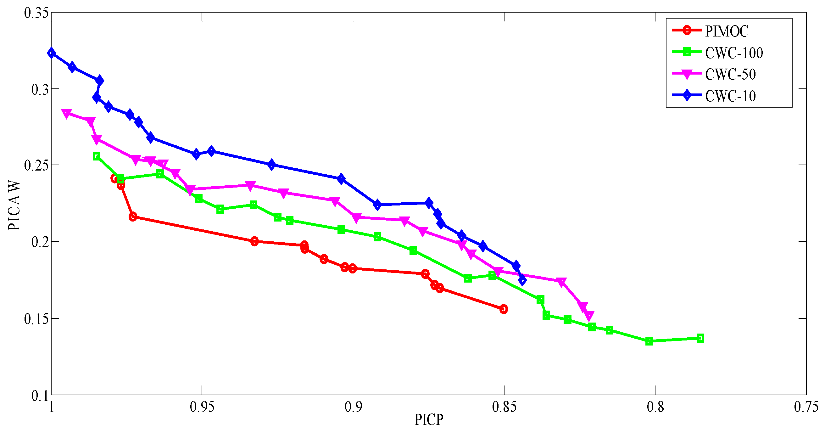
5.1. Performance Comparisons between CWC with Different Parameters and PIMOC

To validate the influences of parameters on CWC, the control parameter η in Equation (5) is chosen as η = 10 ,   50 ,   100 and μ is set as 80%, 85%, 90%, 95%, and 99%. Each experiment is repeated 10 times with different η and μ . The average results are shown in Table 1.
From Table 1, it is obvious that PICP increases with the increase of μ when η is fixed, and PICAW also becomes larger, which makes the accuracy of the PIs worse. On the other hand, η has a great effect on the quality of PIs with the fixed μ . A small η is helpful to improve the accuracy of PIs with a small width of PIs, but it is difficult to ensure that PICP reaches its expected μ and meets the reliability requirements of the PIs. A large η can enhance the reliability of the PIs, and the PICP is always higher than its expected value. However, this will lead to a large width of the PIs, which then makes the solving process into a local optimum. Thus, the controlling parameter η is an uncertain factor in PI construction with CWC, which is unfavorable for solving this optimization problem in high quality.
In order to compare the prediction results between CWC (with the ABC-WNN as the prediction model) and PIMOC (with the MOABC-WNN as the model), the experiments with a group of μ (from 80–99%) in different η are performed and the results are shown in Figure 2.
As is shown in Figure 2, the prediction results of PIMOC are better than CWC both in the criteria of PICP and PINAW. With different η , the PICP and PICAW of CWC change greatly. During the optimization of CWC, the solutions that cannot satisfy the given confidence level μ will be penalized by η and determined whether to be saved or not according to η . Perhaps a large η can ensure that the requirement of the confidence level μ should be met, but some good solutions which have a PICP slightly less than its expected value, but a good PI width, will be weeded out. However, if a small η is chosen and then the solutions with a slightly worse confidence level, but a small width of the PIs is saved, those solutions dissatisfy the requirement of the confidence level and will not be penalized sufficiently. As a result, the confidence level of all the solutions will be lowered. Thus, a suitable η is of great significance to CWC, but it is always chosen empirically. In PIMOC, this multi-objective optimization problem is solved by adopting a multi-objective evolution algorithm directly instead of transforming it into a single-objective optimization problem, which avoids the choosing of η and it is a benefit for improving the quality of PIs both in accuracy and reliability.
For a better explanation, the PIs of CWC are shown in Figure 3, Figure 4 and Figure 5 with three different η (the value of η is same as it in Table 1) and the PIs of PIMOC are shown in Figure 6, where Pareto optimal sets are sorted in ascending order according to PICP and the first, fifth, tenth, fifteenth, and twentieth PIs are plotted to make a comparison with the PIs of CWC.
As is shown in Figure 3, Figure 4 and Figure 5, with the control parameter η increasing, the prediction accuracy of the PIs is improved, while the width is larger and the reliability becomes worse, which is just the same as in Table 1. An unreasonable choice of η may easily cause some excellent solutions unreserved in the next iteration. From Equation (5), it can be seen that, in CWC, the quality of the PIs is assessed impartially only based on a single synthetical criterion. While in PIMOC, some excellent solutions are reserved by the Pareto dominance strategy avoiding the choice of η , and the assessment is carried out according to both PIMOC, both in accuracy and reliability. Then we can see that the performances of PIMOC in Figure 6 are better than all those of CWC in Figure 3, Figure 4 and Figure 5.

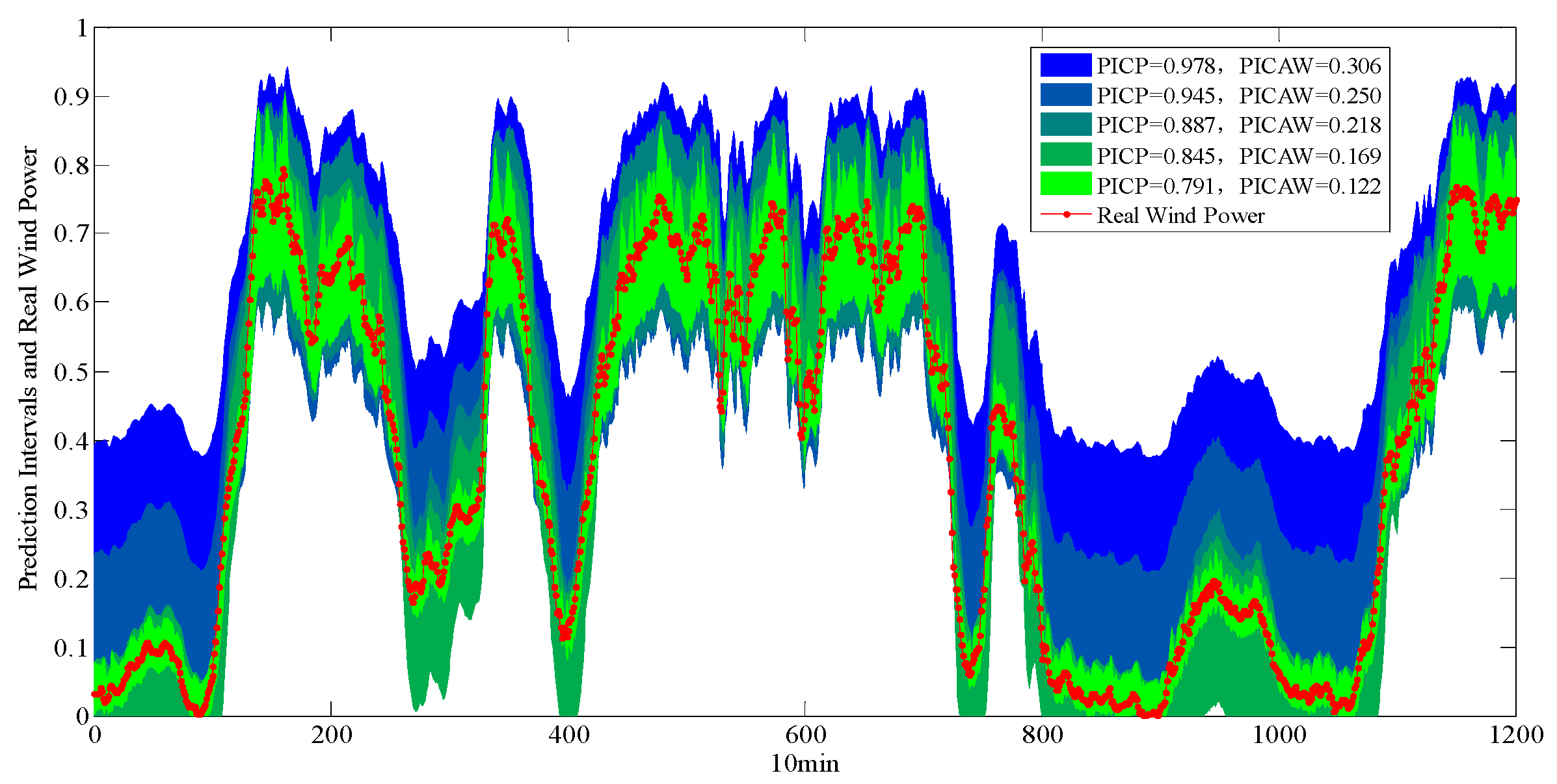
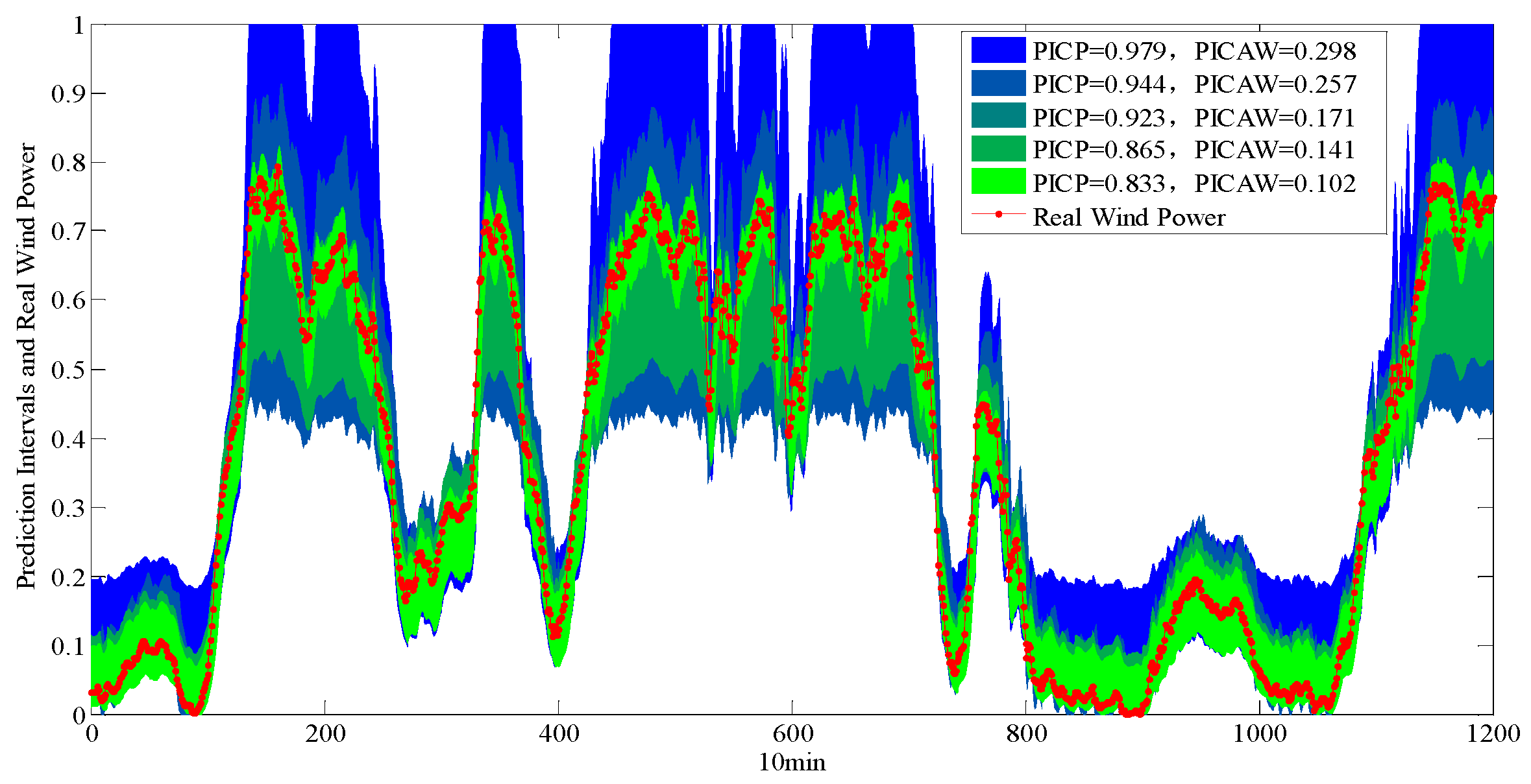
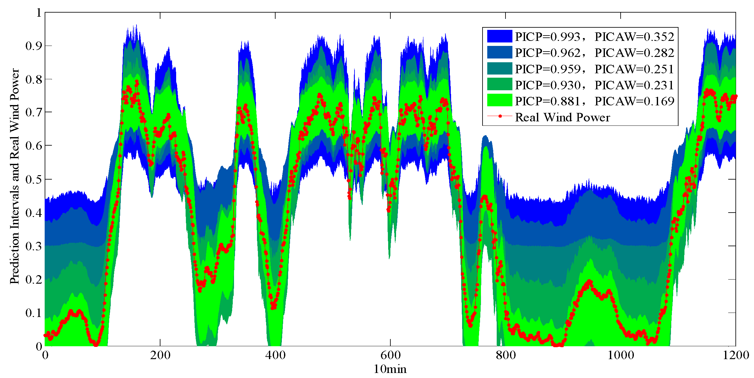
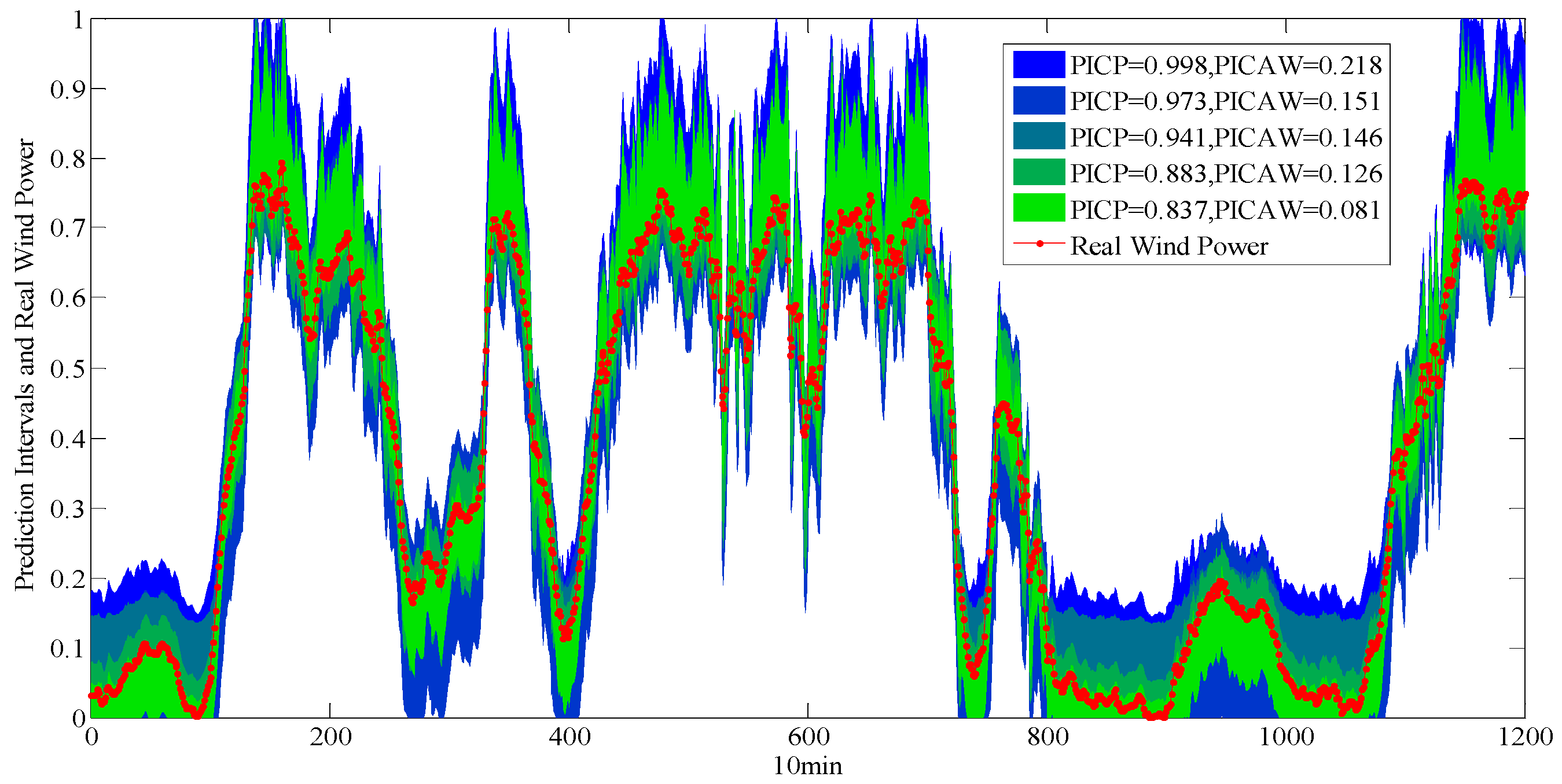
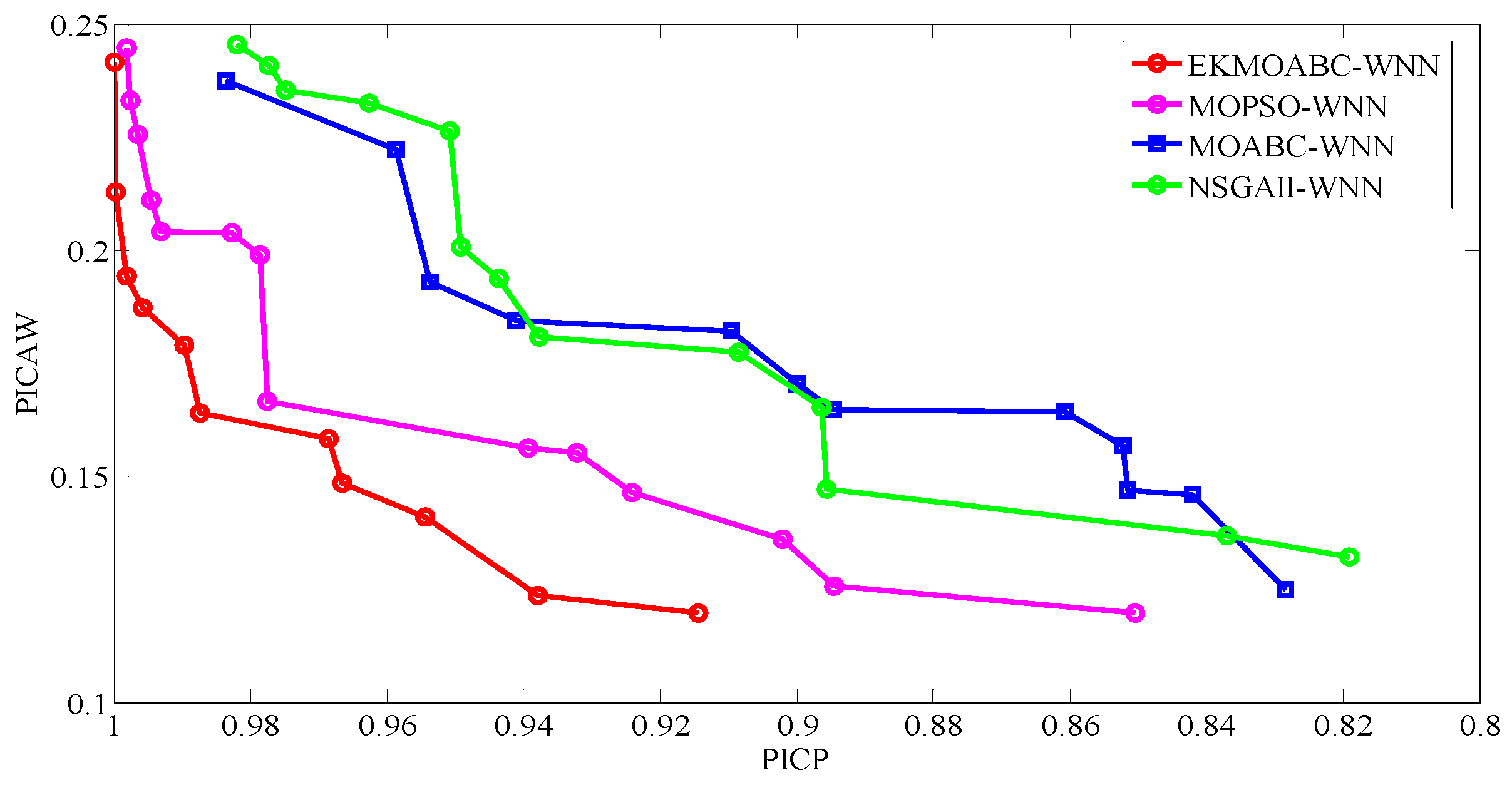
5.2. Performances of the Multi-Objective Evolution Algorithm in PI Construction

To evaluate the proposed EKMOABC for solving the multi-objective optimization problem with PIMOC, three classic multi-objective optimization algorithms, including the basic MOABC, NSGAII (non-dominated sorting genetic algorithm II) [23], and MOPSO (multi-objective particle swarm optimization) [24], are used to optimize the parameters of WNN for contrast experiments. The population size, the maximum number of iterations, and the maximum number of solutions in the archive are set to 40, 200, 20, respectively, for all algorithms. The crossover probability and the mutation probability of NSGAII are set to 0.8 and 0.2, respectively. The inertia weight and the learning factor of MOPSO are set to 0.8 and 2, respectively. The probability choices parameter η 1 and η 2 of EKMOABC are set to 50 and 10. The maximum obsolete number of scout bees in MOABC and EKMOABC are all set to 50. The comparative results for PI construction with four different multi-objective evolutionary optimization algorithms are shown in Figure 7.
As shown in Figure 7, Compared with the other three evolutionary optimization algorithms (NSGAII, MOPSO, and MOABC) in WNN optimization, the proposed EKMOABC-WNN can ensure a higher confidence level and narrower width of PIs, especially when the PICP is above 97%, where there is no suitable width of PIs that can be chosen by the other three algorithms. The Pareto optimal set with EKMOABC-WNN has not only better convergent performance, but also distributing performance. One of the reasons is that NSGAII, MOPSO, and MOABC may be easily trapped into a local optimum and their searching capacities will become so weak that the better solutions cannot be searched in the constraint range. Another reason is that the distribution of the Pareto set is not considered sufficiently in the process of iteration in NSGAII, MOPSO, and MOABC, which results in the Pareto set non-uniform distribution. In addition, the EKMOABC is based on the relationship between Pareto domination and distribution. The advanced probability choice equation of EKMOABC can avoid the solutions being trapped into local optimum effectively and it is a benefit for the distribution of the Pareto optimal set. The strategy of the guidance with elite population knowledge plays an important role in searching for better solutions and improving the convergent performance of the Pareto optimal set.

6. Conclusions

Wind power forecasting is of great importance for electrical power systems because of the uncertainties of climate, especially when the renewable energies are merged into the grid. Compared with point forecasting, PI forecasting is an effective way for assessing the uncertainty of wind power. However, the traditional method for prediction interval construction is carried out under some special assumptions and suffers from computational complexity. In this paper, an improved MOABC method was proposed to optimize the parameters of WNN for PI construction in wind power. Instead of transforming into a single-objective optimization problem, the primary multi-objective optimization problem is solved directly by the improved MOABC, called EKMOABC. In addition, a new multi-objective criterion, called PIMOC, was proposed, with which the effect of the prediction value of the PIs is considered. Comparative results between CWC and PIMOC in PI construction demonstrate that the CWC is affected by the controlling parameter η greatly while the PIMOC can avoid the choice of this parameter, so the quality of the PIs based on PIMOC is more accurate and reliable. On the other hand, a multi-objective algorithm, called EKMOABC, was also proposed for the solutions of PIMOC. Some simulation experiments comparing with NSGAII, MOPSO, and MOABC showed that the EKMOABC-based WNN for wind power PI forecasting has a narrower width and higher confidence, which means higher accuracy and reliability.

Acknowledgments

This work was supported in part by the National Nature Science Foundation under grant 61573167 and grant 61572237, in part by the Fundamental Research Funds for the Central Universities under grant JUSRP31106 and grant JUSRP51510, and in part by the Postgraduate Research and Practice Innovation Program of Jiangsu Province under grant KYCX17_1488.

Author Contributions

Yanxia Shen conceived the experiment and wrote the paper; Xu Wang helped in the experiment and writing; and Jie Chen performed the experiments.

Conflicts of Interest

The authors declare no conflict of interest.

References

  1. Wang, Q.; Martinez-Anido, C.B.; Wu, H.; Florita, A.R.; Hodge, B.M. Quantifying the economic and grid reliability impacts of improved wind power forecasting. IEEE Trans. Sustain. Energy 2016, 7, 1525–1537. [Google Scholar] [CrossRef]
  2. Tascikaraoglu, A.; Uzunoglu, M. A review of combined approaches for prediction of short-term wind speed and power. Renew. Sustain. Energy Rev. 2014, 34, 243–254. [Google Scholar] [CrossRef]
  3. Haque, A.U.; Nehrir, M.H.; Mandal, P. A hybrid intelligent model for deterministic and quantile regression approach for probabilistic wind power forecasting. IEEE Trans. Power Syst. 2014, 29, 1663–1672. [Google Scholar] [CrossRef]
  4. Hu, J.; Wang, J. Short-term wind speed prediction using empirical wavelet transform and Gaussian process regression. Energy 2015, 93, 1456–1466. [Google Scholar] [CrossRef]
  5. Che, Y.; Peng, X.; Monache, L.D.; Kawaguchi, T.; Xiao, F. A wind power forecasting system based on the weather research and forecasting model and Kalman filtering over a wind-farm in Japan. J. Renew. Sustain. Energy 2016, 8, 319–329. [Google Scholar] [CrossRef]
  6. Zuluaga, C.D.; Álvarez, M.A.; Giraldo, E. Short-term wind speed prediction based on robust Kalman filtering: An experimental comparison. Appl. Energy 2015, 156, 321–330. [Google Scholar] [CrossRef]
  7. Yan, J.; Li, K.; Bai, E.; Yang, Z.; Foley, A. Time series wind power forecasting based on variant Gaussian Process and TLBO. Neurocomputing 2016, 189, 135–144. [Google Scholar] [CrossRef]
  8. Zhao, Y.; Ye, L.; Li, Z.; Song, X.; Lang, Y.; Su, J. A novel bidirectional mechanism based on time series model for wind power forecasting. Appl. Energy 2016, 177, 793–803. [Google Scholar] [CrossRef]
  9. Osório, G.J.; Matias, J.C.O.; Catalão, J.P.S. Short-term wind power forecasting using adaptive neuro-fuzzy inference system combined with evolutionary particle swarm optimization, wavelet transform and mutual information. Renew. Energy 2015, 75, 301–307. [Google Scholar] [CrossRef]
  10. Ata, R. Artificial neural networks applications in wind energy systems: A review. Renew. Sustain. Energy Rev. 2015, 49, 534–562. [Google Scholar] [CrossRef]
  11. Li, S.; Wang, P.; Goel, L. Wind power forecasting using neural network ensembles with feature selection. IEEE Trans. Sustain. Energy 2017, 6, 1447–1456. [Google Scholar] [CrossRef]
  12. Tewari, S.; Geyer, C.J.; Mohan, N. A statistical model for wind power forecast error and its application to the estimation of penalties in liberalized markets. IEEE Trans. Power Syst. 2011, 26, 2031–2039. [Google Scholar] [CrossRef]
  13. Quan, H.; Srinivasan, D.; Khosravi, A. Short-term load and wind power forecasting using neural network-based prediction intervals. IEEE Trans. Neural Netw. Learn. Syst. 2014, 25, 303. [Google Scholar] [CrossRef] [PubMed]
  14. Quan, H.; Srinivasan, D.; Khosravi, A. Incorporating wind power forecast uncertainties into stochastic unit commitment using neural network-based prediction intervals. IEEE Trans. Neural Netw. Learn. Syst. 2015, 26, 2123–2135. [Google Scholar] [CrossRef] [PubMed]
  15. Quan, H.; Srinivasan, D.; Khosravi, A. Particle swarm optimization for construction of neural network-based prediction intervals. Neurocomputing 2014, 127, 172–180. [Google Scholar] [CrossRef]
  16. Khosravi, A.; Nahavandi, S.; Creighton, D.; Atiya, A.F. Lower upper bound estimation method for construction of neural network-based prediction intervals. IEEE Trans. Neural Netw. 2011, 22, 337–346. [Google Scholar] [CrossRef] [PubMed]
  17. Khosravi, A.; Nahavandi, S.; Creighton, D. Construction of optimal prediction intervals for load forecasting problems. IEEE Trans. Power Syst. 2010, 25, 1496–1503. [Google Scholar] [CrossRef]
  18. Catalão, J.P.S.; Pousinho, H.M.I.; Mendes, V.M.F. Short-term wind power forecasting in Portugal by neural networks and wavelet transform. Renew. Energy 2011, 36, 1245–1251. [Google Scholar] [CrossRef]
  19. Rafiei, M.; Niknam, T.; Khooban, M.H. Probabilistic forecasting of hourly electricity price by generalization of elm for usage in improved wavelet neural network. IEEE Trans. Ind. Inform. 2016, 13, 71–79. [Google Scholar] [CrossRef]
  20. Ibrahim, A.; Rahnamayan, S.; Martin, M.V.; Deb, K. Elite NSGA-III: An improved evolutionary many-objective optimization algorithm. In Proceedings of the 2016 IEEE Congress on Evolutionary Computation (CEC), Vancouver, BC, Canada, 24–29 July 2016; pp. 973–982. [Google Scholar] [CrossRef]
  21. Karaboga, D.; Gorkemli, B. A quick artificial bee colony (qABC) algorithm and its performance on optimization problems. Appl. Soft Comput. J. 2014, 23, 227–238. [Google Scholar] [CrossRef]
  22. Akbari, R.; Hedayatzadeh, R.; Ziarati, K.; Hassanizadeh, B. A multi-objective artificial bee colony algorithm. Swarm Evol. Comput. 2012, 2, 39–52. [Google Scholar] [CrossRef]
  23. Deb, K.; Pratap, A.; Agarwal, S.; Meyarivan, T. A fast and elitist multi-objective genetic algorithm: NSGA-II. IEEE Trans. Evol. Comput. 2002, 6, 182–197. [Google Scholar] [CrossRef]
  24. Coello, C.A.C.; Pulido, G.T.; Lechuga, M.S. Handling multiple objectives with particle swarm optimization. IEEE Trans. Evol. Comput. 2004, 8, 256–279. [Google Scholar] [CrossRef]
Figure 1. WNN-based on the PI construction model. WNN: wavelet neural network; PI: prediction interval.
Applsci 08 00185 g001
Figure 2. Comparative results between CWC and PIMOC. CWC: coverage width-based criterion; PIMOC: PIs’ multi-objective optimization criteria; PICP: PI coverage probability.
Applsci 08 00185 g002
Figure 3. Prediction intervals with CWC ABC-based when η = 10 . CWC: coverage width-based criterion; ABC: artificial bee colony; PICAW: PIs covered-normalized average width; PICP: PI coverage probability.
Applsci 08 00185 g003
Figure 4. Prediction intervals with CWC ABC-based when η = 50 . CWC: coverage width-based criterion; ABC: artificial bee colony; PICAW: PIs covered-normalized average width; PICP: PI coverage probability.
Applsci 08 00185 g004
Figure 5. Prediction intervals with ABC-based CWC when η = 100 . CWC: coverage width-based criterion; ABC: artificial bee colony; PICAW: PIs covered-normalized average width; PICP: PI coverage probability.
Applsci 08 00185 g005
Figure 6. Prediction intervals with PIMOC based on MOABC. PIMOC: PIs’ multi-objective optimization criteria; MOABC: multi-objective artificial bee colony; PICAW: PIs covered-normalized average width; PICP: PI coverage probability.
Applsci 08 00185 g006
Figure 7. Comparative results with different multi-objective evolutionary algorithms. EKMOABC: evolutionary knowledge multi-objective artificial bee colony; MOPSO: multi-objective particle swarm optimization; MOABC: multi-objective artificial bee colony; NSGAII: non-dominated sorting genetic algorithm II; PICAW: PIs covered-normalized average width; PICP: PI coverage probability.
Applsci 08 00185 g007
Table 1. Comparative results with different η and μ of CWC. CWC: coverage width-based criterion; PICP: prediction interval coverage probability; PICAW: prediction intervals covered-normalized average width.
μ Name μ = 0.80 μ = 0.85 μ = 0.90 μ = 0.95 μ = 0.99
η
η = 10 PICP0.7850.8360.8920.9440.985
PICAW0.1370.1520.2030.2350.256
η = 50 PICP0.8220.8640.9230.9630.995
PICAW0.1520.1980.2320.2510.284
η = 100 PICP0.8440.8720.9470.9811.000
PICAW0.1750.2180.2590.2880.323

