Statistical, Spatial and Temporal Mapping of 911 Emergencies in Ecuador
by
 , ,
, ,
Danilo Corral-De-Witt
1,2,* ,
,
Enrique V. Carrera
1 ,
,
Sergio Muñoz-Romero
2,3 and
José Luis Rojo-Álvarez
2,3 1
Departamento de Eléctrica y Electrónica, Universidad de las Fuerzas Armadas ESPE, 171103 Sangolqui, Ecuador
2
Departamento de Teoría de la Señal y Comunicaciones, Sistemas Telemáticos y Computación, Universidad Rey Juan Carlos, 28943 Fuenlabrada, Spain
3
Center for Computational Simulation, Universidad Politécnica de Madrid, Boadilla del Monte, 28660 Madrid, Spain
*
Author to whom correspondence should be addressed.
Appl. Sci. 2018, 8(2), 199; https://doi.org/10.3390/app8020199
Submission received: 9 January 2018
/
Revised: 25 January 2018
/
Accepted: 26 January 2018
/
Published: 29 January 2018
Abstract
:A public safety answering point (PSAP) receives alerts and attends to emergencies that occur in its responsibility area. The analysis of the events related to a PSAP can give us relevant information in order to manage them and to improve the performance of the first response institutions (FRIs) associated to every PSAP. However, current emergency systems are growing dramatically in terms of information heterogeneity and the volume of attended requests. In this work, we propose a system for statistical, spatial, and temporal analysis of incidences registered in a PSAP by using simple, yet robust and compact, event representations. The selected and designed temporal analysis tools include seasonal representations and nonparametric confidence intervals (CIs), which dissociate the main seasonal components and the transients. The spatial analysis tools include a straightforward event location over Google Maps and the detection of heat zones by means of bidimensional geographic Parzen windows with automatic width control in terms of the scales and the number of events in the region of interest. Finally, statistical representations are used for jointly analyzing temporal and spatial data in terms of the “time–space slices”. We analyzed the total number of emergencies that were attended during 2014 by seven FRIs articulated in a PSAP at the Ecuadorian 911 Integrated Security Service. Characteristic weekly patterns were observed in institutions such as the police, health, and transit services, whereas annual patterns were observed in firefighter events. Spatial and spatiotemporal analysis showed some expected patterns together with nontrivial differences among different services, to be taken into account for resource management. The proposed analysis allows for a flexible analysis by combining statistical, spatial and temporal information, and it provides 911 service managers with useful and operative information.
1. Introduction
Since the 1950s, emergency services have been operating in North America mostly through a unique three-digit number (e.g., 911) for easy memorization, allowing anyone at anytime to contact a call-taker located in a public safety answering point (PSAP). A PSAP is a facility at which emergency calls are received under the responsibility of a public authority [1]. From this facility, a diversity of first response institutions (FRIs) can be coordinated and dispatched, according to the type of reported emergency. Among the main FRIs, we can find police, medical services, or fire brigades. The first generation of 911 services used the public switched telephone network (PSTN) to receive alert calls in the PSAPs [2]. When cellular communications arrived, these services evolved to enhanced 911 (E-911), with the aim of incorporating and supporting calls made from mobile devices, which have different operation schemes and protocols relative to landlines [3]. The latest technological advances in communications have generated next-generation 911 (NG-911) services, which have enabled the use of Internet protocols for transmitting voice, video, and text messages for emergency communications [4]. These new emergency response services are operating in many countries around the world, including the Integrated Security Service ECU 911 (where ECU is an abbreviation for Ecuador), which began its operations in this country in 2012.
All of these emergency services handle a large amount of information with complex geographical and temporal heterogeneities. The information stored in event databases (DBs) at each PSAP has mostly been used for generating numerical reports of events attended by each FRI in a descriptive form. However, it becomes clearer every day that many more benefits can be obtained by exploiting the dynamically stored data in order to provide service managers with efficient tools for analyzing the complex event dynamics and their interactions, rather than limiting ourselves to summary reports [5]. Thus, it seems possible to increase the quality and efficiency of the stored-data analysis by combining statistical, spatial, and temporal information for a better understanding of the attended emergencies, for generating useful reports, and for improving resource management [6,7,8]. This analysis will increase the response capacity of the FRIs, optimizing available resources, shortening response times, and helping to plan the response to similar events in the future on the basis of the analysis of historical data [9].
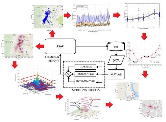
Therefore, this work proposes an analysis system to scrutinize the available information regarding emergencies attended by a PSAP. We used a set of techniques for the simple and effective representation of emergency events using statistical, temporal, and geographical analysis. The implemented model was oriented to obtain a statistical and spatial–temporal characterization of the continuous operation of FRIs. We designed the system and developed a case study by using the information of more than 1 million emergencies attended during 2014 by the E-911 PSAP of Quito, Ecuador. The selected and designed temporal analysis tools included seasonal representations and nonparametric confidence intervals (CIs), which allowed us to dissociate the main temporal components from transients. The spatial analysis tools included a straightforward event location over Google Maps and the detection of heat zones by means of bidimensional geographic Parzen windows with automatic width control in terms of scales and the number of events in a region of interest. Finally, statistical representations are used for jointly analyzing time and space in terms of the “time–space slices”.
This paper is organized as follows. Section 2 describes the emergency representation model and the operation of a PSAP. In Section 3, the behaviors of different FRIs are described, several examples of the emergencies attended during 2014 are analyzed, and the main results are explained and discussed. Finally, conclusions and future work are presented in Section 4.
2. Emergency Representation Model
This section starts by describing the operation of the Ecuadorian 911 service in order to give a better understanding of the requirements and needs of this type of system. After this system description, we present an equation notation for event sets, and we use it to represent the seasonal evolution and the nonparametric CIs on the temporal representation. Then, the well-known Parzen window model is used to support the geographical representation of each event set. Finally, a representation is provided for the straightforward statistical visualization of joint temporal and spatial event density, given by spatial–temporal slices of the Parzen windows.
2.1. Operation of a PSAP at ECU 911
According to the management model developed for the ECU 911, each PSAP has a specific coverage area. During normal operation, all the alert calls are routed by the PSTN or cellular network to the nearest PSAP, at which evaluation groups receive and analyze the content of every alert; when it does not proceed, the call is saved for its posterior classification and processing. If the alert proceeds, it is automatically turned into an emergency and is transferred to the corresponding FRI. Then, the dispatching evaluator of the particular institution decides which resources will be moved to attend the emergency and whether it is necessary to coordinate with other FIRs, according to the emergency’s relevance and affectation. This operation process is summarized in Figure 1a. The received alerts can originate from landline calls, cellphone calls, emergency buttons, reports from a member of a FRI, or detection by a surveillance camera evaluator.
A relevant point in an emergency system description is the percentage of the participation of each FRI in the total number of emergencies attended in a PSAP. For the case of Quito, Ecuador, this information can be readily obtained from the statistics section of the ECU 911 Website [10]. As we can see in Table 1, from more than 1 million emergencies registered during 2014, the group including police, health, and transit services represented 92% of the emergencies. On the other hand, fire brigades, municipal services, risk management secretaries (RMSs), and military forces only represented the remaining 8%. The Integrated Security Service has created a dictionary that defines 121 variables used to characterize the attended emergencies. Filtering the information contained in these variables, it is possible to identify very specific events, details, and any other important information regarding with the emergency.
Thus, the proposed event analysis system is illustrated in Figure 1b. The information of all the attended emergencies is saved in an SQL DB at each PSAP. For this work, a report of the emergencies attended by the PSAP in Quito was downloaded in a CSV file. Using Matlab® software (version 2017b, The Mathworks, Nattic, MA, USA, 2017), we organized the emergencies according to the parameters that we wanted to analyze in a .mat file. Temporal, geographical, and statistical analyses were developed and combined in order to model the behavior of each FRI. The results of this analysis could be subsequently used to send feedback to the PSAP managers, aiming to improve the response of the FRIs.
The information regarding any emergency contains a register with times associated to all the instances produced in the PSAP (i.e., the time when the alert arrives, when it is transferred to the FRI, when the resource is dispatched, when the resource arrives at the event site, and when the emergency is closed with a report of results). With this information, it is possible to map the events within a given geographical region by chronological order and filter the emergencies by the year, month, day, or even hour. This analysis allows managers to understand the temporal behavior of the emergencies attended by each FRI. Examples of this kind of representation are illustrated in Figure 2, where it is possible to identify the emergencies that occurred during the third week of January, and they are represented by days and hours next to their map localizations.
2.2. Temporal Event Analysis
From a mathematical point of view, we have a set of N observed events for all the institutions, and each event has been registered at time , . We denote by the subset of events corresponding to the ith institution, where , and L is the total number of institutions. According to this, and considering that each event occurs at a specific time and in a specific geographical location, we denote an event as , where denotes the bivariate Dirac delta function [11]. Its first argument accounts for the time evolution, while the second accounts for the geographical location of each event. We note that denotes the coordinate vector of an event in general terms, which will be on the earth’s surface, specifying the place of the event’s occurrence and expressed in some adequate coordinate system. Thus, the original event series is given by the accumulation of shifted bivariate deltas:
whereas the set of events for the ith institution can be expressed as
where denotes the set of indices belonging to the ith institution in the system. We can obtain an expression for the time evolution of the event series in M intervals, for the ith institution, by establishing a time interval width T and a spatial integration domain . This is
where
and is thus obtained as the number of events available in the dataset in the time period m () and in the spatial domain when an observation time width T is used.
With this simple event description in the temporal domain, time averages can be obtained and estimated from the available set of observations through
We note that E denotes here the theoretical statistical expectation; however, it is not available in our problem. Instead, we constrain ourselves to working with the empirical distribution implicitly when we consider events, and this empirical distribution, as given by the delta summations, is used to give an estimation of this value by obtaining the empirical average of the event sets in convenient time intervals of interest.
A CI would be highly desirable for the estimated time averages, but in general these are not easy to calculate from parametric tests, as far as a priori distributions (such as Gaussianity) will likely not always be a reasonable assumption. To overcome this situation, we propose using a nonparametric estimation technique based on bootstrap resampling techniques [12,13]. A bootstrap resample of a given list of events is obtained by generating a new list of events from sampling with replacement of the original list, yielding:
where the asterisk indicates the usual notation in bootstrap resampling for statistical elements coming from the plug-in principle and resampling process, to distinguish them from the empirical or theoretical statistical elements; are the resampled event times, hence appearing zero, one, or several times in the resample; and b indicates the number of resamples that we are building. After resample b is built, a bootstrap replication can be built for any of the described elements of temporal evolution, by virtue of the plug-in principle [12], and then we can estimate:
Now, if we denote the distribution of the time average as , we can repeat the resampling and replication process times, and the histogram of the replication can be used to give an estimate of this distribution, which can be denoted as , such that CIs can be readily obtained by simply using ordered statistics.
2.3. Geographical Event Analysis
For the geographical analysis, the information required in the argument consists of longitude and latitude, and these correspond to the geographical coordinates taken from the alert phone call by one of the following methods: (1) Automatic number identification and automatic location identification for land lines; (2) GPS-based positioning for smart phones; (3) Calculated geolocation for low-end cellphones. This initial location may vary from the real coordinates, and when the FRIs arrive at the event site, they can verify to keep or update it. All this information is saved in the corresponding PSAP’s DBs.
By using these geographical coordinates, the emergencies can be plotted over Google Maps in order to observe their distribution in a specific geographical zone. Figure 2b shows an example of the emergencies attended in a single day using blue points to denote their location in terms of scatter. It can be seen that the spatial information is richer in regions where the events tend to concentrate. The point representation only provides us with a scatter representation of the geographical dynamics of the events. The notation now for this event series is given by
where is the subset of indexes for which events take place in the ith institution during time period .
This empirical function gives us a scatter of points with an approximation of the spatial distribution. However, its scatter plot is not detailed enough to generate heat maps. In other words, we need a representation based on probability density functions (PDFs) maintaining the nonparametric characteristic of the empirical distribution. To yield an easy-to-plot statistical representation, we propose to use Parzen windows in our system.
2.3.1. Parzen Windows
In 1962, Parzen introduced a nonparametric method that can be used for estimating PDFs [14]. In our case, if we consider that the set of events is an event series of independent and identically distributed observations, then the estimated probability by Parzen windows is denoted , and by constraining it to N observed samples, we have that the empirical probability distribution function is given by
Now, we can use a kernel function to give a continuously supported estimation of the PDF. For instance, the use of the Gaussian kernel often yields a good-quality estimator by virtue of the central limit theorem [15], and in this case, the estimated distribution is expressed as
where d is the dimensionality of the Gaussian kernel feature space using a common variance ; this is a free parameter to be chosen according to the observation scale and the number of events.
At this point, we can define the space slices for a specific time. However, we give an example in one dimension in order to better understand this proposal. For a one-dimensional and single-mode random variable x, with known distribution , we can define its CI, with confidence level (CL) , in terms of the area integrated by the portion of larger than a given threshold u, as follows. The CI is the set of points fulfilling
which can be readily extended to multimodal distributions. We define the limiting points as those accounting for the boundary in the x domain that ensure that the CL is when integrating the distribution function when it is larger than a threshold. Thus, we can define the space slice as the set of points in the spatial domain for which the estimated density function integrates of its area, for the events in a given period of time; that is,
where denotes the bidimensional domain enclosed by the boundary points in a path given by [16].
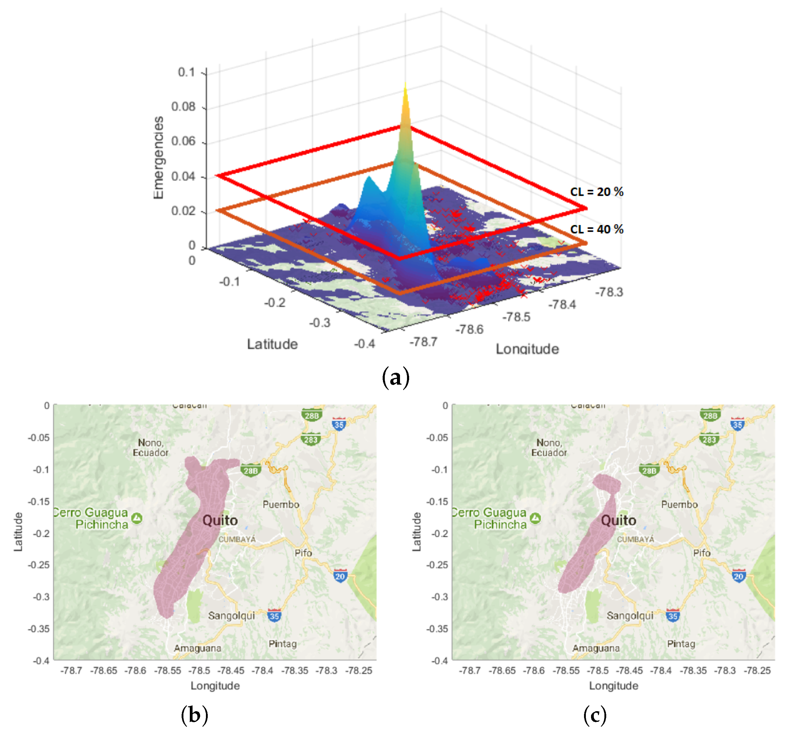
We can think of a Parzen window density estimation in our problem as a data interpolation technique that uses the emergency’s coordinates (i.e., latitude and longitude) to estimate a PDF [14]. This way, it allows us to graph a bidimensional surface with its higher amplitudes over the densest area of the represented events. We can define a CL, for example, 40% or 20%, as shown in Figure 3, and visualize the resulting contour where the plane P intercepts the PDF’s generated surface.
2.3.2. Short-Scale Adjustment of the Parzen Width
The previous subsection has described the use of Parzen windows to estimate the density function of events, for which we have to decide the value of the represented bandwidth. At a global observation scale, for example, the whole city, the method is robust for empirical methods of determining the bandwidth, as the samples contain a large number of events. For this reason, a heuristic criterion for bandwidth of about 0.01 can been used for exploration from a city representation scale. However, we would like to be able to work at different observation scales, in order to scrutinize further details in different regions of interest. For this purpose, we use two elements. First, a system of geographical representation yields the required flexibility in the support or our framework. Using Google Maps, we represented the emergencies on an adequate scale that allowed us to identify relevant details, such as the street names and sectors. Second, the option to work at different scales of observation depends on how the bandwidth is set, particularly if there are multimodalities. This last element is further developed next.
Botev et al. [17] proposed a purely data-driven algorithm to determine the bandwidth of Parzen windows, which avoids the use of any arbitrary reference rule and is particularly suitable for auto adjusting the bandwidth at different scales in our system. This method introduces an adaptive kernel density estimation (KDE) method based on the smoothing properties of the linear diffusion process. This method is known as Parzen kernel density deviation via diffusion (Parzen–KDD, for short). The use of Parzen–KDD allows for a better representation of Parzen windows in narrow scales and provides this with accuracy when locating small sets of events, as illustrated in Figure 4d.
We consider a KDE, given by
where is a Gaussian kernel with center location and scale , also known as the bandwidth.
In order to calculate the bandwidth in higher dimensions, it is necessary to know the asymptotically optimal squared bandwidth (), which is given by
where is a twice continuously differentiable function and for all . In order to estimate all for which and , the method uses established formulas for . The function is defined as
where is the viable plug-in estimator derived from
By solving Equation (15), it is possible to find and for the Gaussian kernel [17], and these have the form
Then, the squared bandwidth can be calculated with the following expressions:
These equations are the basis for the Parzen–KDD method.
3. Experiments and Results
The information saved in the DB used contained 121 variables, and these were obtained from the incoming alert calls converted into emergencies and attended by their corresponding PSAP, as shown in Figure 1. All the registered events were stored without any order or predefined pattern, but the geographical coordinates and several time references are available. To give an idea of the amount and quality of the available data in this DB, there were about 1,078,000 registered emergencies in the Quito PSAP only for 2014, and each event had valid information recorded in at least 50 of the 121 variables. These events were used as the basis for building and testing the system, providing us with the three described types of analytics and visualization, namely, temporal, geographical, and spatiotemporal.
3.1. Results of Temporal Analysis
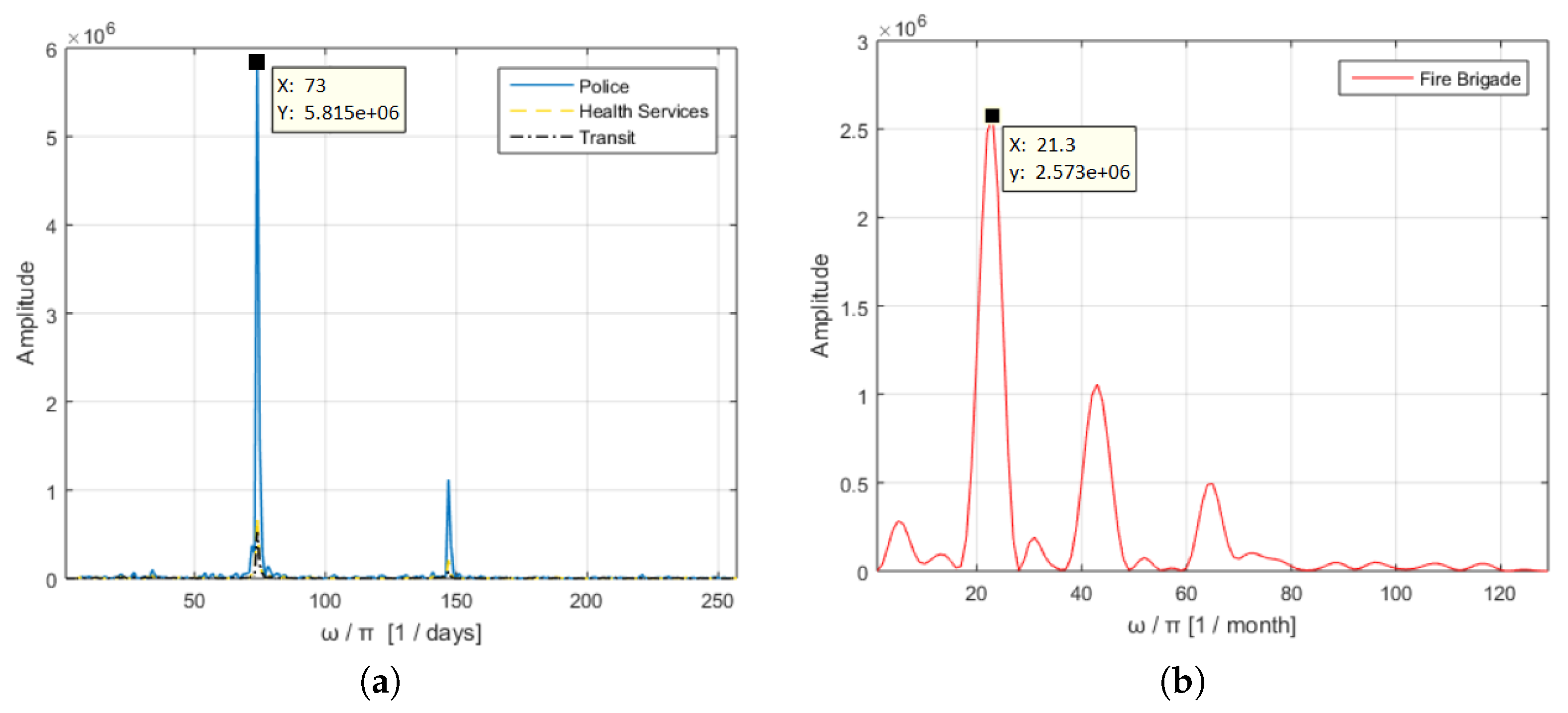
In the temporal domain, spectral analysis allowed us to recognize different periodical behaviors for each institution. By using the periodogram, we could determine or discard the near-periodical nature of these signals, which is a good indicator of seasonality in a data series [18]. Two examples of spectral analysis can be observed in Figure 5, where the fundamental period () of the analyzed signals could be obtained by taking into account the presence of a harmonic structure and then identifying its fundamental frequency. As seen in Figure 5a, there is a fundamental peak at the frequency corresponding to days, which means that the near-periodic pattern clearly repeated every week in the short-time periodic institution (STPI) services. On the other hand, Figure 5b shows a fundamental frequency peak corresponding to months, which clearly indicates the near-periodicity pattern of 1 year for the long-term periodic institution (LTPI) service.
According to the above observed temporal distributions of the registered events, we noted that the FRIs in Quito could be divided into three categories, as described next.
First, STPIs are those with a characteristic near-periodic behavior in short observation time intervals, that is, a week or a month. Police, health, and transit services can be included into this first category. Figure 6a illustrates the number of emergencies for these institutions over 2014, and Figure 6b details the month of March represented on a daily basis over the month. We can observe that Mondays usually exhibited the lowest number of events. The number of emergencies continued to increase during the other weekdays, and it reached the maximum values on weekends. Specifically, Saturday was most often the day when the peak of emergencies could be observed. This trend continued during the month and throughout the year. By comparing the plots of these three institutions, we can observe a similar behavior in terms of emergency peaks being coincident in similar days for this institution group.
Second, LTPIs are those with a near-periodic behavior during extended time intervals, in our case, a year. Figure 6c illustrates the emergencies corresponding to fire brigades over the years 2013 to 2016. In Figure 6d, four years are shown overlapping, and a characteristic pattern with a similar number of events can be observed during the first and last months of each year. In the third trimester, a dramatic increase in the number of emergencies can be seen, which was due to the summer season and its associated wildfire increase, according to [19]. The unusual peak of emergencies in April of 2016 corresponded to an earthquake of 5.9 degrees on the Ritcher scale that affected the country [20].
Finally, non-time periodic institutions (NTPIs) are those whose graphical representation or Fourier transform do not exhibit any periodic behavior, but rather they seem to be completely random and unrelated in terms of number of events. In our DB, RMS, military, and municipal services were included in this category. In Figure 6e we can see the emergencies that were attended during 2014 by these services, and Figure 6f shows March of 2014 represented with monthly and weekly scales.
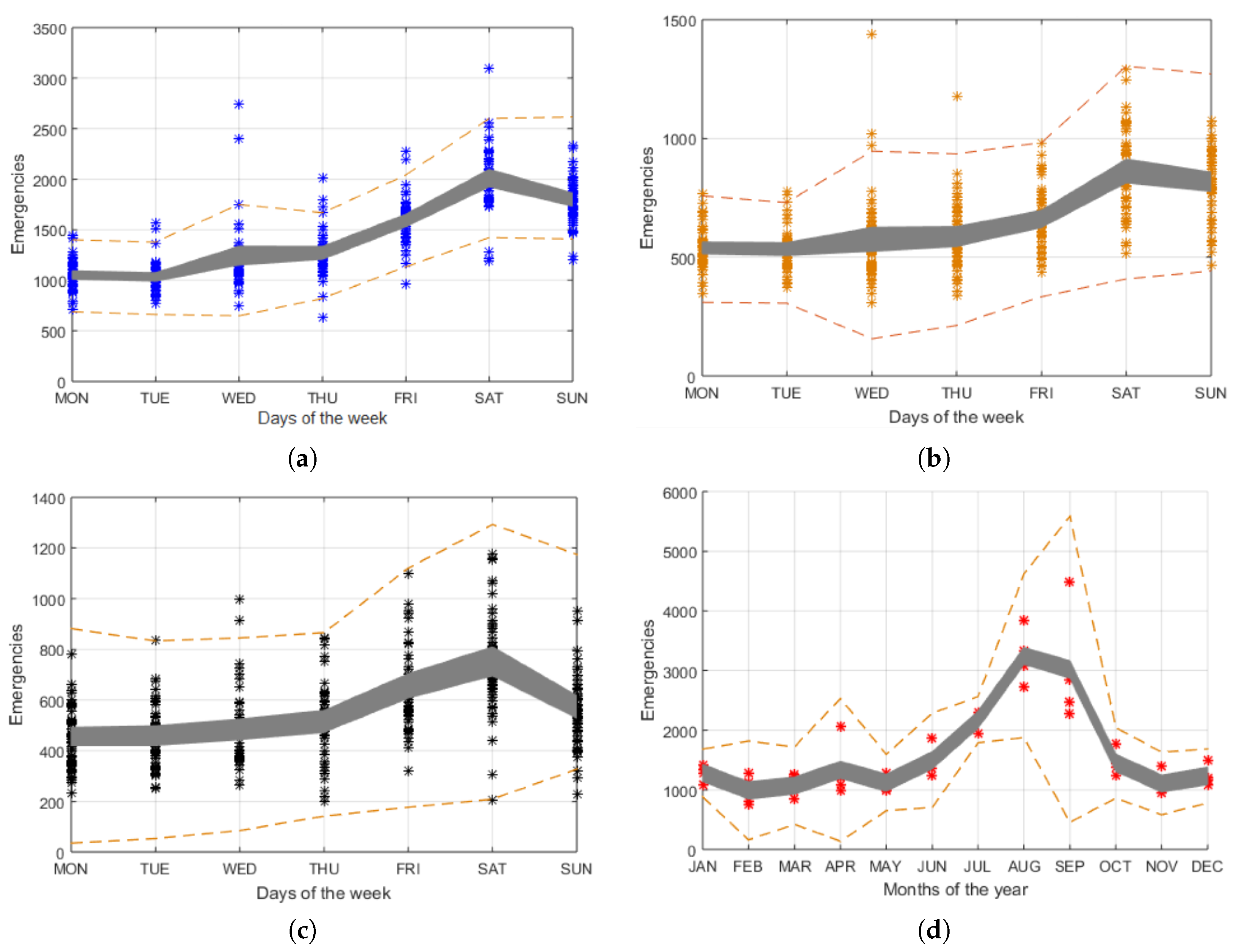
Given the near-periodicity present in both STPIs and LTPIs, it is useful to obtain their statistical temporal description, as given by the bootstrap CIs, trends, and outlier events (OEs). An OE is any observation outside of 1.5 times the interquartile range (IQR) over quartile Q3 and below quartile Q1 [21]. The time intervals considered for this analysis can be hourly, daily, weekly, monthly, or yearly. Emergencies recorded during 2014 were analyzed by overlapping the 52 weeks of the year. The results are depicted for police services in Figure 7a, for health services in Figure 7b, and for transit services in Figure 7c. The OEs are clearly seen as located outside of the dashed lines, and the CI is represented as the gray area. This temporal summary representation can be very helpful to support the manager analysis of the near-periodic behavior and to systematically analyze the OE, hence supporting the resource allocation by emergency managers of each institution. In all the cases, the CI confirmed this behavior in the analyzed institutions. For STPI, Saturdays registered the maximum peak of reported emergencies, and Mondays registered the lowest number. These three institutions had a similar weekly pattern. Figure 7d shows the characteristics of the LTPI, where 4 years were considered, from 2013 to 2016. The CI confirmed the behavior related with summer, forest fires and its yearly periodicity.
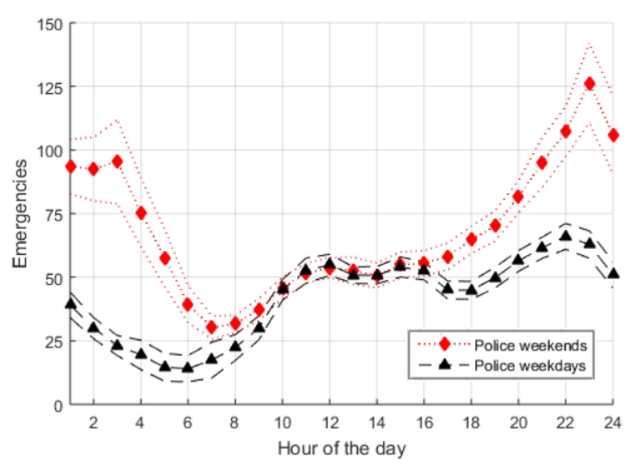
An hourly representation of the police events was further scrutinized, as seen in Figure 8, to show an example of short-term analysis. In this case, we overlapped the 365 days of the year, and these were divided into 24 h periods. This allowed us to identify the time interval of the day in which the number of events reached their maximum and minimum. We represented separately the yearly average of emergencies attended during weekdays versus weekends. In all the cases, we see that from midnight to 06h00, there was a dramatic decrement in the number of emergencies; during daylight hours, the number of events started to gradually rise, and from 18h00 to midnight the events reached their peak values. Once again, we see that the nights of weekends clearly registered the maximum number of attended emergencies. We note that, in this case, there was an overlap between 8 and 16 h, indicating that these hours were equally intense for all the days of the week in terms of police events.
3.2. Geographical and Spatiotemporal Analysis
As previously explained, two available variables in our DB were latitude and longitude of the emergency events. With this information, it was possible to geolocate these on a map for visual and numerical analysis of the geographical characterization of the FRIs under study. Although these types of geographical phenomena analyses and visualizations are being deeply studied [22,23], heatmap visualizations based on KDE approaches are one of the most widely applied solutions [24,25]. This popularity is due to their easy-to-modify character, in order to create efficient and scalable versions for different types of data, such as data streams [26,27] or big data [28,29,30]. For this reason, heatmap visualizations based on improved KDE methods have been used in a wide range of application fields, including traffic data visualization [31], emotional heatmaps [32], sentiment analysis [33,34,35], or human dynamics in social networks [36], among others. However, although level sets [23] and density pruning techniques [29] are studied for visualization, to the best of our knowledge, three-dimensional (3D) spatiotemporal visualization, as in Figure 9, has not been exploited to date, whereas it can be very useful to locate different spatiotemporal events in the same management panel.
In our system, the geographical representation was made over Google Maps, which can be readily handled with a publicly available function (plot_google_map.m) that uses an API (Application Programming Interface) developed by the same company [37]. The map coordinates were stored in the WGS84 reference system [38]. These geographical coordinates were used to search an image of a bidimensional map to place the emergencies as visible points, as observed in Figure 2b. The map scale could be settled to adapt the represented area according to the search criteria for the analyzed events.
Once the emergencies were placed over a reference map, we needed to identify the densest locations and represent these to create a heat map. With this purpose, a Parzen representation was applied, and some example results can be observed in Figure 4, where darker red areas correspond to a higher event density. In this case, a fixed bandwidth was used to yield a global (city-scale) view of emergencies in police, health, and transit services. We note that there is a noticeable similarity on the support for these three services, but the heat peaks are not always the same, as was the case for the time series peaks. For instance, police has a trimodal representation supported along the city, whereas health has a bimodal distribution, partially corresponding to that of the police, but with narrower main modes. On the other hand, transit events are distributed with strong multimodality, and their heat noticeably extends to the south-east, corresponding with one of the main roads that connects the city of Quito with the towns of Monjas, Conocoto and Sangolquí. In Figure 4d, we can observe Mariscal town on a short scale. In this case, by using Parzen–KDD, we could easily identify the points of higher concentration of police events. This accuracy is very useful when the responder institutions are planning the distribution of their units across the city for a faster response or to prevent incidents in the future.
As described in Section 2, the spatiotemporal analysis results from the combined analysis of spatial and temporal information of the emergencies registered in our DB. This combination allows us to better understand the occurrence of emergencies associated to each FRI. In other words, when we represent each confidence area in terms of 3D coordinates (latitude, longitude, and time), it is possible to obtain a useful visualization of the events [39]. In Figure 9, we represent the 95% confidence areas for each day in December 2014 (only 11 days are represented for ease of visualization on paper), corresponding to the police emergencies in the city of Quito. We note the temporal variations in the position of the slices with time, as well as the changes in shape and area. It is noteworthy to emphasize that this kind of variation remains hidden if we only scrutinize the temporal representations of the number of events.
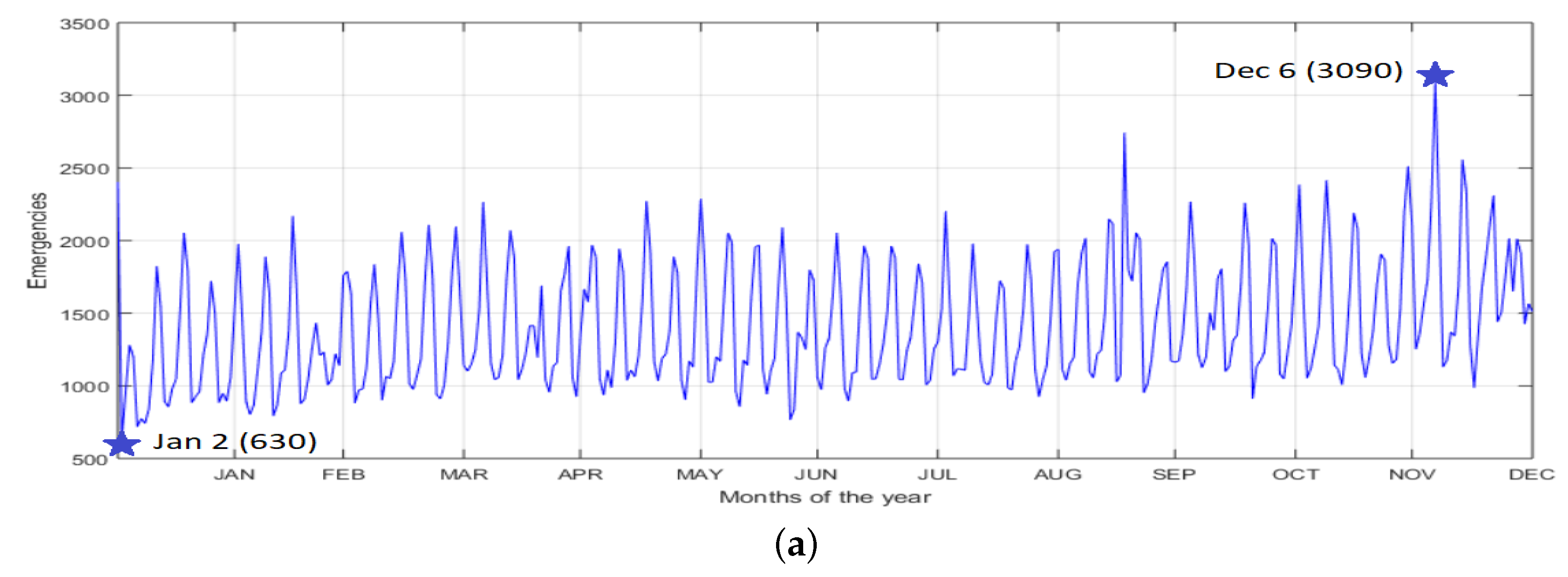
In order to further analyze STPIs and LTPIs, we compared the geographical Parzen estimation during the day of the maximum and minimum number of emergencies in 2014 and for each FRI. For the police service, the maximum peak of events was registered on Saturday 6 December, with 3090 emergencies, and the minimum was on Thursday 2 January, with 630 emergencies, as illustrated in Figure 10a. We note that this represents a noticeable number of emergencies, even for the minimum peak. The same figure depicts the Parzen distribution both in a red gradient over the map and its corresponding bidimensional PDF, for better visualization purposes. It is interesting to note that regions with intense activity for this service tended to be quite similar, as seen in the heat maps; however, their relative intensity was different over these days, which is more evident in the PDF representation. This points out that the modal regions with police activity were repetitive, whereas the intensity within these regions tended to be different over different time periods.
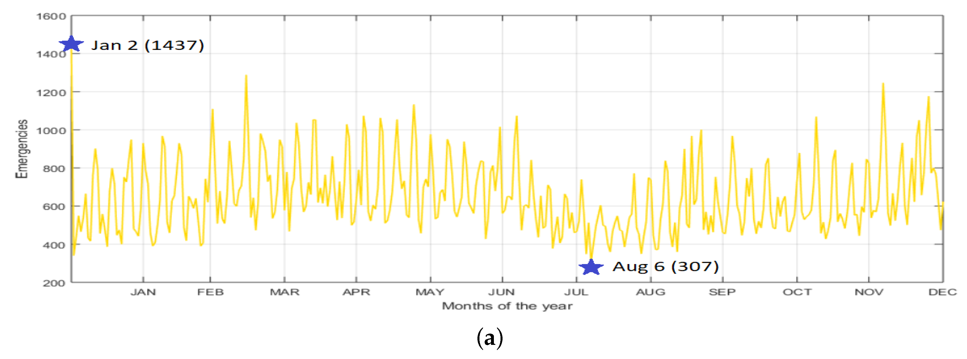
For health services, the maximum peak of events was registered on Wednesday 1 January, with 1437 emergencies, and the minimum was on Wednesday 6 August, with 307 emergencies. Figure 11 shows a similar representation for these, making evident that in this case the dynamics were different, as far as some modal regions were repeated (in the south and along roads to the east and south-east), but other modal areas were very different, which was made more evident in the PDF representations. Therefore, health emergencies were more variable in terms of their geographical support, and not only in the intensity of events.
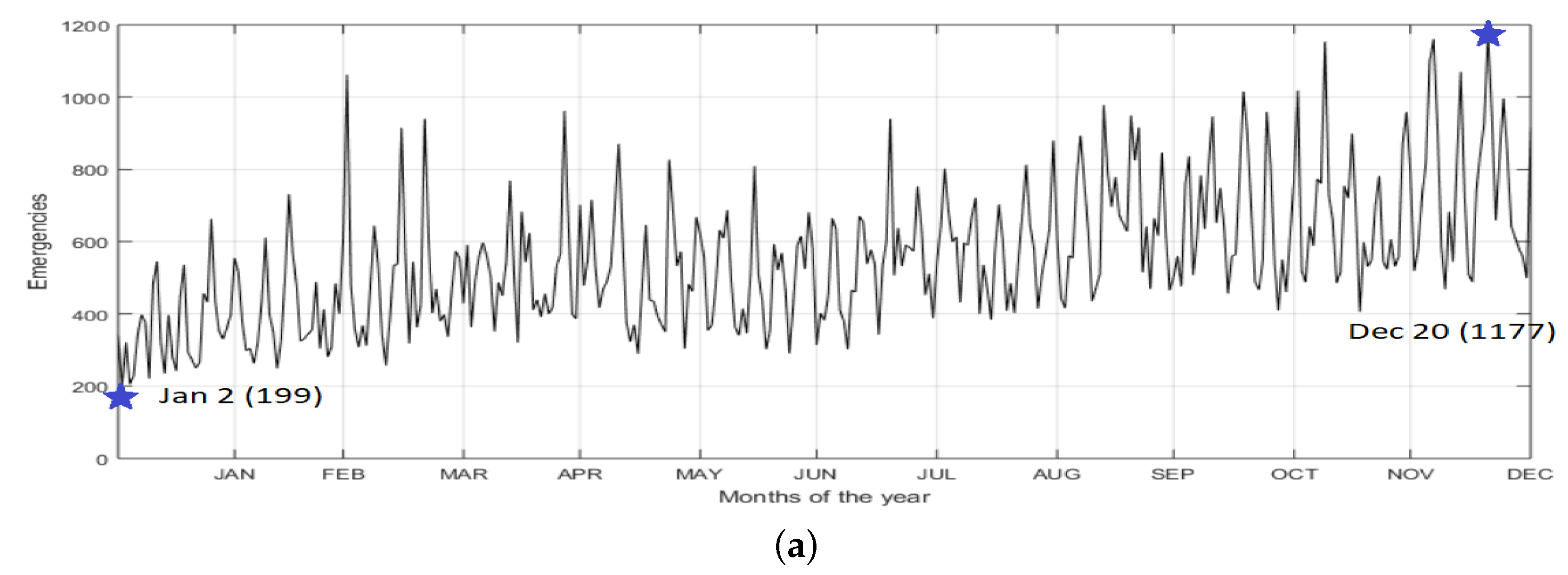
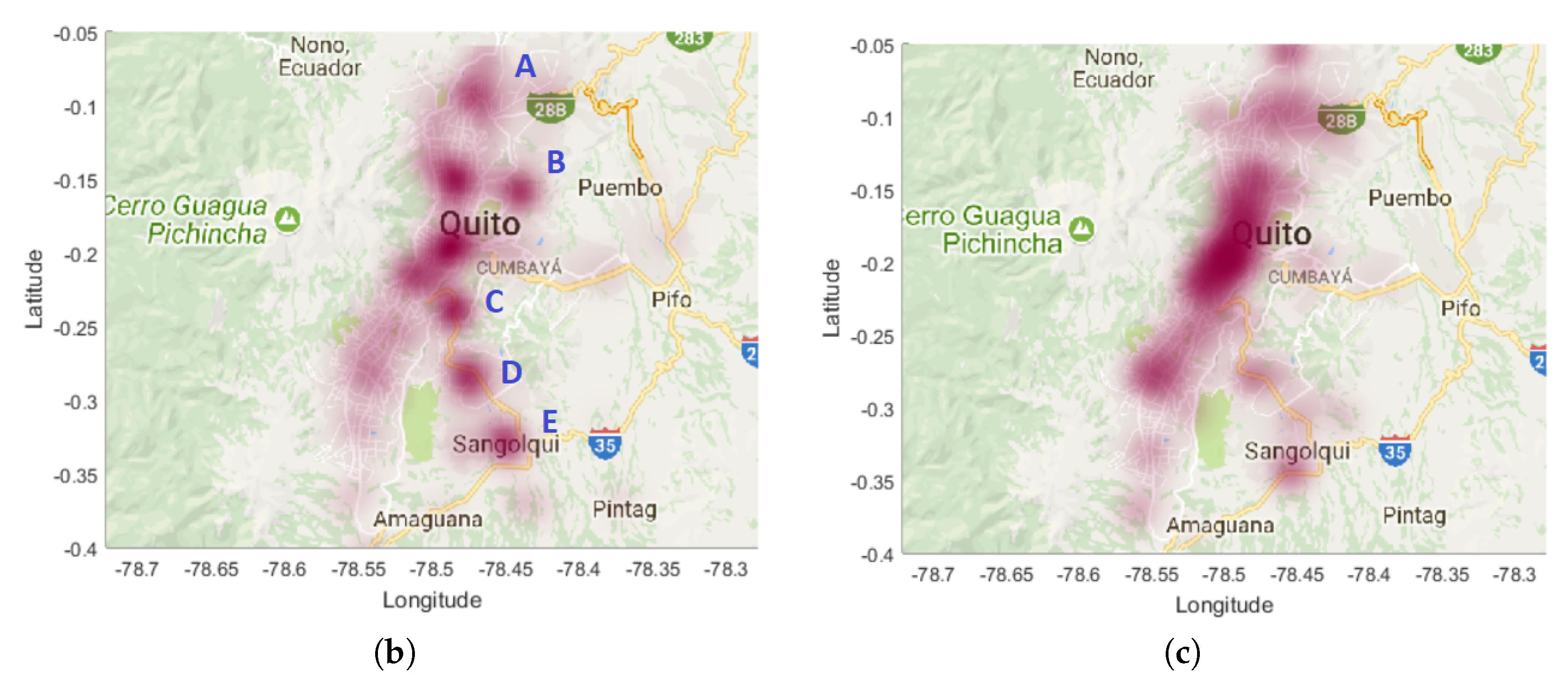
For transit services, the maximum peak was on Saturday 20 December, with 1177 emergencies, and the minimum was on Thursday 2 January, with 199 emergencies, as Figure 12a shows. On weekends, transit emergencies were distributed in a wider area that included sectors and small towns around Quito, compared to the weekdays. The visible distribution modes allowed us to identify concentrations in Carcelen (A), Tanda (B), Luluncoto (C), Conocoto (D), and Sangolquí (E), which correspond to the city periphery (see Figure 12b). During weekdays, transit emergencies were mainly concentrated in the urban area of the city, as clearly seen in Figure 12c.
For fire brigades, the maximum peak of events was registered on Sunday 21 September, with 1618 emergencies, and the minimum was on Monday 27 January, with 36 emergencies, as is illustrated in Figure 13a. In Figure 13b, it is easy to identify two main event concentrations located in Carretas (A) and Tumbaco (B) towns. Figure 13c shows the 3D Parzen distribution over the map. These peaks of events are highlighted as the most visible. Finally, Figure 13d,e shows Parzen–KDD representations for the maximum peaks registered. Carretas (A) and Tumbaco (B) emergencies can be observed in this order. It can be seen that the geographical representation was often found to be very useful to accurately locate the emergencies reported to a PSAP and similar surveillance systems [19,40].
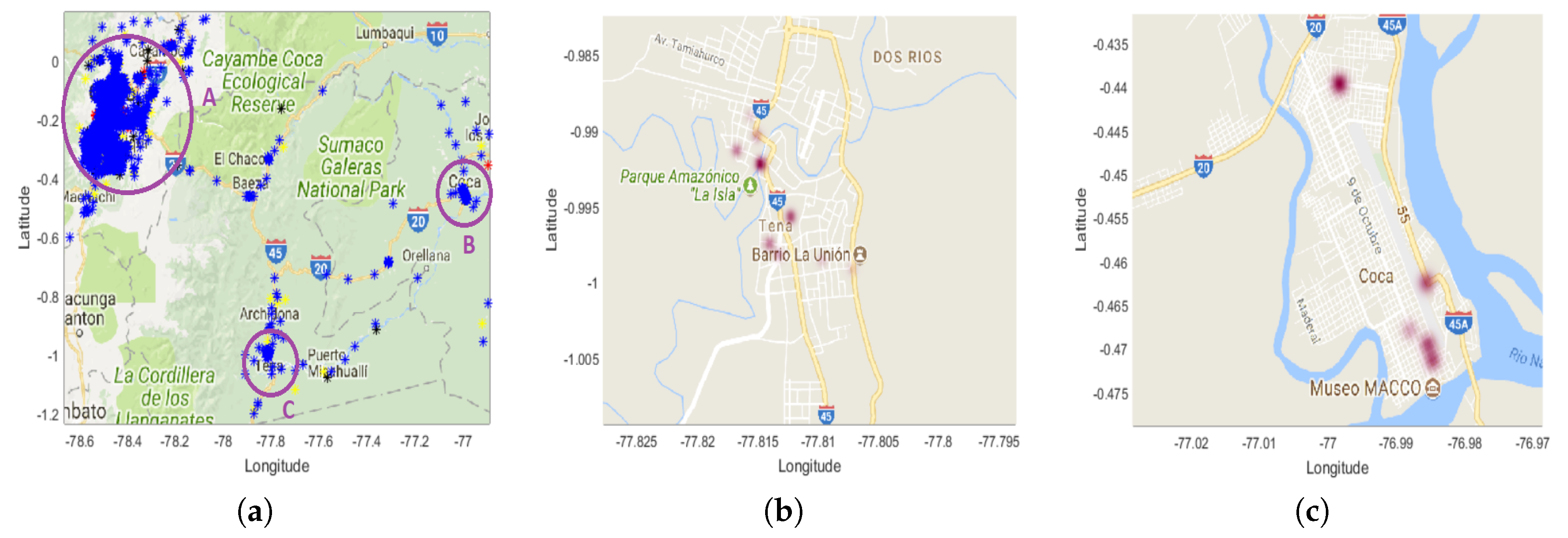
The PSAP of Quito covers three provinces, namely, Pichincha, Napo, and Orellana, and their respective capitals are Quito (2,644,145 inhabitants), Tena (74,158 inhabitants), and El Coca (88,106 inhabitants). The largest number of emergencies were concentrated in the Quito metropolitan district and its near towns. Their combined population is close to the 3 million persons. Napo and Orellana are two of the six Amazonic provinces of the country. The Amazonic region represents almost the 45% of the total surface of the country; less than 5% of the Ecuadorian population are living in it. This nonuniform demographic distribution explains the lower density of emergencies registered in the other two provinces when we compare these with Quito. In Figure 14a, we can observe the cities of (A) Quito, (B) Napo, and (C) El Coca. It is easy to note the concentration of events registered along January 2014. Figure 14b,c illustrates the cities of Tena and El Coca, respectively. In these cities, most of events were registered in the urban parts. The surrounding territory is essentially tropical jungle with prevailing high temperatures and humidity, very low highways, and a number of protected areas and national parks. If we add this to the low density of the population, we can easily explain the low number of events registered in both provinces compared with Quito. Nevertheless, this represents highly different event dynamics in these regions, which also needs to be adequately characterized in time and space and in statistical terms, for its adequate management.
4. Discussion and Conclusions
The unprecedented growth in the amount of data related with 911 events has increased the need for agile processing and visualization. When large amounts of data are available, even simple statistical, temporal, and geographical descriptions are necessary and strongly informative. In this work, we propose a system for temporal analysis, including seasonal representations and nonparametric CIs, together with spatial representations, including heat maps, in terms of Parzen estimations. In the case study of 911 events in Quito, temporal analysis allowed us to divide the FRIs into three groups according to the periodicity of the registered events, namely, STPIs, LTPIs, and NTPIs. More than 1 million emergencies were analyzed for this research in terms of relatively simple statistical descriptions. For periodically behaved institutions, seasonal patterns were identified separately from trends and atypical events. From the geographical-analysis point of view, the emergencies could be readily seen over a referenced Google Map, and their spatial dynamics could be observed and quantified; moreover, FRIs could be scrutinized from different scales.
The proposed system can be used to provide 911 managers with statistical, spatial, and temporal analysis of the emergencies registered in a PSAP. The temporal and geographical visualization is a necessary tool, but we would like to stress that the proposed system is not just a visualization tool. Statistical processing provides us with powerful analysis tools and relevant information, which cannot fully be extracted from raw data, as in Figure 2. The use of bootstrap resampling and Parzen windowing is quite an operative statistical approach to these data, as far as these nonparametric methods are easy to use in order to deal with statistical tests and density estimations under conditions for which the underlying statistical distributions cannot be assumed as known. The efficient management of resources requires an agile and natural time–space representation supporting system and an adequate statistical analysis to convert the set of events into meaningful and solidly estimated dynamics. Whereas some of the results presented here can seem trivial (i.e., a larger number of events in the weekend), a solid quantification is the basis for establishing resource allocation. From this point, we can move now towards the design of systems used for resource allocation, by combining the resource information with the quantified data model, as well as towards more advanced and improved estimation and data processing tools. For instance, more advanced data analysis algorithms, prediction systems, or parametric statistical analysis can now be pursued. The role from the other recorded variables in the DB certainly remains to be exploited. Moreover, data quality considerations are also to be taken into account, as is usual in problems based on storing large amounts of data.
In fact, by using the information obtained with the developed tool, the institutions do not depend only on the empirical experience of the dispatchers. Usually, this kind of experience takes several months to be learned for people that work in the dispatching area. The spatial dynamics for each FRI are even more complicated in terms of being abstracted by the dispatchers. We note that the present work does not only present a temporal representation of the emergencies, but also a geographical representation in which “hot points” can be identified. Hence, through our proposal, the occurrence of different emergency types at different locations can be characterized, hence allowing the saving of time when resources are preallocated according to the type and approximate number of expected events. Moreover, economical resources can be saved when units for emergency attendance are not constantly moved or travel only short distances. This is also very relevant when an opportune response may save lives as a result of a technical planning method. For instance, knowing the concentration of crimes against the property, police units may be placed in fixed or mobile stations close to these hot areas, which allows for a fast response if an emergency is reported. This will definitively increase the security of these zones, and this is also considered as a dissuasive element to illicit actions.
Future work includes the detailed analysis of specific emergency types attended by each institution and its statistical behavior with time. All of this is oriented to planning the distribution of resources on territory for an efficient future response to the occurrence of the studied emergencies, for example, the occurrence of car accidents during holidays on a specific highway. Knowing the distribution of these events, it will be possible to obtain the road safety risk evaluation [41] and plan the location of resources for the next periods of time, looking to minimize the response time or, in the best case, preventing the occurrence of the referred events.
Acknowledgments
This work was partly supported by the Universidad de las Fuerzas Armadas ESPE under Grant 2015-PIC-004, by Research Grants PRINCIPIAS, FINALE, and KERMES (TEC2013-48439-C4-1-R, TEC2016-75161-C2-1-R, and TEC2016-81900-REDT) from the Spanish Government and by PRICAM (S2013/ ICE-2933) from Comunidad de Madrid, Spain. The authors thank ECU 911 of Ecuador for providing the event database.
Author Contributions
Danilo Corral-De-Witt and Enrique V. Carrera designed and implemented the database, conducted the experiments, organized and wrote the paper, and performed the analysis of the experimental results. José Luis Rojo-Álvarez, Sergio Muñoz-Romero, and Enrique V. Carrera collaborated and reviewed the writing of some sections of the manuscript, as well as analyzed some experimental charts. Sergio Muñoz-Romero collaborated in the code of the experiments.
Conflicts of Interest
The authors declare no conflict of interest.
References
- Marshall, R.; Schulzrinne, H. Requirements for Emergency Context Resolution with Internet Technologies; Securities and Exchange Commission: Washington, DC, USA, 2008.
- Swales, S.C.; Maloney, J.E.; Stevenson, J.O. Locating mobile phones and the US wireless E-911 mandate. In Proceedings of the Novel Methods of Location and Tracking of Cellular Mobiles and Their System Applications, London, UK, 17 May 1999; pp. 2/1–2/6. [Google Scholar]
- Reed, J.H.; Krizman, K.J.; Woerner, B.D.; Rappaport, T.S. An Overview of the Challenges and Progress in Meeting the E-911. IEEE Commun. Mag. 1998, 36, 30–37. [Google Scholar] [CrossRef]
- Seeman, E.; Holloway, J.E. Next generation 911: when technology drives public policy. Int. J. Bus. Contin. Risk Manag. 2013, 4, 23–35. [Google Scholar] [CrossRef]
- Schabenberger, O.; Gotway, C.A. Statistical Methods for Spatial Data Analysis; CRC Press: Boca Raton, FL, USA, 2017; pp. 1–6. [Google Scholar]
- Wan-Jo, B.; Asad-Khan, R.M. An Event Reporting and Early-Warning Safety System Based on the Internet of Things for Underground Coal Mines: A Case Study. Appl. Sci. 2017, 7, 925. [Google Scholar] [CrossRef]
- Segura-García, J.; Pérez-Solano, J.J.; Cobos-Serrano, M.; Navarro-Camba, E.A.; Felici-Castell, S.; Soriano-Asensi, A.; Montes-Suay, F. Spatial Statistical Analysis of Urban Noise Data from a WASN Gathered by an IoT System: Application to a Small City. Appl. Sci. 2016, 6, 380. [Google Scholar] [CrossRef]
- Hong, Y.; Bonhomme, C.; Soheilian, B.; Chebbo, G. Effects of Using Different Sources of Remote Sensing and Geographic Information System Data on Urban Stormwater 2D–1D Modeling. Appl. Sci. 2017, 7, 904. [Google Scholar] [CrossRef]
- Jennex, M.E. Modeling emergency response systems. In Proceedings of the 40th Annual Hawaii International Conference on System Sciences, Waikoloa, HI, USA, 3–6 January 2007; Available online: http://ieeexplore.ieee.org/abstract/document/4076412/authors (accessed on 29 January 2018).
- ECU911. Estadisticas. Available online: http://www.ecu911.gob.ec/estadisticas/ (accessed on 28 July 2017).
- Hassani, S. Mathematical Methods: For Students of Physics and Related Fields; Springer Science & Business Media: New York, NY, USA, 2008; Volume 720. [Google Scholar]
- Efron, B.; Tibshirani, R.J. An Introduction to the Bootstrap; CRC Press: Boca Raton, FL, USA, 1994. [Google Scholar]
- Alonso-Atienza, F.; Rojo-Álvarez, J.L.; Rosado-Muñoz, A.; Vinagre, J.J.; García-Alberola, A.; Camps-Valls, G. Feature selection using support vector machines and bootstrap methods for ventricular fibrillation detection. Expert Syst. Appl. 2012, 39, 1956–1967. [Google Scholar] [CrossRef]
- Parzen, E. On estimation of a probability density function and mode. Ann. Math. Statist. 1962, 33, 1065–1076. [Google Scholar] [CrossRef]
- Yeung, D.Y.; Chow, C. Parzen-window network intrusion detectors. In Proceedings of the 16th International Conference on Pattern Recognition, Quebec, QC, Canada, 11–15 August 2002; Volume 4, pp. 385–388. [Google Scholar]
- Figuera, C.; Mora-Jimenez, I.; Guerrero-Curieses, A.; Rojo-Alvarez, J.; Everss, E.; Wilby, M.; Ramos-Lopez, J. Nonparametric model comparison and uncertainty evaluation for signal strength indoor location. IEEE Trans. Mob. Comput. 2009, 8, 1250–1264. [Google Scholar] [CrossRef]
- Botev, Z.I.; Grotowski, J.F.; Kroese, D.P. Kernel density estimation via diffusion. Ann. Stat. 2010, 38, 2916–2957. [Google Scholar] [CrossRef] [Green Version]
- Stoica, P.; Moses, R.L. Spectral Analysis of Signals; Pearson Prentice Hall: Upper Saddle River, NJ, USA, 2005; Volume 452, pp. 25–26. [Google Scholar]
- Martin, J.; Hillen, T. The spotting distribution of wildfires. Appl. Sci. 2016, 6, 177. [Google Scholar] [CrossRef]
- Medina, A.R.; Oterino, B.; Belen, M.; Escribano, G.; Miguel, J.; Cárdenas, P.; Aníbal, H.; Aníbal, H.; Roberto, A.; Santiago, T.; et al. Aceleraciones registradas y calculadas del sismo del 12 de agosto de 2014 en Quito. Ciencia 2014, 16, 139–153. [Google Scholar]
- Walfish, S. A review of statistical outlier methods. Pharm. Technol. 2006, 30, 82. [Google Scholar]
- Correll, M.; Heer, J. Surprise! Bayesian Weighting for De-Biasing Thematic Maps. IEEE Trans. Vis. Comput. Graph. 2017, 23, 651–660. [Google Scholar] [CrossRef] [PubMed]
- Chen, Y.C.; Genovese, C.R.; Wasserman, L. Density Level Sets: Asymptotics, Inference, and Visualization. J. Am. Stati. Assoc. 2017, 1–13. [Google Scholar] [CrossRef]
- Wang, F. Visual Analytics Methods for Exploring Geographically Networked Phenomena. Ph.D Thesis, Arizona State University, Tempe, AZ, USA, 2017. [Google Scholar]
- Spencer, C.; Yakymchuk, C.; Ghaznavi, M. Visualising data distributions with kernel density estimation and reduced chi-squared statistic. Geosci. Front. 2017, 8, 1247–1252. [Google Scholar] [CrossRef]
- Qahtan, A.; Wang, S.; Zhang, X. KDE-Track: An Efficient Dynamic Density Estimator for Data Streams. IEEE Trans. Knowl. Data Eng. 2017, 29, 642–655. [Google Scholar] [CrossRef]
- Li, C.; Baciu, G.; Yu, H. StreamMap: Smooth Dynamic Visualization of High-Density Streaming Points. IEEE Trans. Vis. Comput. Graph. 2017. [Google Scholar] [CrossRef] [PubMed]
- Perrot, A.; Bourqui, R.; Hanusse, N.; Lalanne, F.; Auber, D. Large interactive visualization of density functions on big data infrastructure. In Proceedings of the 2015 IEEE 5th Symposium on Large Data Analysis and Visualization (LDAV), Chicago, IL, USA, 25–26 October 2015; pp. 99–106. [Google Scholar]
- Gan, E.; Bailis, P. Scalable Kernel Density Classification via Threshold-Based Pruning. In Proceedings of the SIGMOD 17 2017 ACM International Conference on Management of Data; ACM: New York, NY, USA, 2017; pp. 945–959. [Google Scholar]
- Zheng, Y.; Ou, Y.; Lex, A.; Phillips, J.M. Visualization of Big Spatial Data using Coresets for Kernel Density Estimates. arXiv, 2017; arXiv:1709.04453. [Google Scholar]
- Chen, W.; Guo, F.; Wang, F.Y. A Survey of Traffic Data Visualization. IEEE Trans. Intell. Transp. Syst. 2015, 16, 2970–2984. [Google Scholar] [CrossRef]
- Shook, E.; Leetaru, K.; Cao, G.; Padmanabhan, A.; Wang, S. Happy or not: Generating topic-based emotional heatmaps for Culturomics using CyberGIS. In Proceedings of the 2012 IEEE 8th International Conference on E-Science, Chicago, IL, USA, 8–12 October 2012; pp. 1–6. [Google Scholar]
- Kucher, K.; Paradis, C.; Kerren, A. The State of the Art in Sentiment Visualization. Comput. Graph. Forum 2017. [Google Scholar] [CrossRef]
- Beigi, G.; Hu, X.; Maciejewski, R.; Liu, H. An Overview of Sentiment Analysis in Social Media and Its Applications in Disaster Relief. In Sentiment Analysis and Ontology Engineering: An Environment of Computational Intelligence; Pedrycz, W., Chen, S.M., Eds.; Springer International Publishing: Cham, Switzerland, 2016; pp. 313–340. [Google Scholar]
- Lu, Y.; Hu, X.; Wang, F.; Kumar, S.; Liu, H.; Maciejewski, R. Visualizing Social Media Sentiment in Disaster Scenarios. In Proceedings of the 24th International Conference on World Wide Web; ACM: New York, NY, USA, 2015; pp. 1211–1215. [Google Scholar]
- Cuenca-Jara, J.; Terroso-Saenz, F.; Valdes-Vela, M.; Skarmeta, A.F. Fuzzy Modelling for Human Dynamics Based on Online Social Networks. Sensors 2017, 17, 1949. [Google Scholar] [CrossRef] [PubMed]
- Google.com. Google Maps API. Available online: https://developers.google.com/maps/documentation/embed/start (accessed on 28 July 2017).
- Snay, R.A.; Soler, T. Modern terrestrial reference systems part 3: WGS 84 and ITRS. Prof. Surv. 2000, 203, 1–3. [Google Scholar]
- Jasso, H.; Fountain, T.; Baru, C.; Hodgkiss, W.; Reich, D.; Warner, K. Spatiotemporal analysis of 9-1-1 call stream data. In Proceedings of the 2006 International Conference on Digital Government Research, San Diego, CA, USA, 21–24 May 2006; pp. 21–22. [Google Scholar]
- Gazquez, J.A.; Garcia, R.M.; Castellano, N.N.; Fernandez-Ros, M.; Perea-Moreno, A.J.; Manzano-Agugliaro, F. Applied Engineering Using Schumann Resonance for Earthquakes Monitoring. Appl. Sci. 2017, 7, 1113. [Google Scholar] [CrossRef]
- Shah, S.A.R.; Brijs, T.; Ahmad, N.; Pirdavani, A.; Shen, Y.; Basheer, M.A. Road Safety Risk Evaluation Using GIS-Based Data Envelopment Analysis—Artificial Neural Networks Approach. Appl. Sci. 2017, 7, 886. [Google Scholar] [CrossRef]
Figure 1.
Overview of a public safety answering point (PSAP): (a) basic operation; (b) proposed model. DB: database; FRIs: first response institutions.
Figure 1.
Overview of a public safety answering point (PSAP): (a) basic operation; (b) proposed model. DB: database; FRIs: first response institutions.
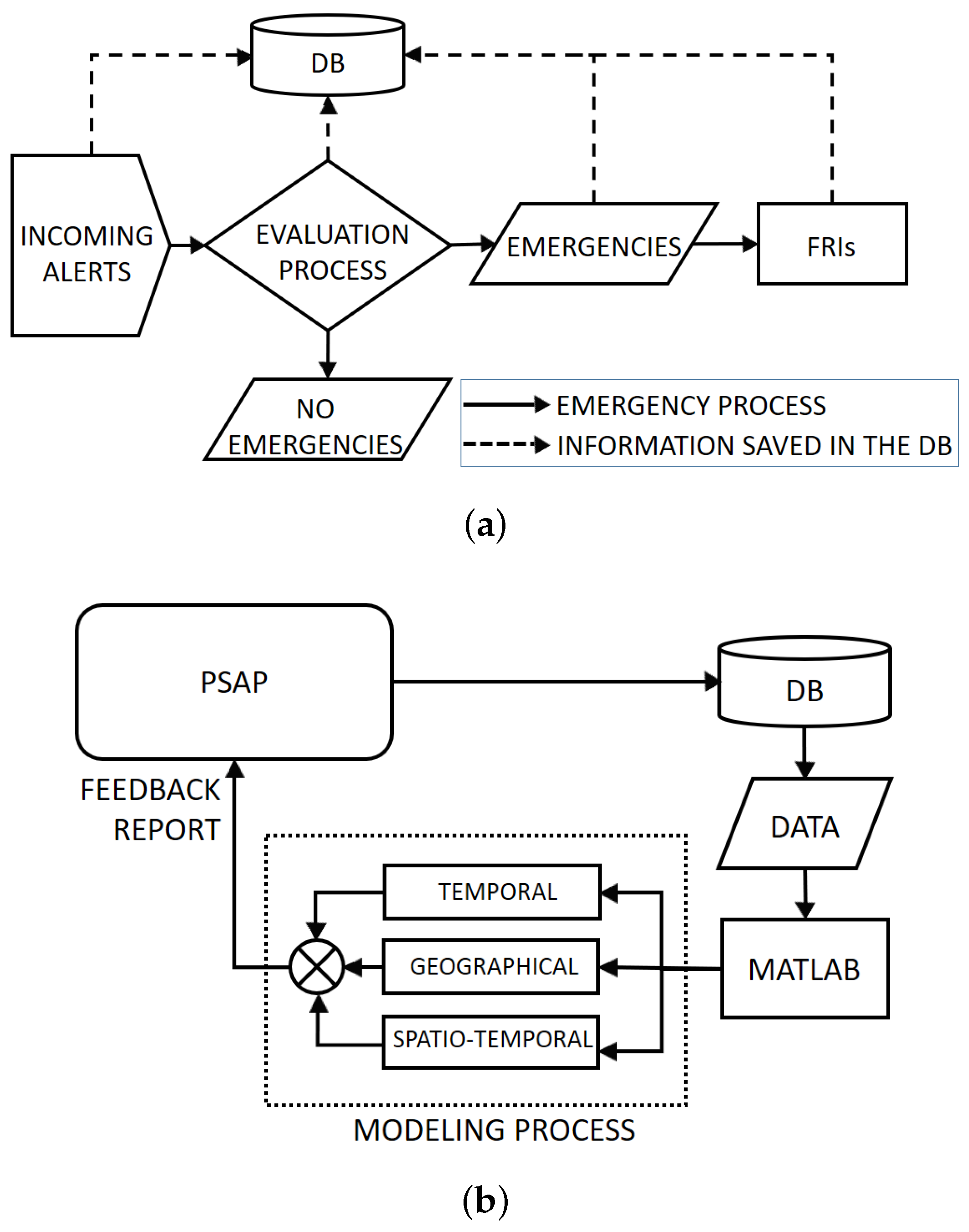
Figure 2.
Emergencies registered during January, 2014. Number of events as a function of time during the first and third weeks (a,c); grouped by hours, and their scatterplots (b,d).
Figure 2.
Emergencies registered during January, 2014. Number of events as a function of time during the first and third weeks (a,c); grouped by hours, and their scatterplots (b,d).

Figure 3.
A confidence level (CL) visualization shows the contour that results from the intersection of the Parzen solid representation and the settled horizontal plane, as seen in (a); (b,c) contour visualization for CL = 40% and CL = 20%.
Figure 3.
A confidence level (CL) visualization shows the contour that results from the intersection of the Parzen solid representation and the settled horizontal plane, as seen in (a); (b,c) contour visualization for CL = 40% and CL = 20%.

Figure 4.
Overview of emergency events in the city of Quito during 6 December, as represented by their Parzen estimation for (a) police; (b) health; and (c) transit services, using a global width for all of these; (d) representation of event density using Parzen kernel density deviation via diffusion (KDD) for police on a short scale over Mariscal town.
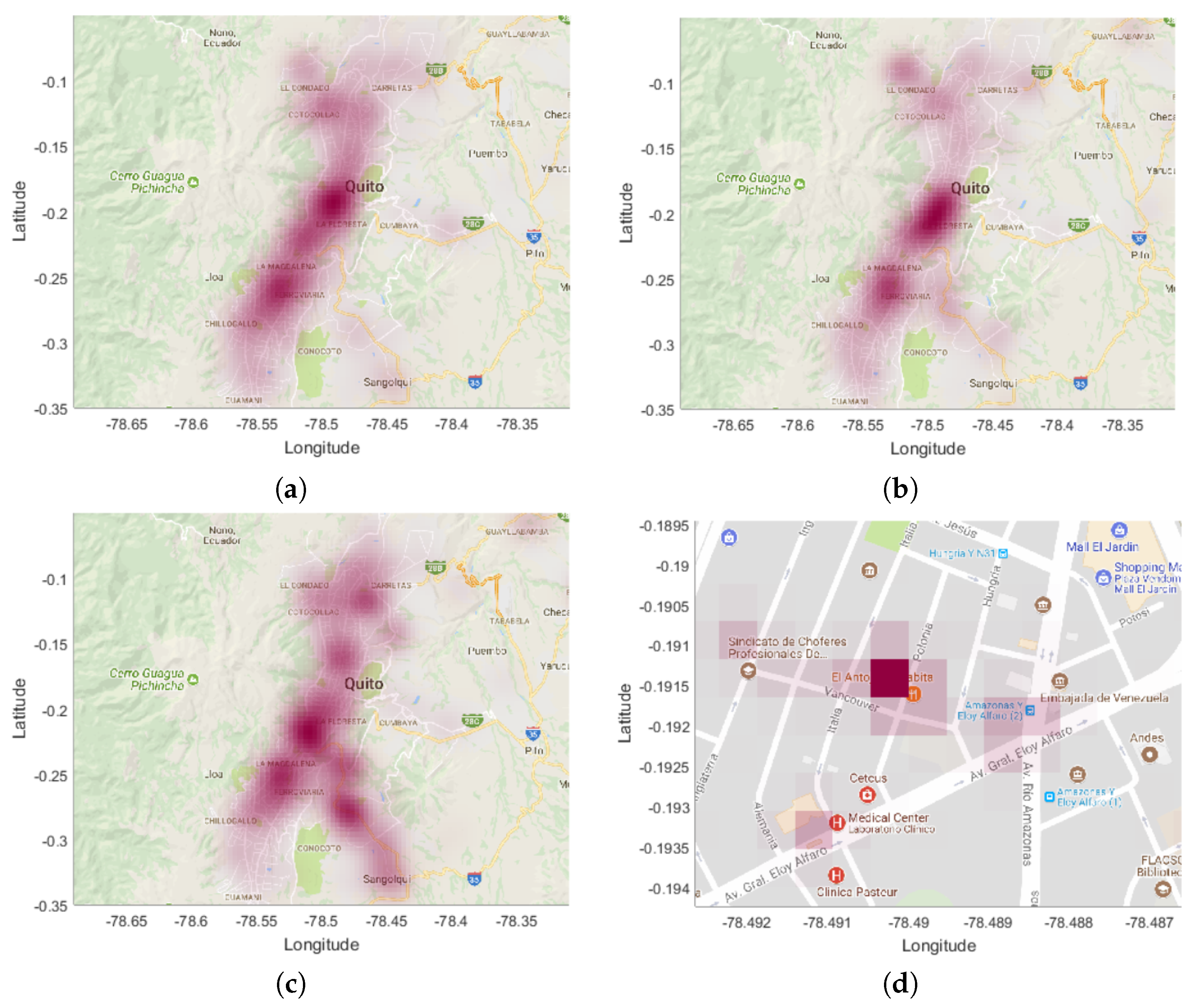
Figure 5.
Spectral analysis of short-time periodic institution (STPI) (a) and long-term periodic institution (LTPI) (b) examples. The narrowband spectrum in both cases and the clear presence of harmonics highlight the periodic and seasonal character of these institutions.
Figure 5.
Spectral analysis of short-time periodic institution (STPI) (a) and long-term periodic institution (LTPI) (b) examples. The narrowband spectrum in both cases and the clear presence of harmonics highlight the periodic and seasonal character of these institutions.

Figure 6.
Emergencies registered during 2014, grouped by temporal visual trends: (a,b) police, health, and transit services; (c,d) fire brigade; (e,f) risk management secretary (RMS), military, and municipal services.
Figure 6.
Emergencies registered during 2014, grouped by temporal visual trends: (a,b) police, health, and transit services; (c,d) fire brigade; (e,f) risk management secretary (RMS), military, and municipal services.
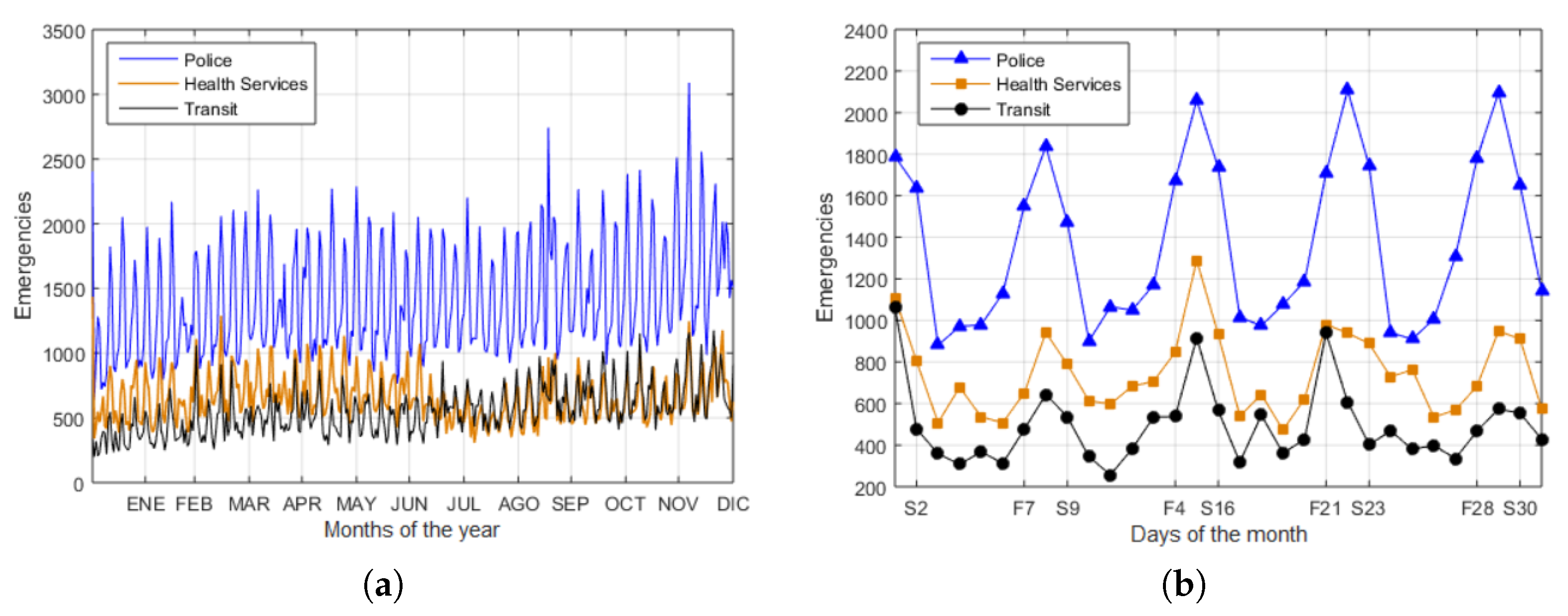
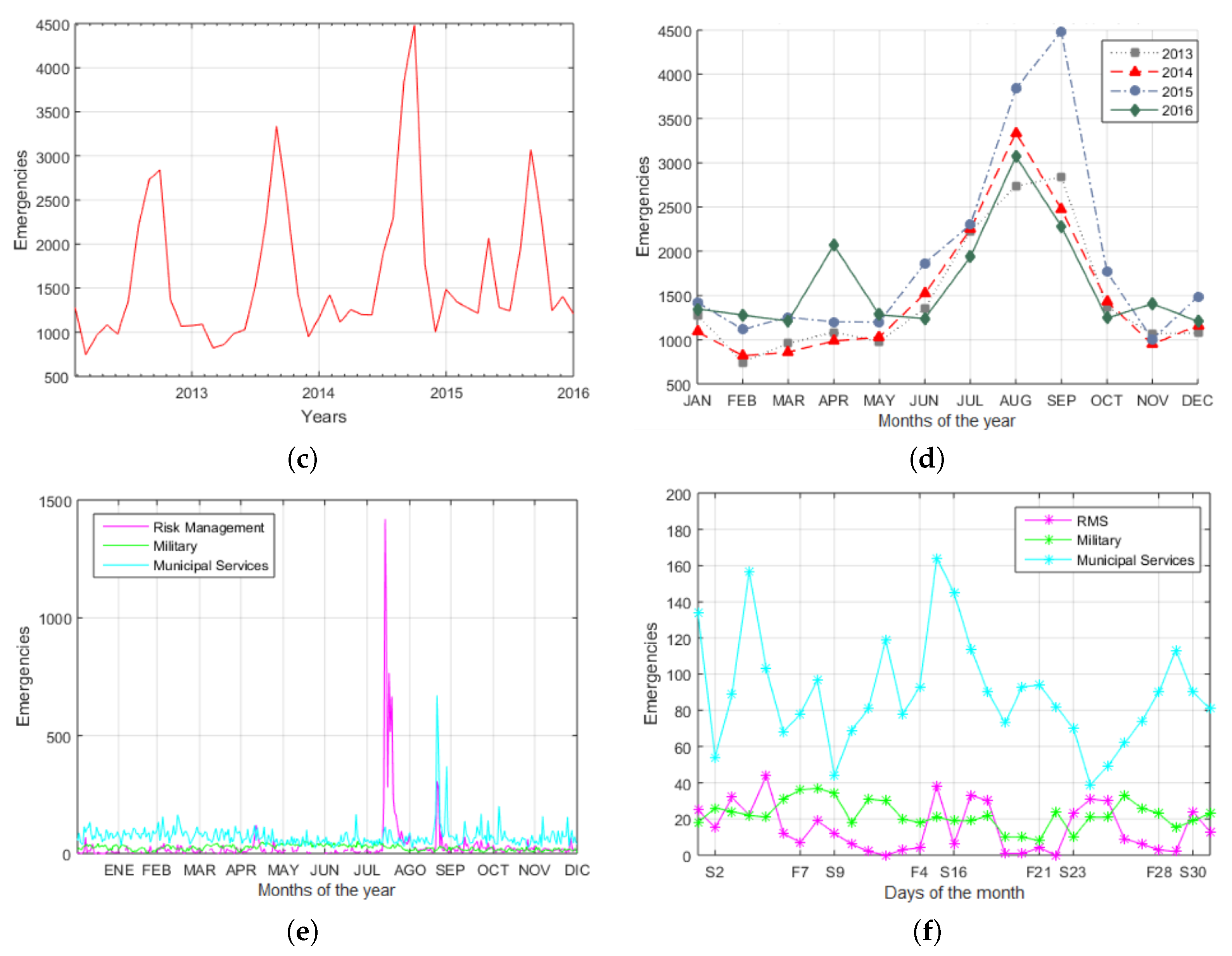
Figure 7.
Temporal representation of the confidence interval (CI) of events during 2014, for police (a); health (b); and transit (c) services; as well as fire brigade events over 4 years, from 2013 to 2016 (d). Dashed lines are the criterion used to identify the OE, and gray areas are used to characterize the repeating patterns and subsequent resource allocation by managers.

Figure 8.
Police emergencies by hours during 2014. Average of the 365 days of the year and their confidence intervals (CIs) are represented. Weekdays versus weekends emergencies can be seen with their variations.
Figure 8.
Police emergencies by hours during 2014. Average of the 365 days of the year and their confidence intervals (CIs) are represented. Weekdays versus weekends emergencies can be seen with their variations.

Figure 9.
Spatiotemporal emergency slices for police during December (only 11 nonconsecutive days are illustrated for better visualization on page). It is easy to notice with this representation the variations in the geographical concentration of events during the month and its concentration over different regions of the city.
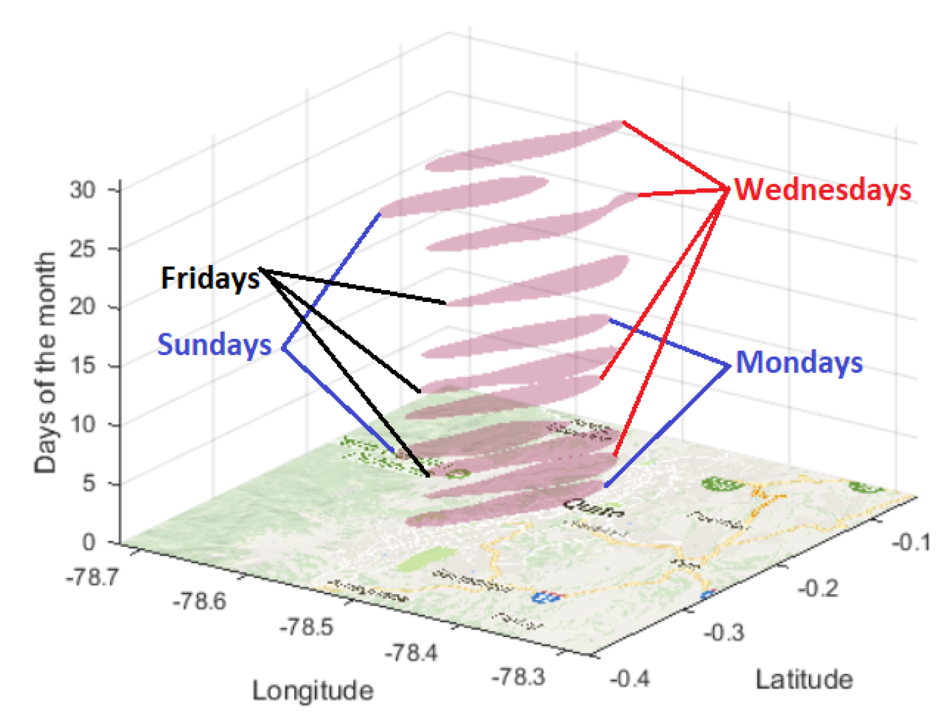
Figure 10.
Analysis of police emergencies. (a) Events during 2014, with maximum and minimum peaks; (b,c) Parzen distribution in red gradient over the map and bidimensional probability density function (PDF) representation for maximum peak on December 6; (d,e) The same for minimum peak on 2 January.
Figure 10.
Analysis of police emergencies. (a) Events during 2014, with maximum and minimum peaks; (b,c) Parzen distribution in red gradient over the map and bidimensional probability density function (PDF) representation for maximum peak on December 6; (d,e) The same for minimum peak on 2 January.

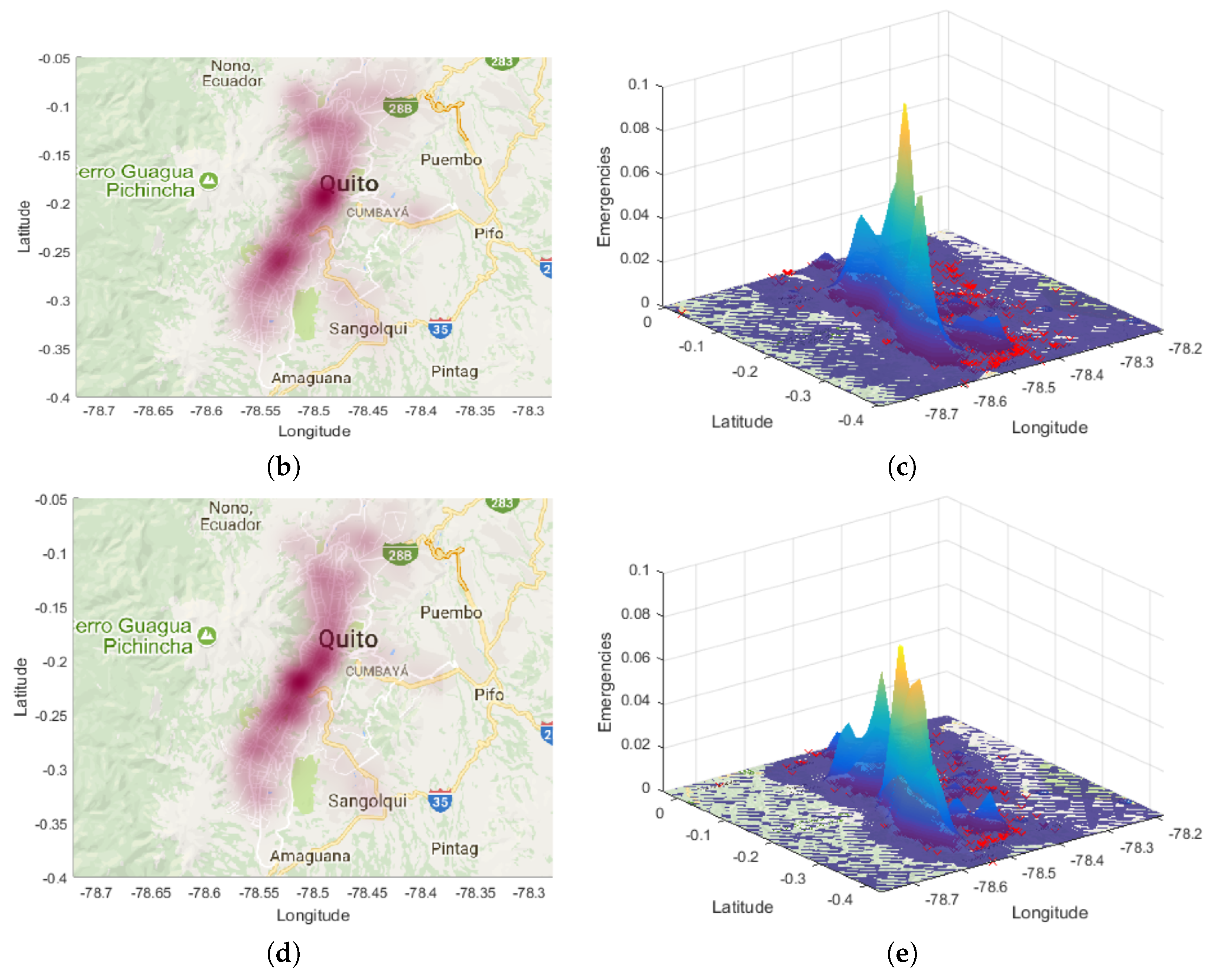
Figure 11.
Analysis of health emergencies. (a) Events during 2014, with maximum and minimum peaks; (b,c) Parzen distribution in red gradient over the map and bidimensional probability density function (PDF) representation for maximum peak on 1 January; (d,e) The same for minimum peak on 6 August.
Figure 11.
Analysis of health emergencies. (a) Events during 2014, with maximum and minimum peaks; (b,c) Parzen distribution in red gradient over the map and bidimensional probability density function (PDF) representation for maximum peak on 1 January; (d,e) The same for minimum peak on 6 August.

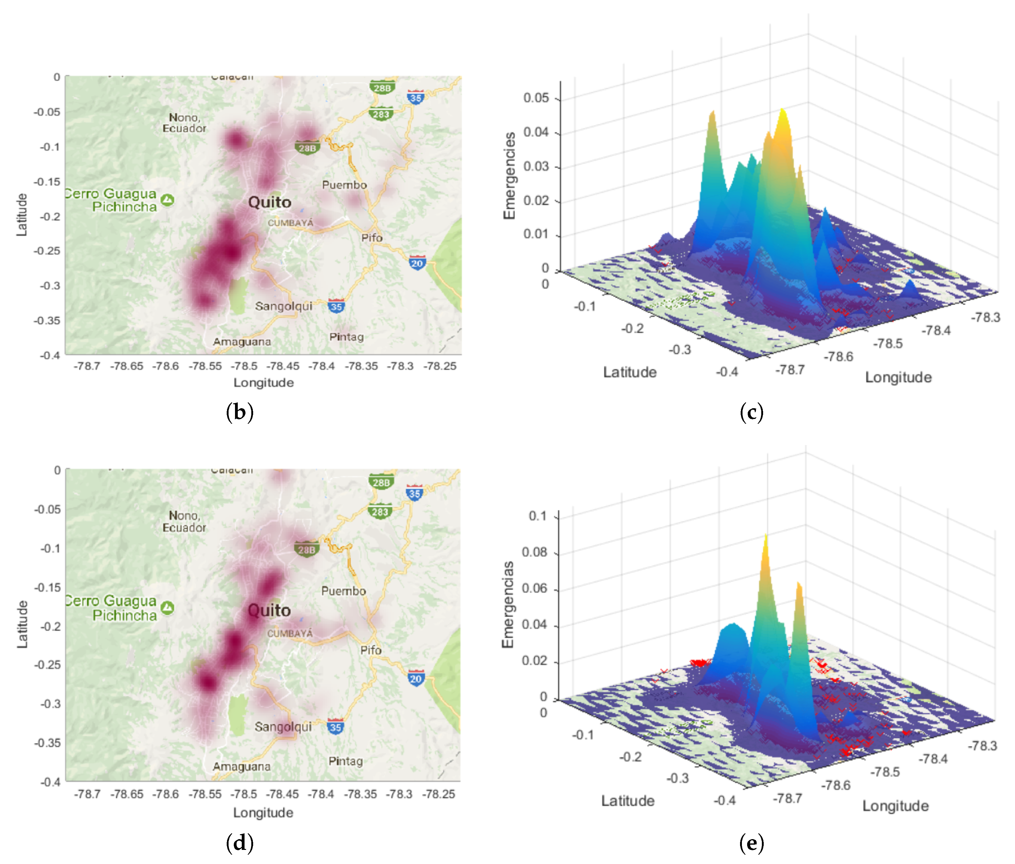
Figure 12.
Analysis of transit emergencies. (a) Events during 2014, with maximum and minimum peaks; Typical Parzen distribution (red gradient over the map) of transit emergencies registered on a weekend (b); and on weekdays (c) of a week in December.
Figure 12.
Analysis of transit emergencies. (a) Events during 2014, with maximum and minimum peaks; Typical Parzen distribution (red gradient over the map) of transit emergencies registered on a weekend (b); and on weekdays (c) of a week in December.


Figure 13.
Analysis of fire brigade emergencies. (a) Events during 2014, with maximum and minimum peaks; (b,c) Parzen distribution in red gradient over the map and bidimensional probability density function (PDF); (d,e) Parzen kernel density deviation via diffusion (KDD) representations for maximum peaks, circled in red, during 21 September. Parzen–KDD permits us to visualize in short scale the exact location of events on the sectors of Carretas (A) and Tumbaco (B), respectively.
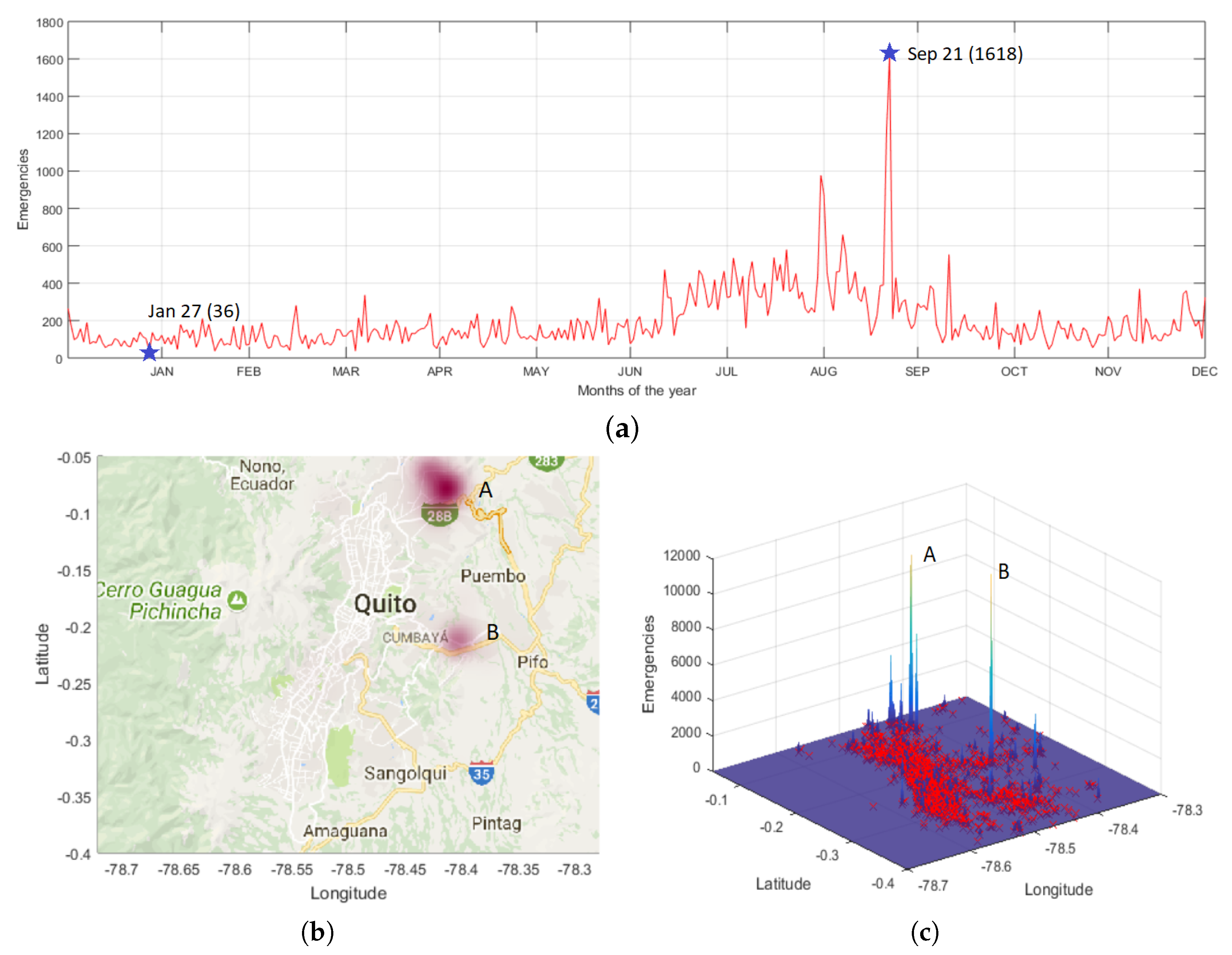
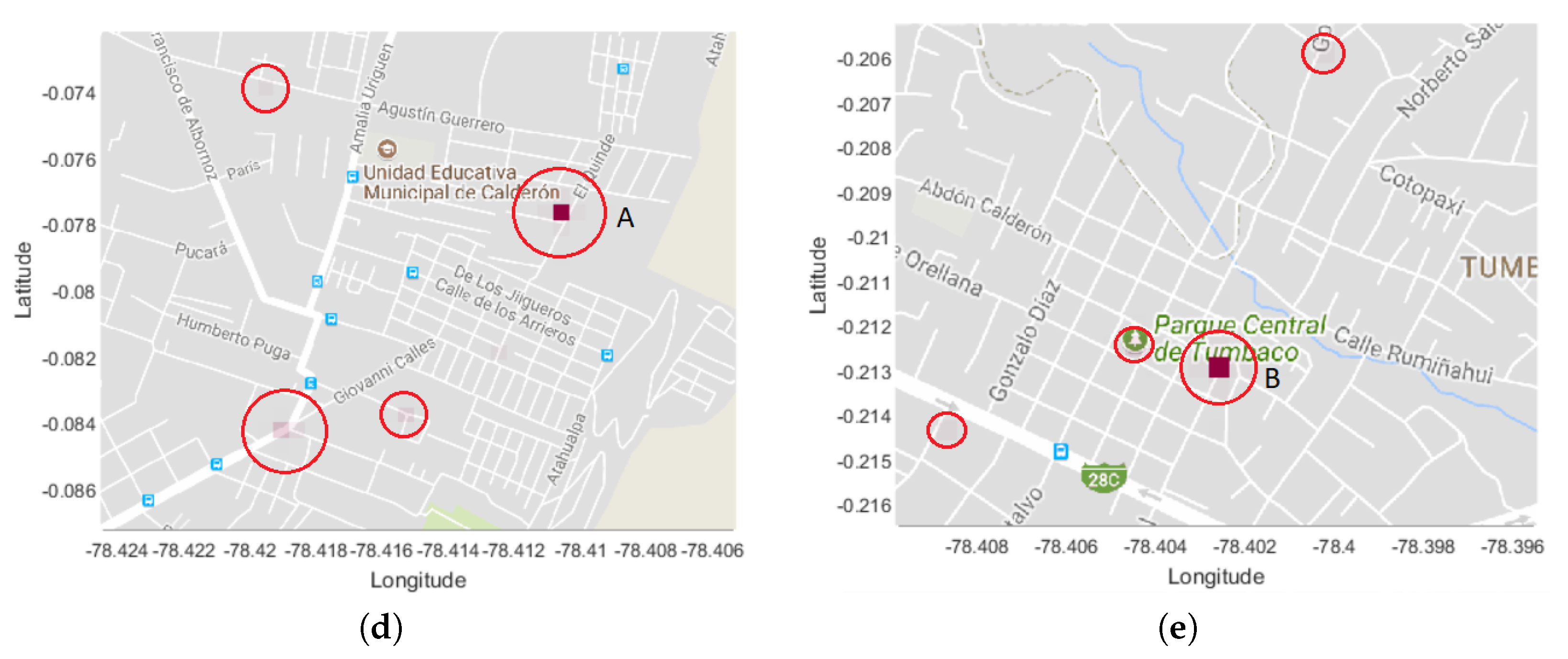
Figure 14.
Scatterplot of the emergencies registered during January 2014 in (a) the three main cities of the provinces covered by the public safety answering point (PSAP); (b) Tena, the capital of Napo; and (c) El Coca, the capital of Orellana.
Figure 14.
Scatterplot of the emergencies registered during January 2014 in (a) the three main cities of the provinces covered by the public safety answering point (PSAP); (b) Tena, the capital of Napo; and (c) El Coca, the capital of Orellana.


Table 1.
Percentage of emergencies attended during 2014 by the first response institutions (FRIs) of the public safety answering point (PSAP) in Quito, Ecuador.
Table 1.
Percentage of emergencies attended during 2014 by the first response institutions (FRIs) of the public safety answering point (PSAP) in Quito, Ecuador.
| Institution | Percentage |
|---|---|
| Police | 64.2 |
| Health services | 15.0 |
| Transit | 12.8 |
| Fire brigades | 3.0 |
| Municipal services | 2.8 |
| Military forces | 1.3 |
| Risk management secretaries | 0.9 |
© 2018 by the authors. Licensee MDPI, Basel, Switzerland. This article is an open access article distributed under the terms and conditions of the Creative Commons Attribution (CC BY) license (http://creativecommons.org/licenses/by/4.0/).
Share and Cite
MDPI and ACS Style
Corral-De-Witt, D.; Carrera, E.V.; Muñoz-Romero, S.; Rojo-Álvarez, J.L. Statistical, Spatial and Temporal Mapping of 911 Emergencies in Ecuador. Appl. Sci. 2018, 8, 199. https://doi.org/10.3390/app8020199
AMA Style
Corral-De-Witt D, Carrera EV, Muñoz-Romero S, Rojo-Álvarez JL. Statistical, Spatial and Temporal Mapping of 911 Emergencies in Ecuador. Applied Sciences. 2018; 8(2):199. https://doi.org/10.3390/app8020199
Chicago/Turabian StyleCorral-De-Witt, Danilo, Enrique V. Carrera, Sergio Muñoz-Romero, and José Luis Rojo-Álvarez. 2018. "Statistical, Spatial and Temporal Mapping of 911 Emergencies in Ecuador" Applied Sciences 8, no. 2: 199. https://doi.org/10.3390/app8020199
Note that from the first issue of 2016, this journal uses article numbers instead of page numbers. See further details here.