A Parallel Approach for Frequent Subgraph Mining in a Single Large Graph Using Spark

Abstract

Frequent subgraph mining (FSM) plays an important role in graph mining, attracting a great deal of attention in many areas, such as bioinformatics, web data mining and social networks. In this paper, we propose SSiGraM (Spark based Single Graph Mining), a Spark based parallel frequent subgraph mining algorithm in a single large graph. Aiming to approach the two computational challenges of FSM, we conduct the subgraph extension and support evaluation parallel across all the distributed cluster worker nodes. In addition, we also employ a heuristic search strategy and three novel optimizations: load balancing, pre-search pruning and top-down pruning in the support evaluation process, which significantly improve the performance. Extensive experiments with four different real-world datasets demonstrate that the proposed algorithm outperforms the existing GraMi (Graph Mining) algorithm by an order of magnitude for all datasets and can work with a lower support threshold.

1. Introduction

Many relationships among objects in a variety of applications such as chemical, bioinformatics, computer vision, social networks, text retrieval and web analysis can be represented in the form of graphs. Frequent subgraph mining (FSM) is a well-studied problem in the graph mining area which boosts many real-world application scenarios such as retail suggestion engines [1], protein–protein interaction networks [2], relationship prediction [3], intrusion detection [4], event prediction [5], text sentiment analysis [6], image classification [7], etc. For example, mining frequent subgraphs from a massive event interaction graph [8] can help to find recurring interaction patterns between people or organizations which may be of interest to social scientists.

There are two broad categories of frequent subgraph mining: (i) graph transaction-based FSM; and (ii) single graph-based FSM [9]. In graph transaction-based FSM, the input data comprise a collection of small-size or medium-size graphs called transactions, i.e., a graph database. In single graph-based FSM, the input data comprise one very large graph. The FSM task is to enumerate all subgraphs with support above the minimum support threshold. Graph transaction-based FSM uses transaction-based counting support while single graph-based FSM adopts occurrence-based counting. Mining frequent subgraphs in a single graph is more complicated and computationally demanding because multiple instances of identical subgraphs may overlap. In this paper, we focus on frequent subgraph mining in a single large graph.

The “bottleneck” for frequent subgraph mining algorithms on a single large graph is the computational complexity incurred by the two core operations: (i) efficient generation of all subgraphs with various size; and (ii) subgraph isomorphism evaluation (support evaluation), i.e., determining whether a graph is an exact match of another one. Let N and n be the number of vertexes of input graph G and subgraph S, respectively. Typically, the complexity of subgraph generation is $\mathcal{O}(2^{N^2})$ and support evaluation is $\mathcal{O}(N^n)$. Thus, the total complexity of an FSM algorithm is $\mathcal{O}(2^{N^2}·N^n)$, which is exponential in terms of problem size. In recent years, numerous algorithms for single graph-based FSM have been proposed. Nevertheless, most of them are sequential algorithms that require much time to mine large datasets, including SiGraM (Single Graph Mining) [10], GERM (Graph Evolution Rule Miner) [11] and GraMi (Graph Mining) [12]. Meanwhile, researchers have also used parallel and distributed computing techniques to accelerate the computation, in which two parallel computing frameworks are mainly used: Map-Reduce [13,14,15,16,17,18] and MPI (Message Passing Interface) [19]. The existing MapReduce implementations of parallel FSM algorithms are all based on Hadoop [20] and are designed for graph transaction and not for a single graph, often reaching IO (Input and Output) bottlenecks because they have to spend a lot of time moving the data/processes in and out of the disk during iteration of the algorithms. Besides, some of these algorithms cannot support mining via subgraph extension [14,15]. That is to say, users must provide the size of subgraph as input. In addition, although the MPI based methods, such as DistGraph [19], usually have a good performance, it is geared towards tightly interconnected HPC (High Performance Computing) machines, which are less available for most people. In addition, for MPI-based algorithms, it is hard to combine multiple machine learning or data mining algorithms into a single pipeline from distributed data storage to feature selection and training, which is common for machine learning. Fault tolerance is also left to the application developer.

In this paper, we propose a parallel frequent subgraph mining algorithm in a single large graph using Apache Spark framework, called SSiGraM. The Spark [21] is an in-memory MapReduce-like general-purpose distributed computation platform which provides a high-level interface for users to build applications. Unlike previous MapReduce frameworks such as Hadoop, Spark mainly stores intermediate data in memory, effectively reducing the number of disk input/output operations. In addition, a benefits of the “ML (Machine Learning) Pipelines” design [22] in Spark is that we can not only mine frequent subgraphs efficiently but also easily combine the mining process seamlessly with other machine learning algorithms like classification, clustering or recommendation.

Aiming at the two computational challenges of FSM, we conduct the subgraph extension and support evaluation across all the distributed cluster worker nodes. For subgraph extension, our approach generates all subgraphs in parallel through FFSM-Join (Fast Frequent Subgraph Mining) and FFSM-Extend proposed by Huan et al. [23], which is an efficient solution for candidate subgraphs enumeration. When computing subgraph support, we adopt the constraint satisfaction problem (CSP) model proposed in [12] as the support evaluation method. The CSP support satisfies the downward closure property (DCP), also known as anti-monotonic (or Apriori property), which means that a subgraph g is frequent if and only if all of its subgraphs are frequent. As a result, we employ a breadth first search (BFS) strategy in our SSiGraM algorithm. At each iteration, the generated subgraphs are distributed to every executor across the Spark cluster for solving the CSP. Then, the infrequent subgraphs are removed while the remaining frequent subgraphs are passed to the next iteration for candidate subgraph generation.

In practice, the support evaluation is more complicated than subgraph extension and will cost most time during the mining process. As a result, besides parallel mining, our SSiGraM algorithm also employs a heuristic search strategy and three novel optimizations: load balancing, pre-search pruning and top-down pruning in the support counting process, which significantly improve the performance. Noteworthily, SSiGraM can also be applied to directed graphs, weighted subgraph mining or uncertain graph mining with slight modifications introduced in [24,25]. In summary, our main contributions to the frequent subgraph mining in a single large graph are three-pronged:

• First, we propose SSiGraM, a novel parallel frequent subgraph mining algorithm in a single large graph using Spark, which is different from the Hadoop MapReduce based and MPI based parallel algorithms. SSiGraM can also easily combine with the bottom Hadoop distributed storage data and other machine learning algorithms.
• Second, we conduct in parallel subgraph extension and support counting, respectively, aiming at the two core steps with high computational complexity in frequent subgraph mining. In addition, we provide a heuristic search strategy and three optimizations for the support computing operation.
• Third, extensive experimental performance evaluations are conducted with four real-world graphs. The proposed SSiGraM algorithm outperforms the GraMi method by at least one order of magnitude with the same memory allocated.

The paper is organized as follows. The problem formalization is provided in Section 2. Our SSiGraM algorithm and its optimizations are presented in Section 3. In Section 4, extensive experiments to evaluate the performance of the proposed algorithm are conducted and analyzed. The work is summarized and conclusions are drawn in Section 5.

2. Formalism

A graph $G=(V,E)$ is defined to be a set of vertexes (nodes) V which are interconnected by a set of edges (links) $E\subseteq V\times V$ [26]. A labelled graph also consists of a labeling function L besides V and E that assigns labels to V and E. Usually, the graphs used in FSM are assumed to be labelled simple graphs, i.e., un-weighted and un-directed labeled graphs with no loops and no multiple links between any two distinct nodes [27]. To simplify the presentation, our SSiGraM is illustrated with an undirected graph with a single label for each node and edge. Nevertheless, as mentioned above, the SSiGraM can also be extended to support either directed or weighted graphs. In the following, a number of widely used definitions used later in this paper are introduced.

Definition 1.

(Labelled Graph): A labelled graph can be represented as $G=(V,E,L_V,L_E,\phi )$, where V is a set of vertexes, $E\subseteq V\times V$ a set of edges. $L_V$ and $L_E$ are sets of vertex and edge labels respectively. ϕ is a label function that defines the mappings $V\to L_V$ and $E\to L_E$.

Definition 2.

(Subgraph): Given two graphs $G_1=(V_1,E_1,L_{V_1},L_{E_1},{\phi }_1)$ and $G_2=(V_2,E_2,L_{V_2},L_{E_2},{\phi }_2)$, $G_1$ is a subgraph of $G_2$, if and only if (i) $V_1\subseteq V_2$, and $\forall v\in V_1$, ${\phi }_1\left(v\right)={\phi }_2\left(v\right)$; (ii) $E_1\subseteq E_2$, and $\forall (u,v)\in E_1$, ${\phi }_1(u,v)={\phi }_2(u,v)$. $G_2$ is also called a supergraph of $G_1$.

Definition 3.

(Subgraph Isomorphism): Let $G_1=(V_1,E_1,L_{V_1},L_{E_1},{\phi }_1)$ be a subgraph of G. $G_1$ is subgraph isomorphic to graph G, if and only if there exists another subgraph $G_2=(V_2,E_2,L_{V_2},L_{E_2},{\phi }_2)\subseteq G$ and a bijection $f:V_1\to V_2$ satisfying: (i) $\forall u\in V_1$, ${\phi }_1\left(u\right)={\phi }_2\left(f\left(u\right)\right)$; (ii) $\forall (u,v)\in E_1\iff (f\left(u\right),f\left(v\right))\in E_2$; and (iii) $\forall (u,v)\in E_1$, ${\phi }_1(u,v)={\phi }_2(f\left(u\right),f\left(v\right))$. $G_2$ is also called an embedding of $G_1$ in G.

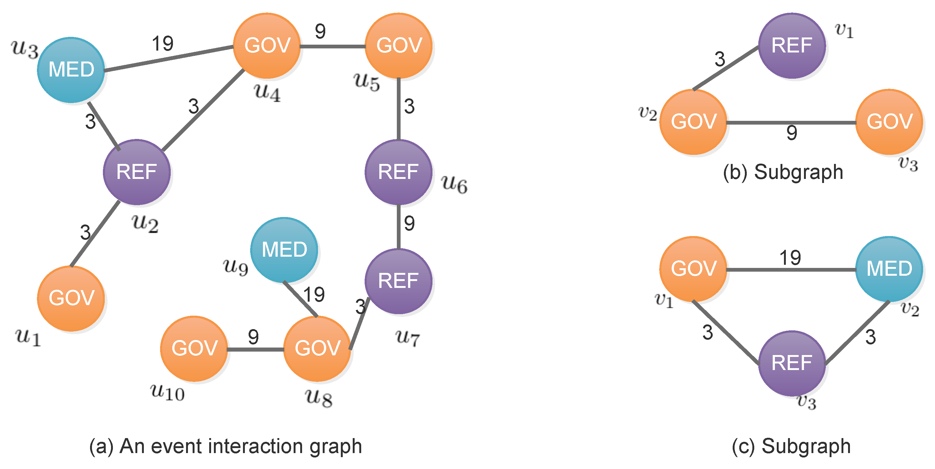
For example, Figure 1a illustrates a labelled graph of event interaction graph. Node labels represent the event actor’s type (e.g., GOV: government) in CAMEO (Conflict And Mediation Event Observations) codes [28] and edge labels represent the event type [28] between the two actors. Figure 1b,c shows two subgraphs of Figure 1a. Figure 1b ($v_1\stackrel{3}{-}{v}_2\stackrel{9}{-}{v}_3$) has three isomorphisms with respect to graph (a): $u_2\stackrel{3}{-}{u}_4\stackrel{9}{-}{u}_5$, $u_6\stackrel{3}{-}{u}_5\stackrel{9}{-}{u}_4$ and $u_7\stackrel{3}{-}{u}_8\stackrel{9}{-}{u}_{10}$.

Definition 4.

(Frequent Subgraph in Single Graph): Given a labelled single graph G and a minimum support threshold τ, the frequent subgraph mining problem is defined as finding all subgraphs $G_i$ in G,

$$Sup(G_i,G)\ge \tau ,\forall G_i\in S,$$

where S denotes the set of subgraphs in G with support greater or equal to τ.

For a subgraph $G_1$ and input graph G, the straightforward way to compute the support of $G_1$ in graph G is to count all its isomorphisms of $G_1$ in G [29]. Unfortunately, such a method does not satisfy the downward closure property (DCP) since there are cases where a subgraph appears fewer times than its supergraph. For example, in Figure 1a, the single node graph REF (Refugee) appears three times, while its supergraph REF$\stackrel{3}{-}$GOV appears four times. Without the DCP, the search space cannot be pruned and the exhaustive search is unavoidable [30]. To address this issue, we employ the minimum image (MNI) based support which is anti-monotonic introduced in [31].

Definition 5.

(MNI Support): For a subgraph $G_1$, let $\sum \left(S\right)=\{{\varphi }_1,{\varphi }_2,\dots ,{\varphi }_m\}$ denote the set of all isomorphisms/embeddings of $G_1$ in the input graph G. The MNI support of a subgraph $G_1$ in G is based on the number of unique nodes in the input graph G that a node of the subgraph $G_1=(V_1,E_1)$ is mapped to, which is defined as:

$$Su{p}_{MNI}(G_1,G)=\underset{v\in V_1}{min}\left\{\right|\Phi \left(v\right)\left|\right\},$$

where $\Phi \left(v\right)$ is the set of unique mappings for each $v\in V_1$, denoted as

$$\Phi \left(v\right)=\bigcup _{i=1}^{|\sum (S\left)\right|}{\varphi }_i\left(v\right).$$

Figure 2 illustrates the four isomorphisms of a subgraph $G_1\equiv A$-B-C-A in the input graph. For example, one of the isomorphisms is $\varphi =\{u_1,u_4,u_6,u_8\}$, shown in the second column in Figure 2c. There are four isomorphisms for the subgraph $G_1$ in Figure 2b. Therefore, the set of unique mappings for the vertex $v_1$ is $\{u_1,u_2,u_8\}$. The number of unique mappings over all the subgraph vertices $\{v_1,v_2,v_3,v_4\}$ are 3, 3, 2 and 2, respectively. Thus, the MNI support of $G_1$ is $Su{p}_{MNI}(G_1,G)=min\{3,3,2,2\}$ = 2.

Definition 6.

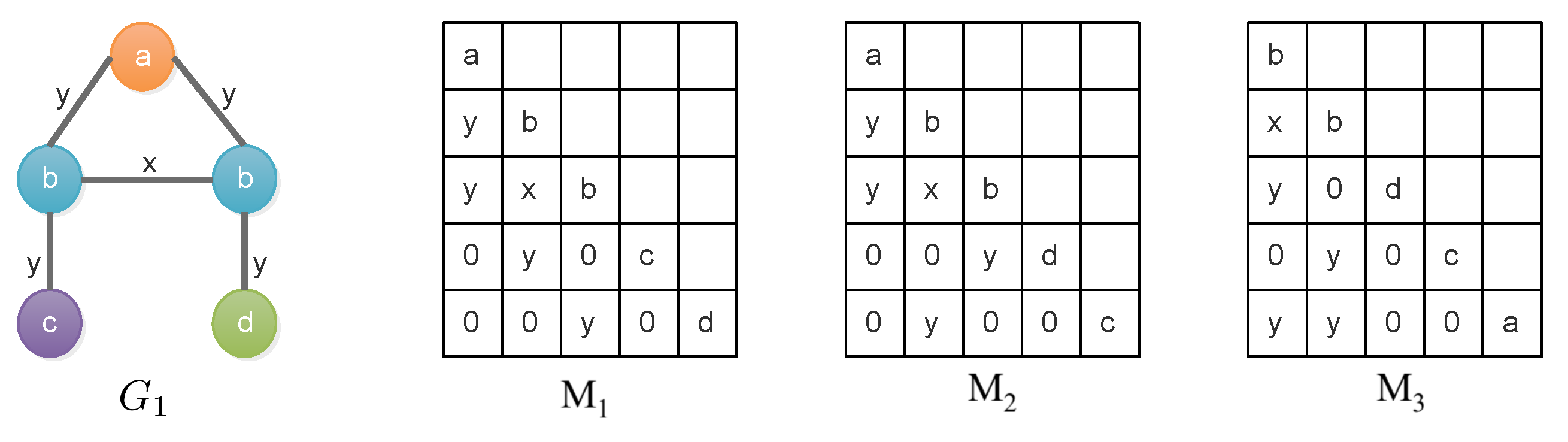
(Adjacency Matrix): The adjacency matrix of a graph $G_i$ with n vertexes is defined as a $n\times n$ matrix M, in which every diagonal entry corresponds to a distinct vertex in $G_i$ and is filled with the label of this vertex and every off-diagonal (for an undirected graph, the upper triangle is always a mirror of the lower triangle) entry in the lower triangle part corresponds to a pair of vertices in $G_i$ and is filled with the label of the edge between the two vertices and zero if there is no edge.

Definition 7.

(Maximal Proper Submatrix): For a $m\times m$ matrix A, a $n\times n$ matrix B is the maximal proper submatrix of A, iff B is obtained by removing the last nonzero entry from A. For example, the last non-zero entry of $M_2$ in Figure 3 is y in the bottom row.

Definition 8.

(Canonical Adjacency Matrix): Let matrix M denote the adjacency matrix of graph $G_i$. $Code\left(M\right)$ represents the code of M, which is defined as the sequence formed by concatenating lower triangular entries of M (including entries on the diagonal) from left to right and top to bottom, respectively. The canonical adjacency matrix (CAM) of graph $G_i$ is the one that produces the maximal code, using lexicographic order [23]. Obviously, a CAM’s maximal proper submatrix is also a CAM.

Figure 3 shows three adjacency matrices $M_1$, $M_2$, $M_3$ for the graph $G_1$ on the left. After applying the standard lexicographic order, we have $Code\left(M_1\right):aybyxb0y0c00y0d>Code\left(M_2\right):aybyxb00yd0y00c>Code\left(M_3\right):bxby0d0y0cyy00a$. In fact, $M_1$ is the canonical adjacency matrix of $G_1$.

Definition 9.

(Suboptimal CAM): Given a graph G, a suboptimal canonical adjacency matrix (suboptimal CAM) of G is an adjacency matrix M of G such that its maximal proper submatrix N is the CAM of the graph that N represents. [23]. A CAM is also a suboptimal CAM. A proper suboptimal CAM is denoted as a suboptimal CAM that is not the CAM of the graph it represents.

3. The SSiGraM Approach

This section first elaborates upon the framework of the proposed algorithm, before describing the detailed procedure of parallel subgraph extension, parallel support evaluation and three optimization strategies.

3.1. Framework

Figure 4 illustrates the proposed framework of our SSiGraM approach. It mainly contains two major components: parallel subgraph extension and parallel support evaluation. The green notations are main Spark RDD (a resilient distributed dataset (RDD) is the core abstraction of Spark, which is a fault-tolerant collection of elements that can be operated on in parallel) transformations or actions used during the algorithm pipeline, e.g., map, join, etc. We will discuss details of the framework below.

3.2. Parallel Subgraph Extension

Our approach employs a breadth first search (BFS) strategy that generates all subgraphs in parallel through FFSM-Join and FFSM-Extend proposed in [23]. Similarly, we organize all the suboptimal CAMs of subgraphs in a graph G into a rooted tree, that follows the rules: (i) The root of the tree is an empty matrix. (ii) Each node in the tree is a distinct subgraph of G, represented by its suboptimal CAM that is either a CAM or a proper suboptimal CAM. (iii) For a given non-root node (with suboptimal CAM M), its parent is the graph represented by the maximal proper submatrix of M. The completeness of the suboptimal CAM tree is guaranteed by the Theorem 1. For the formal proof, we refer to the appendix in [23].

Theorem 1.

For a graph G, let $C_{k-1}$ and $C_k$ be sets of the suboptimal CAMs of all the subgraphs with $(k-1)$ edges and k edges ($k\ge 2$). Every member of set $C_k$ can be enumerated unambiguously either by joining two members of set $C_{k-1}$ or by extending a member in $C_{k-1}$.

Algorithm 1 shows how the subgraph extension process is conducted in parallel. Actually, the extension process is implemented in parallel at the parent subgraph scale (Lines 6–15), which means that each group of subgraphs with the same parent will be sent to an executor for extension in the Spark cluster. The FFSM operator is provided by [32], which implements the FFSM-Join and FFSM-Extend. After extension, all of the extended results are collected to the driver node (Line 16) from the cluster. Because of the extension on more than one executors at the same time, the indexes of the new generated subgraphs from different executors may be duplicated. As a result, the subgraph indexes are reassigned at the end (Line 17).

To perform a parallel subgraph extension, Line 11 and Line 13 conduct the joining and extension of CAM across all Spark executors. The overall complexity is $\mathcal{O}(n^2·m)$ where n is the number of nodes in subgraph and m number of edges. A complete graph with n vertices consists of $n(n-1)/2$ edges. Thus, the final complexity is $\mathcal{O}\left(m^2\right)$.

Algorithm 1 Parallel Subgraph Extension.

Input: frequent subgraphs $S_{k-1}$, broadcasted FFSM operator $FFSMRDD$, Spark context $sc$ Output: new generated $S_k$ that extend $S_{k-1}$ 1: function ParaGenSubgraphs($S_{k-1}$,$FFSMRDD$,$sc$) 2:      $S_k\leftarrow ⌀$ 3:      $FFSMOperator\leftarrow FFSMRDD$ 4:      $PGrap{h}_{S_{k-1}}\leftarrow S_{k-1}$, group by parents 5:      $PGraphRD{D}_{S_{k-1}}\leftarrow sc.\mathbf{parallelize}\left(PGrap{h}_{S_{k-1}}\right)$ 6:      $S_k\leftarrow PGraphRD{D}_{S_{k-1}}.\mathbf{map}\{$ 7:      $S_t\leftarrow ⌀$ 8:      $C_{list}\leftarrow$ child subgraphs of present parent 9:      for $s_i$ in $C_{list}$ do 10:          for $s_j$ in $C_{list}$ do 11:               $S_t\leftarrow S_t\cup FFSMOperator.join(s_i,s_j)$ 12:          end for 13:          $S_t\leftarrow S_t\cup FFSMOperator.extend\left(s_i\right)$ 14:      end for 15:      return $S_t$ 16:      }.collect 17:      reassign subgraph indexes in $S_k$ 18:      return $S_k$ 19: end function

3.3. Parallel Support Evaluation

Our SSiGraM approach employs the CSP model [12] as the subgraph support evaluation strategy. The constraint satisfaction problem (CSP) is an efficient method for finding subgraph isomorphisms (Definition 3), which is illustrated as follows:

Definition 10.

(CSP Model): Let $G_1=(V_1,E_1,L_{V_1},L_{E_1},{\phi }_1)$ be a subgraph of a graph $G=(V,E,L_V,L_E,\phi )$. Finding isomorphisms of $G_1$ in G is a CSP($\mathcal{X},\mathcal{D},\mathcal{C}$) where:

1. 

$\mathcal{X}$ is an ordered set of variables which contains a variable $x_v$ for each node $v\in V_1$.

2. 

$\mathcal{D}$ is the set of domains for each variable $x_v\in \mathcal{X}$ . Each domain is a subset of V.

3. 

Set $\mathcal{C}$ contains the following constraint rules:

• $\forall x_v,x_{v^{\prime }}\in \mathcal{X}$, $x_v\ne x_{v^{\prime }}$.
• $\forall x_v\in \mathcal{X}$ and the corresponding $v\in V_1$, $\phi \left(x_v\right)={\phi }_1\left(v\right)$.
• $\forall x_v,x_{v^{\prime }}\in \mathcal{X}$ and the corresponding $v,v^{\prime }\in V_1$, $\phi (x_v,x_{v^{\prime }})={\phi }_1(v,v^{\prime })$.

For example, the CSP model of a subgraph in Figure 1b under graph Figure 1a is:

$$\left(\begin{array}{c}\mathcal{X}:\{x_{v_1},x_{v_2},x_{v_3}\},\\ \mathcal{D}:\{\{u_1,u_2,\dots ,u_{10}\},\{u_1,u_2,\dots ,u_{10}\},\{u_1,u_2,\dots ,u_{10}\}\},\\ \mathcal{C}:\{x_{v_1}\ne x_{v_2}\ne x_{v_3},\\ \phi \left(v_1\right)=\mathrm{REF},\phi \left(v_2\right)=\mathrm{GOV},\phi \left(v_3\right)=\mathrm{GOV},\\ \phi (v_1,v_2)=3,\phi (v_2,v_3)=9\}\end{array}\right)$$

Theorem 2 [12] describes the relation between subgraph isomorphism and the CSP model. Intuitively, the CSP model is similar to a template, in which each variable in $\mathcal{X}$ is a slot. A solution is a correct slot fitting which assigns a different node of G to each node of $G_1$, such that the labels of the corresponding nodes and edges match. For instance, a solution to the CSP of the above example is the assignment $(x_{v_1},x_{v_2},x_{v_3})=(u_2,u_4,u_5)$. If there exists a solution that assigns a node u to variable $x_v$, then this assignment is valid. $x_{v_1}=u_2$ is a valid assignment while $x_{v_1}=u_1$ is invalid in this example.

Theorem 2.

A solution of the subgraph $G_1$ to graph G CSP corresponds to a subgraph isomorphism of $G_1$ to G.

Theorem 3.

Let ($\mathcal{X},\mathcal{D},\mathcal{C}$) be the subgraph CSP of $G_1$ under graph G. The MNI support of $G_1$ in G satisfying:

$$Su{p}_{MNI}(G_1,G)\ge \tau \iff \forall x_v\in \mathcal{X},AS{S}_{valid}\left(x_v\right)\ge \tau .$$

where $AS{S}_{valid}\left(x_v\right)$ is the total count of valid assignments of variable $x_v$.

According to Theorem 3 [12], we can consider the CSP of subgraph $G_1$ to graph G and check the count of valid assignments of each variable. If there exist $\tau$ or more valid assignments for every variable, in other words, at least $\tau$ nodes in each domain $D_1,\dots ,D_n$ for the corresponding variables $x_{v_1},\dots ,x_{v_n}$, then subgraph $G_1$ is frequent under the MNI support. Thus, the main idea of the heuristic search strategy is elaborated as: if any variable domain remains with less than $\tau$ candidates during the search process, then the subgraph cannot be frequent.

3.4. Optimizing Support Evaluation

After subgraph extension, all the new generated subgraphs are sent to the next procedure for support evaluation. As mentioned in the Introduction, support evaluation is an NP-hard problem which takes $\mathcal{O}\left(N^n\right)$ time. The complexity is exponential if we brutally search all the valid assignments.

Owing to the iterative and incremental design of RDD and the join transformation in Spark, we save the CSP domain data of every generated subgraph. As the two green labels join shown in Figure 4, the first join operation combines the new generated subgraphs and frequent edges to get the extended edges, while the second join combines new generated subgraphs and extended edges to generate the search space, i.e., the CSP domain data. In addition, to speed up the support evaluation process, we also propose three optimizations, namely, load balancing, pre-search pruning and top-down pruning, the execution order of which is illustrated on the headpiece of Figure 4.

3.4.1. Load Balancing

The support evaluation process is implemented in parallel at subgraph scale, which means that each subgraph will be sent to an executor in the Spark cluster for support evaluation. The search space is highly dependent on the subgraph’s CSP domain size. Nevertheless, new subgraphs may have different domain sizes which result in the phenomenon that some executors may finish searching fast while others are very slow. The final execution time of the whole cluster depends upon the last finished executor.

To overcome this unbalance, generally, the subgraphs distributed to various executors must have roughly the same domain sizes. Algorithm 2 illustrates the detailed process. Because the domain of the present subgraph is incrementally generated from the parent subgraph’s domain of last iteration, we save the domain sizes of all subgraphs in each iteration. Then, according to the saved domain sizes of parent subgraphs, new generated subgraphs are re-ordered and partitioned to different executors (Lines 6–9).

Let n be the number of nodes of subgraph S, i.e., the domain size. Load balancing can be done in $\mathcal{O}\left(n\right)$ time.

Algorithm 2 Load Balancing

Input: RDD of subgraph set $SRDD$, Spark cluster parallelism n, Spark context $sc$ Output: $SRD{D}_{balance}$: balanced RDD of subgraph set 1: function LoadBalancing($SRDD$,n,$sc$) 2:      $S_{balance}\leftarrow ⌀$ 3:      $S\leftarrow SRDD$ 4:      sort S in descending domain size order 5:      initialize n empty partitions 6:      for s in S do 7:           $S_{balance}\left(p\right)\leftarrow$smallest partition 8:           add s to partition $S_{balance}\left(p\right)$ 9:      end for 10:      $SRD{D}_{rp}\leftarrow sc.parallelize(S_{balance},n)$ 11:      return $SRD{D}_{balance}$ 12: end function

3.4.2. Pre-Search Pruning

Because the input single large graph we consider is an undirected labeled graph, if a node and its neighbors have the same node label and edges between them also have the same label, it will bring redundant search space. This phenomenon can be common in graphs, especially when the graphs have few node labels and edge labels. For example, in Figure 5, G is the input graph and $G_1$ a subgraph. The CSP search space of $G_1$ is illustrated at the bottom. The assignments in dashed lines are added to the search space when iteratively building the CSP domain data of $G_1$ whereas they are redundant space violating the first rule in Definition 10. Here, $u_1$ is assigned twice to $v_1$ and $v_3$ ({$u_1,u_2,u_1$}, {$u_1,u_3,u_1$}, {$u_1,u_4,u_1$}). If this redundant search space is pruned before calculating the actual support, the search speed will be much accelerated.

Let N and n be the number of nodes of input graph G and subgraph S. Pre-search pruning will search for redundant space for every node of S between its neighbors in G, the complexity of which is $\mathcal{O}(n·N^3)$.

3.4.3. Top-Down Pruning

Either FFSM-Join operation or FFSM-Extend operation add an edge to the parent subgraph at a time when generating new subgraphs and constructing the suboptimal CAM tree. Therefore, as the parent subgraph at upside of suboptimal CAM tree is a substructure of its child subgraph, those assignments that were pruned from the domains of the parent, can also not be valid assignments for any of its children [12]. For instance, Figure 6a shows a part of a subgraph generation tree, which is constructed from $G_1$ which is extended to $G_2$ and $G_3$ and last, $G_4$ via $G_3$. The marked nodes in different colors represent the pruned assignments from the top to bottom. Invalid assignments from parent subgraphs are pruned from all their child subgraphs. Thus, the search space is reduced a lot. Take subgraph $G_4$ in Figure 6 as an example, when considering variable $x_{v_1}$, the search space has a size of $3\times 2\times 3\times 2=36$ combinations, while without top-down pruning the respective search space size is $5\times 3\times 5\times 4=300$ combinations.

Top-down pruning iterates for every node in S and for every value in each domain. Thus, the overall complexity is $\mathcal{O}(m·N)$.

After introducing pre-search pruning and top-down pruning, we give the pseudocode IsFrequent of heuristically checking whether a subgraph s is frequent in Algorithm 3. Pre-search pruning is conducted at Line 4 to Line 7 while top-down pruning Line 11 to Line 23.

3.5. The SSiGraM Algorithm

Finally, we show the detail pipeline of the SSiGraM approach in Algorithm 4. SSiGraM starts by loading the input graph using Spark GraphX (Line 2). Then all frequent edges are identified at Line 4. For each iteration, parallel subgraph extension is conducted at Line 11 and parallel support evaluation Line 14 to Line 22 in which load balancing, pre-search pruning and top-down pruning are conducted. The complexity of SSiGraM is $\mathcal{O}(n·N·(N^2+n)+n^4+n)$ based on the above processes.

Algorithm 3 Support Evaluation.

Input: A subgraph s, domain data $D_s$, threshold $\tau$ Output: true if s is a frequent subgraph of G, false otherwise 1: function IsFrequent($s,D_s,\tau$) 2:       for variable v in $D_s$ do 3:           get neighbors of v: $N\left(v\right)\leftarrow v$ 4:           if $N\left(v\right).size>1$ then 5:           for element u of $D_s\left(v\right)$ do 6:               remove redundant u 7:           end for 8:       end for 9:       if the size of any domain in $D_s$ is less than $\tau$ then 10:       return $false$ 11:       for variable v in $D_s$ do 12:           $count\leftarrow 0$ 13:           for element u of $D_s\left(v\right)$ do 14:               if u is already marked then 15:               $count$++ 16:               else if a solution that assigns u to v exists then 17:               Mark corresponding values in $D_s$ 18:               $count$++ 19:               else Remove u from v’s domain in $D_s$ 20:               if $count=\tau$ then 21:               Move to next variable v 22:             end for 23:       end for 24:       return $true$ 25: end function

4. Experimental Evaluation

In this section, the performance of the proposed algorithm SSiGraM is evaluated using four real-world datasets with different sizes from different domains. Firstly, the experimental setup is introduced. The performance of SSiGraM is then evaluated.

4.1. Experimental Setup

Dataset: We experiment on four real graph datasets, whose main characteristics are summarized in

Table 1. Datasets and their characteristics.

Dataset	#Node	#L(Node)	#Edge	#L(Edge)	Density
DBLP	151,574	7	191,840	17	Medium
Aviation	101,185	6173	133,087	41	Sparse
GDELT	1,515,712	14,816	2,832,692	8	Sparse
Twitter	11,316,811	40	85,331,846	1	Dense

.

Algorithm 4 The SSiGraM Algorithm.

Input: A graph G, support threshold $\tau$ and Spark context $sc$, parallelism n Output: All subgraphs S of G such that $Su{p}_{MNI}(S,G)\ge \tau$ 1: result $S\leftarrow ⌀$, intermediate subgrah set $S_{rdd}\leftarrow ⌀$ 2: load $Grap{h}_{rdd}$ from G using $sc.GraphX$ 3: detect connected areas of $Grap{h}_{rdd}$ 4: $FreEdg{e}_{rdd}\leftarrow Grap{h}_{rdd}$ 5: $FFSM\leftarrow FreEdg{e}_{rdd}$ 6: $FFS{M}_{rdd}=sc.\mathbf{broadcast}\left(FFSM\right)$ 7: initial frequent subgraphs $S_1\leftarrow FreEdg{e}_{rdd}$ 8: $S_{rdd}\leftarrow S_1$ 9: while $S_{rdd}.count>0$ do 10:     $S_{k-1}\leftarrow S_{rdd}$ 11:     $S_k\leftarrow$ParaGenSubgraphs($S_{k-1},FFS{M}_{rdd},sc$) 12:     $NewSu{b}_{rdd}\leftarrow S_k$ 13:     $OldSu{b}_{rdd}\leftarrow NewSu{b}_{rdd}.clone$ 14:     $ExtEdg{e}_{rdd}\leftarrow NewSu{b}_{rdd}$.join($FreEdg{e}_{rdd}$) 15:     $OldSu{b}_{rdd}\leftarrow$LoadBalancing($OldSu{b}_{rdd},n,sc$) 16:     $CandSu{b}_{rdd}\leftarrow OldSu{b}_{rdd}.$join($ExtEdg{e}_{rdd}$) 17:     $S_{rdd}\leftarrow CandSu{b}_{rdd}.$flatmap{ 18:         let current subgraph be s 19:         $D_s\leftarrow s$ 20:         if IsFrequent($s,D_s,\tau$) then 21:         return s 22:     }.collect 23:     $S\leftarrow S\cup S_{rdd}$ 24: end while 25: return S

DBLP (http://dblp.uni-trier.de/db/). The DBLP (DataBase systems and Logic Programming) bibliographic dataset models the co-authorship information and consists of 150 K nodes and nearly 200 K edges. Vertices represent authors and are labeled with the author’s field of interest. Edges represent collaboration between two authors and are labeled with the number of co-authored papers.

Aviation (http://ailab.wsu.edu/subdue/). This dataset contains a list of event records extracted from the aviation safety database. The events are transformed to a graph which consists of 100 K nodes and 133 K edges. The nodes represent event ids and attribute values. Edges represent attribute names and the “near_to” relationship between two events.

GDELT (https://bigquery.cloud.google.com/table/gdelt-bq:full.events?pli=1). This dataset is constructed from part of the raw events exported from the GDELT (Global Data on Events, Location and Tone) dataset. It consists of 1.5 M nodes and 2.8 M edges. Similar to the Aviation dataset, nodes represent events and attribute values (and are labeled with event types and actual attribute values). Edges represents attribute name and the “relate_to” relationship between two events.

Twitter (http://socialcomputing.asu.edu/datasets/Twitter). This graph models the social news of Twitter and consists of 11M nodes and 85 M edges. Each node represents a Twitter user and each edge represents an interaction between two users. The original graph does not have labels, so we randomly added 40 labels to the nodes, the randomization of which follows a Gaussian distribution. In detail, the mean value was set to 50 and the std-deviance 15. The generated vertex labels less than 0 were all set to 1.

Comparison Method: We compare the proposed SSiGraM algorithm with the GraMi [12] and we use the $GRAMI\_UNDIRECTED\_SUBGRAPHS$ version of GraMi provided by the authors.

Running Environment: All the experiments with SSiGraM are conducted on Apache Spark (version 1.6.1) deployed on Apache Hadoop YARN (version 2.7.1). The total executors is set to 20 with 6 GB memory and 1 core running at 2.4 GHz for each executor. The memory of driver program is also 6 GB and max results 2 GB. Thus, the total memory allocated from YARN is 128 GB. For the sake of fairness, GraMi is conducted on a Linux (Ubuntu 14.04) machine running at 2.4 GHz with 128 GB RAM.

Performance Metrics: The support threshold $\tau$ is the key evaluation metric as it determines whether a subgraph is frequent. Decreasing $\tau$ results in an exponential increase in the number of possible candidates and thus exponential decrease in the performance of the mining algorithms. For a given time budget, an efficient algorithm should be able to solve mining problems for low $\tau$ values. When $\tau$ is given, efficiency is determined by the running time. In addition, we also give the total subgraphs each algorithm identified under each $\tau$ value, proving the correctness of the SSiGraM algorithm.

4.2. Experimental Results

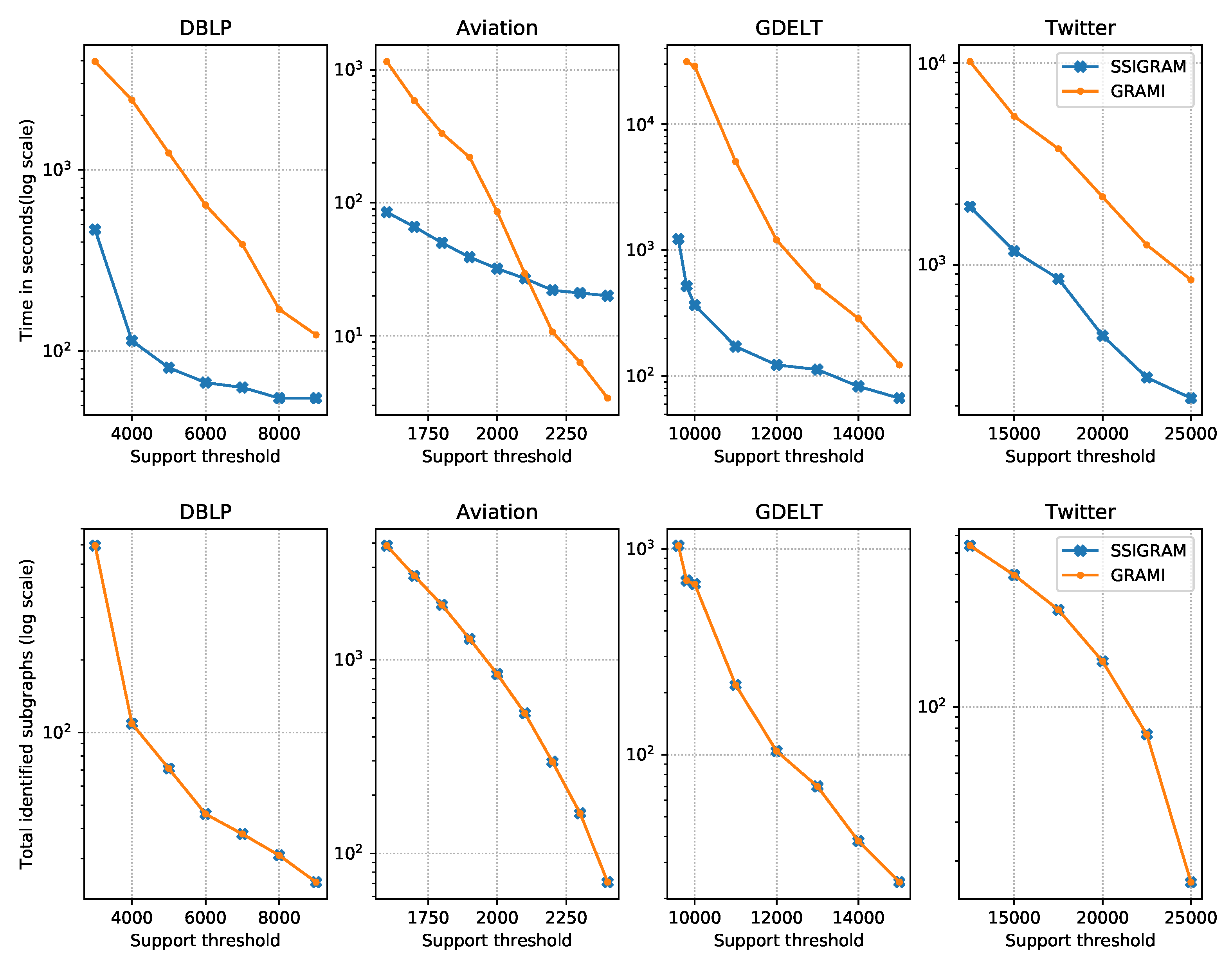
Performance: At the top part of Figure 7, we show the performance comparison between SSiGraM and GraMi on DBLP, Aviation, GDELT and Twitter datasets. The number of results grows exponentially when the support threshold $\tau$ decreases. Thus, the running time of all algorithms also grows exponentially. Our results indicate that SSiGraM outperforms GraMi by an order of magnitude for all datasets. For bigger dataset GDELT and lower $\tau$ (9600), GraMi ran out of memory and was not able to produce a result. For smaller dataset Aviation and bigger $\tau$ (2200, 2300 and 2400), GraMi is faster because the resource scheduling of Hadoop YARN in SSiGraM will cost 10 to 20 s. Actually, in this circumstance, there is no need to use parallel mining algorithms since GraMi can give results within a few seconds. For the Twitter dataset, SSiGraM is about five times faster than GraMi because of the existence of nodes with a big degree. When a subgraph involves such a node, SSiGraM will not go to the next iteration until the executor finishes calculating the support of this subgraph.

The bottom part of Figure 7 illustrates the total numbers of identified frequent subgraphs on each dataset. The identical numbers of frequent subgraphs of SSiGraM and GraMi elaborate the correctness of our SSiGraM algorithm.

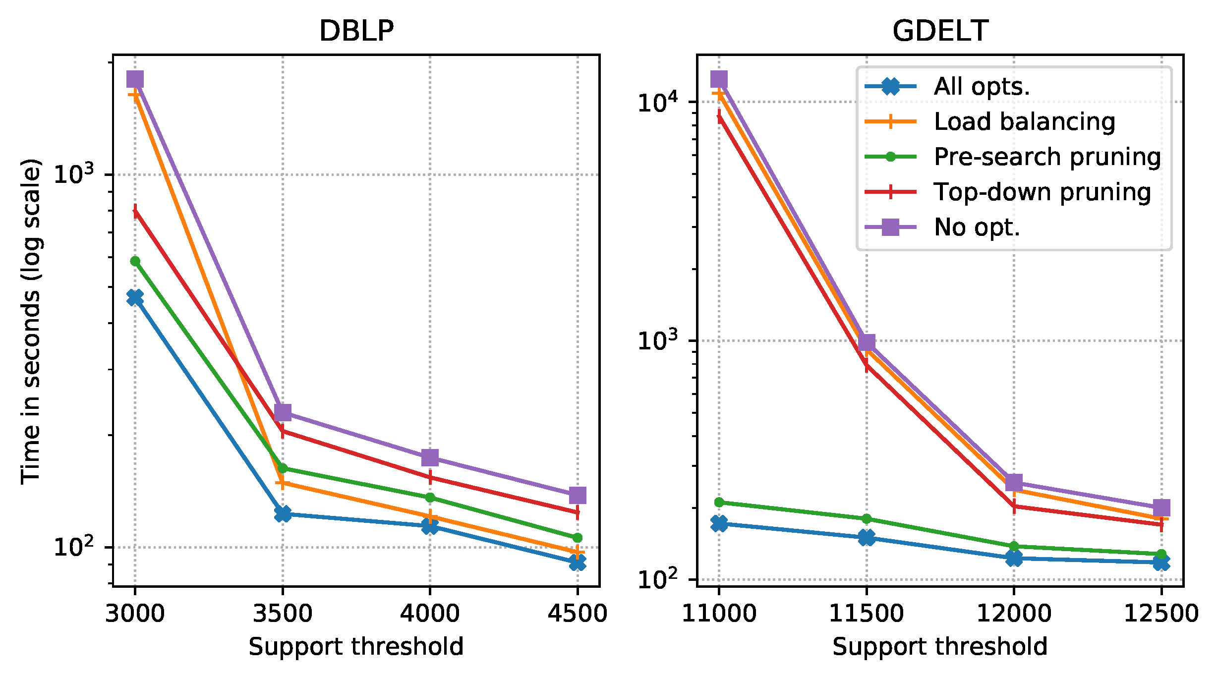
Optimization: Figure 8 demonstrates the effect of the three optimizations discussed above on the DBLP and GDELT datasets. For both datasets, the SSiGraM with all optimizations (denoted by All opts. in Figure 8) definitely performs best. For the DBLP dataset, when $\tau >3500$, load balancing is the most effective optimization while as $\tau$ becomes bigger, pre-search pruning becomes the most effective. For the GDELT dataset, the pre-pruning is always the most effective optimization. When no optimization is involved (denoted by No opt. in Figure 8), the algorithm performs worst. Actually, the effect of each optimization strategy varies with input graphs and different thresholds.

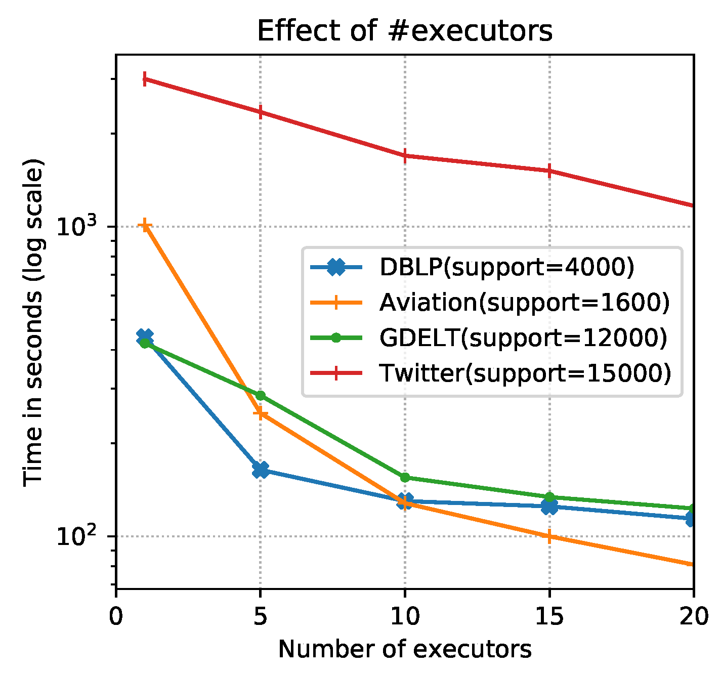
Parallelism: Finally, to evaluate the effect of the number of executors, we fix the supports of each dataset and vary the num-executor parameter of the Spark configuration file. According to the principle of the same allocated memory from YARN, we set num-executors to 20, 15, 10, 5 and 1 with executor-memory being 6 GB, 8 GB, 12 GB, 24 GB and 120 GB respectively. The results shown in Figure 9 lead to three major observations. First, compared with GraMi’s performance shown in Figure 7, the proposed algorithm outperforms the GraMi algorithm even when only one executor was used. This is because the complexity of SSGraMi is less than that of GraMi ( $\mathcal{O}(n·N^{n-1})$ ), especially when n is large. Second, the runtime decreases with the increment of parallelism for each dataset overall. Third, when the num-executor is bigger than 10, the performance improvement is less obvious because the final performance will be dependent on a few time-consuming subgraphs. Thus, most executors will wait until these subgraphs are finished. More executors cannot avoid this phenomenon.

5. Conclusions

In this paper, we propose SSiGraM, a novel parallel frequent subgraph mining algorithm in a single large graph using Spark, which conducts in parallel subgraph extension and support counting, respectively, focusing on the two core steps with high computational complexity in frequent subgraph mining. In addition, we also provide a heuristic search strategy and three optimizations for the support computing operation. Finally, extensive experimental performance evaluations are conducted with four graph datasets, showing the effectiveness of the proposed SSiGraM algorithm.

Currently, the parallel execution is conducted on the scale of every generated subgraph. When a subgraph involves a node with very big degree, SSiGraM will not go to next iteration until the executor finishes calculating the support of this subgraph. In the future, we plan to design a strategy that decomposes the evaluation task for this type of subgraph to all executors, accelerating the search speed further.

6. Discussion

The proposed algorithm in this paper is applied to FSM on a single large certain graph data, in which each edge definitely exists. However, uncertain graphs are also common and have practical importance in the real world, e.g., the telecommunication or electrical networks. In the uncertain graph model [33], each edge of a graph is associated with a probability to quantify the likelihood that this edge exists in the graph. Usually the existence of edges is assumed to be independent.

There are also two types of FSM on uncertain graphs: transaction based and single graph based. Most existing work on FSM on uncertain graphs is developed on transaction settings, i.e., multiple small/medium uncertain graphs. FSM on uncertain graph transactions under expected semantics considers a subgraph frequent if its expected support is greater than the threshold. Representative algorithms include Mining Uncertain Subgraph patterns (MUSE) [34], Weighted MUSE (WMUSE) [35], Uncertain Graph Index(UGRAP) [36] and Mining Uncertain Subgraph patterns under Probabilistic semantics (MUSE-P) [37]. They are proposed under expected semantics or the probabilistic semantics. Here, we mainly discuss the measurement of uncertainty and applications of techniques proposed in this paper considering single uncertain graph.

The measurement of uncertainty is important when considering an uncertain graph. Combining labelled graph in Definition 1 in this paper, an uncertain graph is a tuple $G^u=(G,P)$, where G is the backbone labelled graph, and $P:E\to (0,1]$ is a probability function that assigns each edge e with an existence probability, denoted by $P\left(e\right),e\in E$. An uncertain graph $G^u$ implies $2^{\left|E\right|}$ possible graphs in total, each of which is a structure $G^u$ may exist as. The existence probability of $G^i$ can be computed by the joint probability distribution:

$$P(G^u\Rightarrow G^i)=\prod _{e\in E_{G^i}}P\left(e\right)\prod _{e\in E_G/E_{G^i}}(1-P\left(e\right)).$$

Generally speaking, FSM on single uncertain graph can also be divided into two phases: subgraph extension and support evaluation. The subgraph extension phase is the same as that for FSM on the backbone graph G. Thus, techniques used in this paper, such as canonical adjacency matrix for representing subgraphs and the parallel extension for extending subgraphs, can be used in the single uncertain graph.

The biggest difference lies in the support evaluation phase. The support of a subgraph g in an uncertain graph $G^u$ is measured by expected support. A straightforward procedure to compute the expected support is generating all implied graphs, computing and aggregating the support of the subgraph in every implied graph, and last deriving the expected support, which can be accomplished by the CSP model used in this paper. Formally, the expected support is a probability distribution over the support in implied graphs:

$$eSup(g,G^u)=\sum _{i=1}^{2^{\left|E\right|}}P(G^u\Rightarrow G^i)·Sup(g,G^i),$$

where $G^i$ is an implied graph of $G^u$. The support measure $Sup$ can be the MNI support introduced in Definition 5, which is computed efficiently. Thus, given an uncertain graph $G^u=(G,P)$ and an expected support threshold $\tau$, FSM on an uncertain graph finds all subgraphs g whose expected support is no less than the threshold, i.e., $G=\left\{g\right|eSup(g,G^u)\ge \tau \wedge g\subseteq G\}$.

Furthermore, let $P_j(g,G^u)$ denote the aggregated probability that the support of g in an implied graph is no less than j:

$$P_j(g,G^u)=\sum _{G^i\in {\Delta }_j\left(g\right)}P(G^u\Rightarrow G^i),$$

where ${\Delta }_j\left(g\right)=\left\{G^i\right|Supg,G^i\ge j\}$. The expected support can be reformulated as:

$$eSup(g,G^u)=\sum _{j=1}^{M_s}{P}_j(g,G^u),$$

where $M_s$ is the maximum support of g among all implied graphs of $G^u$. For the detailed proof, we refer to [25]. However, it is #P-hard to compute $eSup(g,G^u)$ because of the huge number of implied graphs ($2^{\left|E\right|}$), which means that it is rather time consuming to draw exact frequent subgraph results even using the parallel evaluation with Spark platform proposed in this paper. Approximate evaluation with an error tolerance to allow some false positive frequent subgraphs is a common method. Some special optimization techniques other than optimizations in this paper must also be designed. Therefore, the modifications of expected support and some potential optimizations are still problems to be further studied to make the proposed algorithm be fit to mine frequent subgraphs on single uncertain graph.

References

- Chakrabarti, D.; Faloutsos, C. Graph mining: Laws, generators, and algorithms. ACM Comput. Surv. (CSUR) 2006, 38, 2. [Google Scholar] [CrossRef]
- Yan, X.; Han, J. gSpan: Graph-based substructure pattern mining. In Proceedings of the 2002 IEEE International Conference on Data Mining (ICDM 2002), Maebashi City, Japan, 9–12 December 2002; pp. 721–724. [Google Scholar]
- Liu, Y.; Xu, S.; Duan, L. Relationship Emergence Prediction in Heterogeneous Networks through Dynamic Frequent Subgraph Mining. In Proceedings of the 23rd ACM International Conference on Information and Knowledge Management, Shanghai, China, 3–7 November 2014; ACM: New York, NY, USA, 2014; pp. 1649–1658. [Google Scholar]
- Herrera-Semenets, V.; Gago-Alonso, A. A novel rule generator for intrusion detection based on frequent subgraph mining. Ingeniare Rev. Chil. Ing. 2017, 25, 226–234. [Google Scholar] [CrossRef]
- Qiao, F.; Wang, H. Computational Approach to Detecting and Predicting Occupy Protest Events. In Proceedings of the 2015 International Conference on Identification, Information, and Knowledge in the Internet of Things (IIKI), Beijing, China, 22–23 October 2015; pp. 94–97. [Google Scholar]
- Pak, A.; Paroubek, P. Extracting Sentiment Patterns from Syntactic Graphs. In Social Media Mining and Social Network Analysis: Emerging Research; IGI Global: Hershey, PA, USA, 2013; pp. 1–18. [Google Scholar]
- Choi, C.; Lee, Y.; Yoon, S.E. Discriminative subgraphs for discovering family photos. Comput. Vis. Media 2016, 2, 257–266. [Google Scholar] [CrossRef]
- Keneshloo, Y.; Cadena, J.; Korkmaz, G.; Ramakrishnan, N. Detecting and forecasting domestic political crises: A graph-based approach. In Proceedings of the 2014 ACM Conference on Web Science, Bloomington, IN, USA, 23–26 June 2014; ACM: New York, NY, USA, 2014; pp. 192–196. [Google Scholar]
- Jiang, C.; Coenen, F.; Zito, M. A survey of frequent subgraph mining algorithms. Knowl. Eng. Rev. 2013, 28, 75–105. [Google Scholar] [CrossRef]
- Kuramochi, M.; Karypis, G. Finding Frequent Patterns in a Large Sparse Graph. Data Min. Knowl. Discov. 2005, 11, 243–271. [Google Scholar] [CrossRef]
- Berlingerio, M.; Bonchi, F.; Bringmann, B.; Gionis, A. Mining graph evolution rules. In Machine Learning and Knowledge Discovery in Databases; MIT Press: Cambridge, MA, USA, 2009; pp. 115–130. [Google Scholar]
- Elseidy, M.; Abdelhamid, E.; Skiadopoulos, S.; Kalnis, P. GraMi: Frequent Subgraph and Pattern Mining in a Single Large Graph. Proc. VLDB Endow. 2014, 7, 517–528. [Google Scholar] [CrossRef]
- Wang, K.; Xie, X.; Jin, H.; Yuan, P.; Lu, F.; Ke, X. Frequent Subgraph Mining in Graph Databases Based on MapReduce. In Advances in Services Computing, Proceedings of the 10th Asia-Pacific Services Computing Conference (APSCC 2016), Zhangjiajie, China, 16–18 November 2016; Springer: Berlin, Germany, 2016; pp. 464–476. [Google Scholar]
- Liu, Y.; Jiang, X.; Chen, H.; Ma, J.; Zhang, X. Mapreduce-based pattern finding algorithm applied in motif detection for prescription compatibility network. In Advanced Parallel Processing Technologies; Springer International Publishing AG: Cham, Switzerland, 2009; pp. 341–355. [Google Scholar]
- Shahrivari, S.; Jalili, S. Distributed discovery of frequent subgraphs of a network using MapReduce. Computing 2015, 97, 1101–1120. [Google Scholar] [CrossRef]
- Aridhi, S.; d’Orazio, L.; Maddouri, M.; Nguifo, E.M. Density-based data partitioning strategy to approximate large-scale subgraph mining. Inf. Syst. 2015, 48, 213–223. [Google Scholar] [CrossRef]
- Hill, S.; Srichandan, B.; Sunderraman, R. An iterative mapreduce approach to frequent subgraph mining in biological datasets. In Proceedings of the ACM Conference on Bioinformatics, Computational Biology and Biomedicine, Orlando, FL, USA, 7–10 October 2012; ACM: New York, NY, USA, 2012; pp. 661–666. [Google Scholar]
- Luo, Y.; Guan, J.; Zhou, S. Towards Efficient Subgraph Search in Cloud Computing Environments. In Database Systems for Adanced Applications; Springer International Publishing AG: Cham, Switzerland, 2011; pp. 2–13. [Google Scholar]
- Talukder, N.; Zaki, M.J. A distributed approach for graph mining in massive networks. Data Min. Knowl. Discov. 2016, 30, 1024–1052. [Google Scholar] [CrossRef]
- White, T. Hadoop: The Definitive Guide, 1st ed.; O’Reilly Media, Inc.: Newton, MA, USA, 2009. [Google Scholar]
- Zaharia, M.; Chowdhury, M.; Franklin, M.J.; Shenker, S.; Stoica, I. Spark: Cluster Computing with Working Sets. In Proceedings of the 2nd USENIX Conference on Hot Topics in Cloud Computing (HotCloud’10), Boston, MA, USA, 22–25 June 2010; USENIX Association: Berkeley, CA, USA, 2010; p. 10. [Google Scholar]
- Meng, X.; Bradley, J.; Yavuz, B.; Sparks, E.; Venkataraman, S.; Liu, D.; Freeman, J.; Tsai, D.; Amde, M.; Owen, S.; et al. Mllib: Machine learning in apache spark. J. Mach. Learn. Res. 2016, 17, 1235–1241. [Google Scholar]
- Huan, J.; Wang, W.; Prins, J. Efficient mining of frequent subgraphs in the presence of isomorphism. In Proceedings of the Third IEEE International Conference on Data Mining (ICDM 2003), Melbourne, FL, USA, 22–22 November 2003; pp. 549–552. [Google Scholar]
- Jiang, C. Frequent Subgraph Mining Algorithms on Weighted Graphs. Ph.D. Thesis, University of Liverpool, Liverpool, UK, 2011. [Google Scholar]
- Chen, Y.; Zhao, X.; Lin, X.; Wang, Y. Towards frequent subgraph mining on single large uncertain graphs. In Proceedings of the 2015 IEEE International Conference on Data Mining (ICDM), Atlantic City, NJ, USA, 14–17 November 2015; pp. 41–50. [Google Scholar]
- Gibbons, A. Algorithmic Graph Theory; Cambridge University Press: Cambridge, UK, 1985. [Google Scholar]
- West, D.B. Introduction to Graph Theory; Prentice Hall Upper Saddle River: Bergen County, NJ, USA, 2001; Volume 2. [Google Scholar]
- Gerner, D.J.; Schrodt, P.A.; Yilmaz, O.; Abu-Jabr, R. Conflict and Mediation Event Observations (CAMEO): A New Event Data Framework for the Analysis of Foreign Policy Interactions; International Studies Association: New Orleans, LA, USA, 2002. [Google Scholar]
- He, H.; Singh, A.K. Graphs-at-a-time: Query language and access methods for graph databases. In Proceedings of the 2008 ACM SIGMOD International Conference on Management of Data, Vancouver, BC, Canada, 9–12 June 2008; ACM: New York, NY, USA, 2008; pp. 405–418. [Google Scholar]
- Fiedler, M.; Borgelt, C. Subgraph support in a single large graph. In Proceedings of the Seventh IEEE International Conference on Data Mining Workshops (ICDM Workshops 2007), Omaha, NE, USA, 28–31 October 2007; pp. 399–404. [Google Scholar]
- Bringmann, B.; Nijssen, S. What is Frequent in a Single Graph? In Proceedings of the 12th Pacific-Asia Conference on Advances in Knowledge Discovery and Data Mining (PAKDD’08), Osaka, Japan, 20–23 May 2008; Springer: Berlin/Heidelberg, Germany, 2008; pp. 858–863. [Google Scholar]
- Wörlein, M.; Meinl, T.; Fischer, I.; Philippsen, M. A quantitative comparison of the subgraph miners MoFa, gSpan, FFSM, and Gaston. In Knowledge Discovery in Database: PKDD 2005; Jorge, A., Torgo, L., Brazdil, P., Camacho, R., Gama, J., Eds.; Lecture Notes in Computer Science; Springer: Berlin, Germany, 2011; Volume 3721, pp. 392–403. [Google Scholar]
- Jin, R.; Liu, L.; Aggarwal, C.C. Discovering highly reliable subgraphs in uncertain graphs. In Proceedings of the 17th ACM SIGKDD International Conference on Knowledge Discovery and Data Mining, San Diego, CA, USA, 21–24 August 2011; ACM: New York, NY, USA, 2011; pp. 992–1000. [Google Scholar]
- Zou, Z.; Li, J.; Gao, H.; Zhang, S. Frequent subgraph pattern mining on uncertain graph data. In Proceedings of the 18th ACM Conference on Information and Knowledge Management, Hong Kong, China, 2–6 November 2009; ACM: New York, NY, USA, 2009; pp. 583–592. [Google Scholar]
- Jamil, S.; Khan, A.; Halim, Z.; Baig, A.R. Weighted muse for frequent sub-graph pattern finding in uncertain dblp data. In Proceedings of the 2011 International Conference on Internet Technology and Applications (iTAP), Wuhan, China, 16–18 August 2011; pp. 1–6. [Google Scholar]
- Papapetrou, O.; Ioannou, E.; Skoutas, D. Efficient discovery of frequent subgraph patterns in uncertain graph databases. In Proceedings of the 14th International Conference on Extending Database Technology, Uppsala, Sweden, 21–24 March 2011; ACM: New York, NY, USA, 2011; pp. 355–366. [Google Scholar]
- Zou, Z.; Gao, H.; Li, J. Discovering frequent subgraphs over uncertain graph databases under probabilistic semantics. In Proceedings of the 16th ACM SIGKDD International Conference on Knowledge Discovery and Data Mining, Washington, DC, USA, 25–28 July 2010; ACM: New York, NY, USA, 2010; pp. 633–642. [Google Scholar]
Figure 1.
(a) An event interaction graph; nodes represent the event actors (labelled with their type code) and edges represent the event (labelled with event type code); and (b,c) two subgraphs of (a) (MED: Media, REF: Refugee, GOV: Government).
Figure 2.
Minimum image (MNI) support of a subgraph -B-C-A in a single graph G with eight vertexes and three vertex labels.
Figure 3.
Three adjacency matrices , , and for the graph .
Figure 4.
Framework of the SSiGraM(Spark based Single Graph Mining) approach. Green notations on the right side are main Spark resilient distributed dataset (RDD) transformations or actions used during the algorithm pipeline. Abbreviations: CAM (Canonical Adjacency Matrix), HDFS (Hadoop Distributed File System), FFSM (Fast Frequent Subgraph Mining).
Figure 5.
Constraint satisfaction problem (CSP) search space of the subgraph with the input graph G.
Figure 6.
(a) The subgraph generation tree; and (b) the corresponding variables and domains. Marked nodes represent the pruned assignments from top to bottom.
Figure 7.
Performance of SSiGraM and GraMi on the four different datasets. Abbreviations: DBLP (DataBase systems and Logic Programming), GDELT (Global Data on Events, Location and Tone).
Figure 8.
The effect of each optimization. All opts.: All optimization enabled; Load balancing: Only load balancing enabled; Pre-pruning: Only pre-search pruning enabled; Top-down prune: Only top-down pruning enabled; No Opt.: No optimization strategies involved.
Figure 9.
The effect of the number of executors on each dataset.