Parallel Technique for the Metaheuristic Algorithms Using Devoted Local Search and Manipulating the Solutions Space


1
Institute of Mathematics, Silesian University of Technology, Kaszubska 23, 44-100 Gliwice, Poland
2
Department of Software Engineering, Kaunas University of Technology, Studentu 50, LT-51368, Kaunas, Lithuania
*
Author to whom correspondence should be addressed.
Appl. Sci. 2018, 8(2), 293; https://doi.org/10.3390/app8020293
Submission received: 16 December 2017
/
Revised: 9 February 2018
/
Accepted: 13 February 2018
/
Published: 16 February 2018
(This article belongs to the Special Issue Swarm Robotics)
Abstract
:The increasing exploration of alternative methods for solving optimization problems causes that parallelization and modification of the existing algorithms are necessary. Obtaining the right solution using the meta-heuristic algorithm may require long operating time or a large number of iterations or individuals in a population. The higher the number, the longer the operation time. In order to minimize not only the time, but also the value of the parameters we suggest three proposition to increase the efficiency of classical methods. The first one is to use the method of searching through the neighborhood in order to minimize the solution space exploration. Moreover, task distribution between threads and CPU cores can affect the speed of the algorithm and therefore make it work more efficiently. The second proposition involves manipulating the solutions space to minimize the number of calculations. In addition, the third proposition is the combination of the previous two. All propositions has been described, tested and analyzed due to the use of various test functions. Experimental research results show that the proposed methodology for parallelization and manipulation of solution space is efficient (increasing the accuracy of solutions and reducing performance time) and it is possible to apply it also to other optimization methods.
1. Introduction
Computing and operation research demand efficient methods that can increase the precision of calculations. Developments in technology provide new possibilities for faster and more efficient computing. Multi core architectures can support multi threading, where similar tasks can be forwarded to various cores for processing at the same time. This approach speeds up calculations, however it is necessary to implement a devoted methodology. Such a solution can be very useful in practical applications where many operation are made. The main target of these techniques will be, in particular, artificial intelligence (AI). AI provides many possibilities to use the power of modern computing into various applications. [1] presents a survey of modern approaches to multimedia processing. Security and communication aspects for devoted computing systems were presented in [2]. In [3], the authors presented the efficient encryption algorithm based on logistic maps and parallel technique. Moreover, parallel approach found place in medicine, especially in image processing what can be seen in [4] where lung segmentation was presented. The proposed algorithm can be used in medical support system for fast diseases detection. To create the most accurate systems that can prevent people from invisible to the eye, the initial phase of the disease. In [5], the idea of parallel solution to measurements the structural similarity between images based on quality assessment. Similar approach is present in [6], where the authors used artificial intelligence technique for image retrieval from huge medical archives.
All solutions mentioned above presented different approach to parallelization. There are various ideas to parallelize calculations, e.g. by simply performing the same task parallel on all the cores and compare the results after each iteration. Similarly we can repeat only some procedures to increase precision. However most efficient are architecture solutions designed for specific purposes. Methodology that is developed precisely for the computing task can benefit from using multi core architecture.
In recent years, various approaches to optimization problems were solved using parallel processing to increase efficiency. Photosensitive seizures were detected by application of devoted parallel methodology in [7]. The authors of [8] discussed a local search framework developed for multi-commodity flow optimization. A parallel approach to implement algorithms with and without overlapping was presented in [9]. Similarly swarm algorithms are becoming more important for optimization processes and various practical applications. In [10], the author discussed a fusion of swarm methodology with neural networks for dynamic systems simulation and positioning. Parallel implementation of swarm methodology developed for two-sided line balancing problem was discussed in [11]. Massive-passing parallel approach to implement data tests were proposed in [12]. Similarly in [13] research on efficient parallelization of dynamic programming algorithms was discussed. An extensive survey of various approaches to parallelization of algorithms with devoted platforms for classification of biological sequences was presented in [14]. While in [15] the authors discussed constraint solving algorithms in parallel versions.
Again in [16], the authors presented a combination of approximation algorithms and linear relaxation with the classical heuristic algorithm. As a result, a hybrid was obtained, which allowed to reach better results in a much shorter time. Another hybrid was shown in [17], where local search techniques were used. A similar solution has already been used in combination with the genetic algorithm, which is called the Baldwin effect [18,19]. The problem of hybridization is much widely described in [20], where there are two types of combination called collaborative (two techniques work separately and only exchange information) and integrative (one technique is built into the other). Both solutions have their own advantages and the authors pointed out them by showing ten different methodologies. The result of which is obtaining better accuracy of the solution. A particular aspect is to draw attention during modeling this type of combinations to obtain the best features of all combined components. Again in another chapter, two other types of hybridization are presented using the example of a memetic algorithm in the application of character problems. The first one considers branch and bound features within construction-based metaheuristics, and the second one branch and bound derivatives.
In this article, we present an idea for the parallelize optimization technique based on different algorithms. The proposed implementation makes use of multi core architecture by dividing calculations between all the cores, however to make the algorithm more efficient we propose also devoted way of search in the optimization space. From the basic population individuals, we select a group of best adopted ones to forward their positions for a local search in their surrounding. The local search is performed using each core and therefore the methodology benefit from faster processing but also from increased precision of calculations since during parallel mode calculations are based on the best results from each iteration. Moreover, we propose a way to divide the space due to decrease the number of possible moves for individuals in the population. Additionally, we combined both these ideas to one for greater efficiency. Our approach is different from existing one in literature not only by creating hybrids, but by dividing calculations into cores and enabling finding the best areas across the entire space. In practice, the division of space into cores is a new idea that allows not only increasing the accuracy of results but also reducing the performance time.
2. Optimization Problem and the Method of Finding the Optimal Solution
The optimization problem is understood as finding the largest or smallest value of a parameter due to certain conditions. Mathematically, the problem can be defined as follows: Let f be an objective function of n variables where and is a point. If the value of the function f at is a global minimum of the function, then is the solution. The problem of finding is called minimization problem [21]. If the value of the function at that point reaches a global minimum, then it is called a minimization problem and it can be described as
where is inequality constraint, are the boundaries of i-th variable.
For such defined problem, there is a large number of functions for which an optimal solution is hard to locate. The problem is the size of the solution space, or even the number of local extremes where the algorithm can get stacked. Some of these functions are presented in Table 1. One of the most used methods are genetic and heuristic algorithms. As heuristic, we namely algorithms that do not guarantee to find the correct solution (only the approximate) in a finite time.
2.1. Genetic Algorithm
Genetic Algorithms are examples of optimization algorithms inspired by natural selection [22]. It is a model of activities and operations on chromosomes. Algorithm assumes the creation of the beginning set of chromosomes, very often called the population. Each chromosome is presented by a binary code or a real number (more common is the second case, so we assume that). All individuals are created in a random way. Having the population, some operation are made. The first of them is the reproduction which is a process to transfer some individuals to the next operation. The most common way of reproduction is based on the probability of belonging to a particular group. In optimization problem, the group will be created by the best adapted individuals according to fitness function. The probability can be described by the following equation
where is the i-th individual in t-th iteration. For more randomness, the individual is chosen to reproduction process if it meets the following assumptions
where is the random value and is the value calculated as
So in this way, the best individuals are selected to be reproduced and it is made by two classic operators known as mutation and crossover. The first of them is understood as the modification of the chromosome by adding random value as
Of course, not every of them will be mutated – only these that will meet the inequality given as
where is mutation probability and . The second operation, which is crossover is the exchange of the information between two chromosomes and . They are called parents, and the resulting individuals as childes. The whole process can be presented as
where .
After using the described operators, all individuals in the population are evaluated by the fitness function and new population replaces the old one and it is known as succession.
The algorithm is an iterative process, so all operations are repeated until a certain number of iterations are obtained—it is presented in Algorithm 1.
| Algorithm 1: Genetic Algorithm | |
| 1: | Start, |
| 2: | Define fitness function , |
| 3: | Create an initial population, |
| 4: | Evaluate all individuals in the population, |
| 5: | Define , , and the number of iteration T, |
| 6: | , |
| 7: | while do |
| 8: | Sort individuals according to , |
| 9: | Select best individuals according to Equation (2), |
| 10: | Make a mutation by Equation (5), |
| 11: | Make a crossover using Equation (7), |
| 12: | Evaluate all new individuals in the population, |
| 13: | Replace the worst with new ones, |
| 14: | , |
| 15: | end while |
| 16: | Return the best chromosome, |
| 17: | Stop. |
2.2. Artificial Ant Colony Algorithm
Artificial Ant Colony (ACO) is an algorithm inspired by the behavior of ants. At the beginning, the algorithm was designed for discrete problems such as graph [23]. Then, different versions were designed for problems dealing with continuous functions [24]. It is a model of searching for food by ants. If the source of food is found, the ant returns to the nest leaving a pheromone trace that helps to return to the source. Unfortunately, the amount of pheromone is reduced over time due to its evaporation. The ant moves towards the selected individual from the population. The probability of selecting the j-th individual in the population is determined as
Calculating probability, a direction of movement is selected by choosing a colony c as
where is a parameter and q is random value in range and C is a random ant in population. After choosing the parent colony c, a Gaussian sampling is done. Using the density function, the scattering of pheromones in the entire space is modeled by the following equation
where is the specific coordinate for the m ant and so it is the coordinate for the selected j-th ant, and is the mean distance between the coordinate data of a points and calculated as
where is the evaporation rate.
Then, the m ant population is generated in , and the worst m individuals are deleted.
The more detailed description of ACO algorithm is presented in Algorithm 2.
| Algorithm 2: Ant Colony Optimization Algorithm | |
| 1: | Start, |
| 2: | Define fitness function , |
| 3: | Create an initial population of ants, |
| 4: | Evaluate all individuals in the population, |
| 5: | Define , n, m and the number of iteration T, |
| 6: | , |
| 7: | while do |
| 8: | for each ant do |
| 9: | Calculate the probability using Equation (8), |
| 10: | Find the best nest by Equation (9), |
| 11: | Determine Gaussian sampling according to Equation (10), |
| 12: | Create m new solutions and destroy m the worst ones, |
| 13: | end for |
| 14: | , |
| 15: | end while |
| 16: | Sort individuals according to , |
| 17: | Return the best ant, |
| 18: | Stop. |
2.3. Particle Swarm Optimization Algorithm
Particle Swarm Optimization Algorithm (PSOA) [25] is an algorithm inspired by two phenomena—swarm motion particles as well fish nebula. It describes the movement of swarm in the direction of the best individual. Despite targeted movement, the algorithm assumes randomness to increase the ability to change the best individual across the population. In order to model these phenomena, certain assumptions are introduced
- In each iteration, the number of individuals is constant,
- Only the best ones are transferred to the next iteration and the rest are randomly selected.
Each particle moves according to
where is the velocity of the i-th molecule in the t-iteration. The velocity is calculated on the basis of various factors such as the position of the best individuals in current iteration t and labeled as , which allows them to move in that direction. It is described as
where are the values chosen in random way and , are swarm controlling factors. If , all particles move in the direction of the best one. In the case when , all individuals move in random way. At the end of the iteration, only the best particles are transferred to the next iteration. The missing particles are added to population at random. The complete algorithm is presented in Algorithm 3.
| Algorithm 3: Particle Swarm Optimization Algorithm | |
| 1: | Start, |
| 2: | Define , , , number of iteration T and n, |
| 3: | Define fitness function , |
| 4: | Create an initial population, |
| 5: | , |
| 6: | while do |
| 7: | Calculate velocity using Equation (13), |
| 8: | Move each individual according to Equation (12), |
| 9: | Sort population according to , |
| 10: | Take of population to next iteration, |
| 11: | Complete the remainder of the population randomly, |
| 12: | , |
| 13: | end while |
| 14: | Return the best particle, |
| 15: | Stop. |
2.4. Firefly Algorithm
Firefly Algorithm is another mathematical model that describes the natural phenomena which is the behavior of fireflies during the searching of a parter [26]. The search is dependent on many factors such as blinking, distance or even perception by other individuals, and this introduces several factors that describes the behavior of that insects and the environment
- – light absorption coefficient,
- – coefficient of motion randomness,
- – attractiveness ratio,
- – light intensity.
A firefly moves into the most attractive individuals in the current environment based on the distance and the light intensity of a potential partner. In order to model this behavior, suppose that the distance between two individuals i and j will be be labeled as and it is calculated as
where t is the current iteration and , – k-th components of the spatial coordinates. Attractiveness between individuals is dependent on this distance – the greater the distance is, they are less attractive to each another. Moreover, the light is absorbed by the air, because of that and simplifying the model, the following assumptions are applied to the model
- Each firefly is unisex,
- The attractiveness is proportional to the brightness, which means that the less attractive firefly will move to more attractive,
- The distance is greater, the attractiveness is lower,
- If there is no attractive partner in the neighborhood, then firefly moves randomly.
Reception of light intensity from i by j decreases as the distance between them increases. Moreover, the light in nature is absorbed by different media, so attractiveness depends not only on the distance but also on absorption, so light intensity is modeled as
where is the parameter that describes light absorption mapping natural conditions of nature.
One of the assumption says that the attractiveness is proportional to the brightness (or firefly’s lightness) what is defined as
where is firefly attractiveness coefficient.
The movement of fireflies is primarily dependent on the quality of the neighborhood. The primary equation that describes that movement depends on all dependencies described above what is shown in the following formula
where is light absorption coefficient, is coefficient mapping natural randomness of fireflies, is vector defined random change of position. In each iteration, all fireflies move to find the best position according to fitness condition . Described model is presented in Algorithm 4.
| Algorithm 4: Firefly Algorithm | |
| Start, | |
| Define all coefficients and the number of iteration T and size of population, | |
| Define fitness function , | |
| Create at initial population, | |
| , | |
| while do | |
| Calculate all distances between individuals in whole population according to Equation (14), | |
| Calculate all light intensity between individuals in whole population according to Equation (15), | |
| Calculate attractiveness between individuals in whole population according to Equation (16), | |
| Evaluate and sort population, | |
| Move each firefly using Equation (17), | |
| , | |
| end while | |
| Return the best firefly, | |
| Stop. | |
2.5. Cuckoo Search Algorithm
Cuckoo Search Algorithm is another metaheuristic algorithm which stands out by gradient free optimization method [27]. It is a model that describes the behavior of cuckoos during the specific nature of breeding. These birds do not take care of theirs own eggs and throw them to other nest. So the algorithm simulates the flight while looking for nests of other birds and laying eggs in there. Of course, there is also need to pay attention to the owner’s response. In these model, some assumption must be done
- Cuckoo is identified with the egg,
- Each cuckoo has one egg,
- The nest owner decides to keep or throw the egg out with the probability . If the egg is thrown out, the new cuckoo is replace these one and the position is chosen at random.
At the beginning of the algorithm, an initial population is created in random way. Each cuckoo moves by making a flight which uses the random walk concept. It is modeled as
where is the length of random walk step with normal distribution and is Lvy flight defined as
where is the length of the step, is the minimum step for random walk and is a scaling parameter.
Once the individuals in the population have completed their movement, decide if the egg stays at the current position should be made. It is a decision-making mechanism by the owner of the nest to which the eggs were thrown. It is modeled as
where is a random value understood as the chance for egg to stay. Whole algorithm is described in Algorithm 5.
| Algorithm 5: Cuckoo Search Algorithm | |
| Start, | |
| Define all parameters , , , , , number of and iterations T, | |
| Define fitness function , | |
| Create an initial population, | |
| t:=0, | |
| while do | |
| Move individuals to another position using Equations (18) and (19), | |
| According to Equation (20), the nest host decides whether the cuckoo eggs remain, | |
| Evaluate the whole population, | |
| Sort the population according to fitness condition, | |
| , | |
| end while | |
| Return the best cuckoo, | |
| Stop. | |
2.6. Wolf Search Algorithm
One of the new heuristic algorithms is Wolf Search Algorithm described for the first time in [28]. In the algorithm, the behavior of wolves during the search for food and avoid other predators is modeled. The model assumes that the wolf can only see in a certain area around himself and he can only move in it. This area is understood as a circle, where the center is the point (wolf) with r radius. The wolf’s position is assessed in terms of its adaptability to the function which values are interpreted as a number of food locations in the circle. There is a situation that the wolf quickly escapes outside this area when another predator is in the vicinity or the amount of food in the area is quite low.
Such a behavior of the wolf while searching for food is modeled for optimization purposes. Let be a particular wolf among the whole population. The actual position of will be designated as . Wolf moves according to
where is the ultimate incentive, is the closest neighbor with higher value of fitness function, is random number in and r means the distance between two wolves and calculated as the Euclidean metric already described in Equation (14). Wolf moves by Equation (21), when he spotted a better feeding. Otherwise, the wolf tries to hunt. Hunting of wolves lies in a process of stalking that can be represented into three steps
- initiative stage – wolf moves in the area of his vision and looks for food. This behavior is modeled by changing the position of the wolf in the following waywhere v is the velocity of a wolf.
- passive stage – wolf waits for the opportunity to attack on a given position and tries to attack by Equation (21).
- escape – in case of lack of food or the appearance of another predator, the wolf escapes bywhere k is the step size.
It is simply model showing the behavior of wolves. In each iteration, wolves search for better food source and in the end, the wolves that is identified with best food source is the result. The full algorithm is presented in Algorithm 6.
| Algorithm 6: Wolf Search Algorithm | |
| Start, | |
| Define basic parameters of the algorithm – the number of iterations T, the number of wolves n, radius of view r, step size k, velocity coefficient and rate of appearance of the enemy , | |
| Generate a population of wolves at random, | |
| , | |
| while do | |
| for each wolf in population do | |
| Check the viewing area by Equation (22), | |
| Calculate the new position using Equation (21), | |
| if then | |
| Move the wolf from to , | |
| end if | |
| Select the value of the parameter at random, | |
| if then | |
| The wolf performs escape by Equation (23), | |
| end if | |
| end for | |
| , | |
| end while | |
| Return the fittest wolf in the population, | |
| Stop. | |
3. Manipulation of Swarms Positions and Space Solution Using Multi-Threaded Techniques
The problem of finding the optimal solution is more difficult if the test function is complicated. As complicated we understand the function of which extremes are hard to locate by classical methods. In this case, the application of meta–heuristic methodology seems to be a good solution. However, in some cases the values of the parameters should be significantly increased like the number of individuals in a population as well as the number of iterations. Increasing the value of these parameters increases the number of performed operations and thus action time. In addition, these algorithms do not guarantee the correct solution. With these problems, the application of these techniques may prove to be very detrimental.
3.1. Proposition I
In order to minimize the amount of computation time, we suggest using automatic parallelization of the algorithms by dividing the population into several groups, which threads are burdened.
From the perspective of nature, individuals analyze the environment and choose the best of them all. In the neighborhood of the best solution, smaller populations called groups may be formed. Suppose that at the beginning of the algorithm, the number of cores is detected. In analogy to the original version of the algorithms, an initial population consisting of n individuals is created at random. From this population, fittest individuals are chosen. Each individual will be the best adapted solution in the smaller group that will be created under his leadership. The size of the group will be determined as follows
The above equation uses the floor to obtain groups with the same population size for each core. The use of the floor guarantees that, regardless of n, each group will have the same number of individuals, and the sum of all will not exceed n.
With the size of the group and their leadership, we can begin to create groups. For every alpha male, we create one thread on which the population consisting of individuals is created. Each individual in the group is placed in a random way at a distance of no more than from the leader. This distance can be calculated by
where a, b are the values of the variable’s range for the test function.
For each group on a separate thread, all steps from an original algorithms are performed. After completing these steps, the best adapted individuals are found as a solution for the optimization problem and selected the best of them. Complete operation of the proposed method is shown in Algorithm 7.
| Algorithm 7: Metaheuristic with devoted local search |
|
3.2. Proposition II
In the previously proposition, we proposed a technique for putting individuals in a given population on the solution space and assigning them a thread for calculation. Another way to increase the efficiency is to manipulating the solution space in such a way as to limit the possibility of movements in the least favorable areas. Imagine that in the early iterations of the algorithm, the population begins to move in the best areas, i.e., an area where the extreme may potentially occur. Suppose that we have processor cores, so threads can be created. Our solution space for fitness function f can be presented as
where are values that divide the set into such two subsets , that Equation (26) is satisfied and × means Cartesian product (note that the limit values and correspond to a and b). Using that information, we can divide this space into smallest intervals as
Taking these small intervals and use them to describe the solution space for function f would be
Unfortunately, these formulations give us parts of solution space. The reason for that is dividing each side of the interval on parts. Having only cores, it is necessary to merge some areas to obtain exactly number of . To do that, we can describe formula for vertical merge of areas for specific cores—for first one as
and for each subsequent m core as
Let us prove, that sum of all these parts are equal to the initial solution space.
Proof.
Taking all areas dedicated for first core described in Equation (29), we have
the same is done with the rest areas in Equation (30) as
By adding sets obtained above, we have
☐
This gives the areas (making the whole solutions space). Now, for each core, of the entire size of the population n is created ()—but the individuals are made in the selected area, not in the whole space. After of all iteration t, each core k is evaluated as
where and they are coefficients describing the importance of a given part – the average of all individuals and the best individual on the current thread. We choose the p best areas and repeated the movement of population on each core in the sum of these areas by of the iteration and of the individuals. If the case, when individuals leaves the area, he is killed and a new individual is created in his place. After all iteration, the best solution is funded in all populations.
In this proposition, the multi-threading technique has a big role because dividing the space and choosing the best areas does not cost extra time and above all, it allows the placement of most individuals in a smaller area in parallel several times. These actions are described in Algorithm 8
| Algorithm 8: Analysis of the solution space for the initial population |
|
3.3. Proposition III
Our last proposition is the combination of the above two propositions with some modifications. At first, we dividing solution space according to (29) and (30). Having the number of areas, threads can be created. of all individuals are created in each area for iterations. The occurring for iterations and populations may have different values. To simplify the introduction of a large number of parameters, we assume that they have the same value. At the end, in each population, the best individuals stays, the rest of them is destroyed.
For each survived individual (which are identify with the best solutions), a group is formed exactly like in Section 3.1 but the size of group should not be greater than of all n. Next, all individuals moves for the rest of iterations. In addition, then, the population size is replenished (if the size is smaller than n) in a random way throughout the area.
4. Test Results
All presented propositions have been implemented along with extended versions with the proposed multi–threading technique. All tests were carried out on the six-processor Intel Core i7 6850K clocked at GHz.
4.1. The Benchmark Functions
Proposed solutions were tested on different 10 functions described in Table 1. All these functions were given in dimension . The selected functions are the representatives of different types like bowl, plate, valley shaped and with many local minima.
4.2. Experimental Settings
In experiments, we used described version of classical meta–heuristic algorithms. For all tests, we used the same numbers of iterations and population size of 100 individual and . For each test, 100 measurements were taken and averaged. The tests were performed in terms of performance depending on the number of cores and as regards the accuracy of averaged solutions.
The coefficients used by all the algorithm have been selected before the start of operation. The influence of the increase in coefficients values causes the multitude of a given step or displacement of individuals. Therefore, in our considerations we do not analyze the impact of these coefficients on the method and accuracy of the obtained solutions, and each parameter was chosen in a random way in the range . The obtained values of coefficients were respectively
- Genetic algorithm – ,
- Ant Colony Optimization Algorithm – , , ,
- Particle Swarm Optimization Algorithm – , , ,
- Firefly Algorithm – , ,
- Cuckoo Search Algorithm – , , , , ,
- Wolf Search Algorithm – , , .
4.3. Performance Metrics
For the purpose of evaluating algorithms, several basic metrics have been used. The accuracy of the optimization algorithms is evaluated by the average value of the solution obtained from the tests carried out what can be presented as
and error calculated as an absolute value between the ideal and obtained solution which is
The second aspect is parallelization evaluated by two metrics – acceleration and efficiency . Acceleration is the ratio of sequential execution time of the algorithm defined as
where is execution time measured for one processor, and is execution time measured for processors. The second assessment is made by the following formula
In addition, scalability with the number of cores is measured in accordance with Amdahl’s law
where is the proportion of execution time of the proposal to the original versions. For our measurements, was determined as the quotient of the average time for all algorithms for cores and the sum of time needed for and one processor.
4.4. Results
Firstly, we analyzed the impact of different coefficient values on the algorithms. We noticed that the coefficient values depend on the function itself—the more local extremes, the higher the values should be. This is due to the fact that individuals have to get out in such a minimum location, hence the large values of coefficients can prolong movement in one iteration and allow escape. Such reasoning forced us to depend on the value of coefficients from the pseudorandom generator. This action, combined with averaging the obtained results, enabled to obtain averaged solutions. It was performed for all versions of the algorithms—the original and three proposed modifications in this paper. The obtained solution are presented in Table 2, Table 3, Table 4 and Table 5 and errors values are in Table 6, Table 7, Table 8 and Table 9. In all cases, the first proposition—the use of devoted local search—reduced the error values in almost every case. Of course, there were cases when the selected algorithms had a minimal difference between the results (see CSA results), although it may be due to bad initial position of individuals. In contrast, the second proposal related to the division of the solution space brought quite a big drop in the value of errors for each case. This points to the fact that the size of the space is very important for metaheuristics—a search of the same area in less time and without necessarily increasing computing needs is a very important issue. The proposed division of space is one of the many cases that can be corrected, but it is one that significantly improves solution for each test function indicates the direction of future research. Moreover, the combination of these two proposition improved the obtained results for many cases, but not for all. GA and PSOA improved solutions for more than 5 cases, when FA improved the score for 9 from 10 benchmark functions. For better visualization the error values, The average error obtained for each version of the algorithm is shown in Figure 1. The graph shows that the error value is the smallest when applying proposition 2 or 3, and 1 has an approximately constant error.
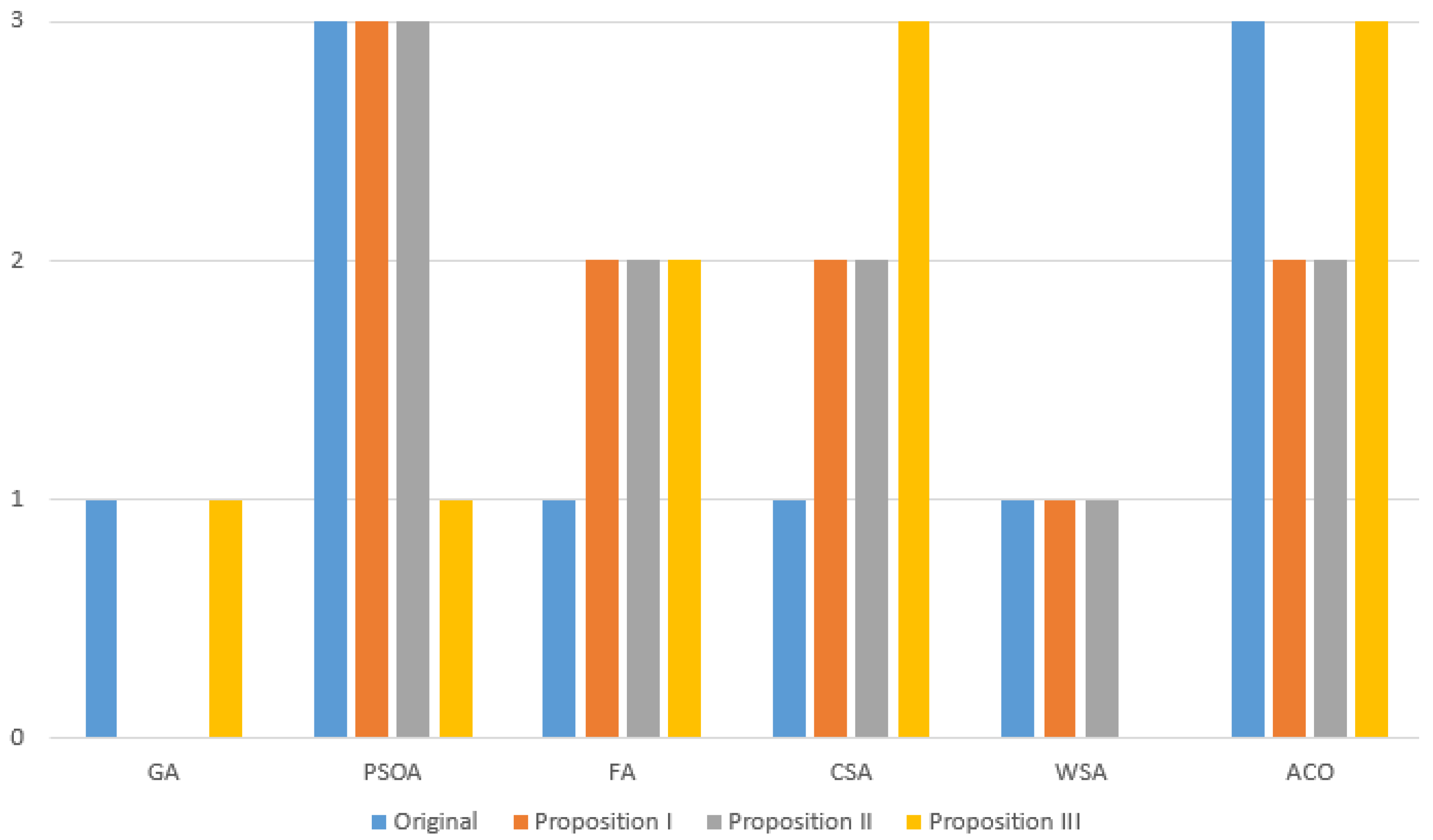
We also evaluated individual algorithms by assigning them ranks for each proposal—if the algorithm obtained the most accurate solution for a given function using a particular technique, it received one point. Results are presented in Figure 2, and it is easy to notice that depending on the chosen proposal, another algorithm proved to be the best. It is easy to notice that depending on the chosen proposal, another algorithm proved to be the best. Without any modification the best algorithm was classic version of PSOA and ACO. Adding first proposition the best one were PSOA and FA, CSA, ACO are in the second place equally, and with second proposals, there are the same scores. The third modification allowed CSA and ACO to be the best algorithms. Of course, obtained results depend on the equations of motion, their length and other factors affecting such a large palette of metaheuristic methods. Not only, the accuracy was measured, but the duration of action with using multithreading techniques. Measured time values are presented in Table 4, Table 10, Table 11, Table 12, Table 13 and on Figure 3. The use of any modification shortens the operating time for almost every case compared to the original versions. What is interesting, first and second proposition shortened time of approximately the same value, when the third obtained the best result in this aspect. To accurately assess the operation time, we used the formulas described in Equations (37) and (38), the obtained results are presented in Table 14. The worst results were achieved for the first modification, than the third one and the second one as the best one in terms of acceleration. Scalability for each proposition (having 6 cores) were approximately successively , and . To analyze these values, we also calculated the scalability for the 2 and 4 cores which results are presented in Figure 4. Ideal solution would be linear curve, but the more cores are used, the worst scalability is. In the case of the first two proposals, it decreases quite rapidly. However, the scalability of proposition III only minimally decreases after using more than 4 cores. Another aspect is the number of iteration needed for the sequential version to get similar results (approximately) to the presented proposals. The obtained data are presented in Table 15. In the case of 6 cores (for proposition I and II), the number of iteration must be increased by almost 22–26%. Such a large discrepancy is caused by the randomness of the algorithms (for example, the initial distribution of the population). In the case of proposals III, the sequential algorithm needs about more iterations.
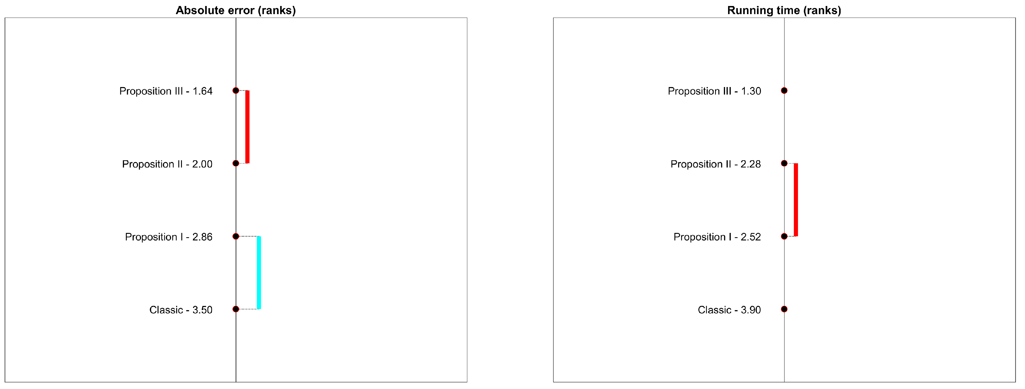
A factorial ANOVA test was conducted to compare the main effects of absolute error and running time values among classic meta-heuristic and three proposed techniques. The results was significant both for absolute error and running time . The results of Friedman-Nemenyi tests of ranking further reveal that the performance of Proposition III is the best among all techniques in terms absolute error (, critical distance ; tied with Proposition II) and running time (, critical distance ). The ranks of the methods within the critical distance are not significantly different (see Figure 5). The results are confirmed by the random permutation test (10000 permutations). Proposition III has lower absolute error than Classic method (), Proposition I (), and Proposition II (). Proposition III has lower running time than Classic method (), Proposition I (), and Proposition II ().
5. Conclusions
In this paper, we described six, classic meta–heuristic algorithms designed for optimization purposes and proposed three techniques for increasing not only the accuracy, but also the efficiency of the operation. Our ideas were based primarily on the action of multi–threading, which allowed placing individuals of a given population in specific places where an extreme can be located. An additional idea was to divide and manipulate the solutions space, which is interpreted as the natural environment of the individuals in given population. These types of activities have been tested and analyzed in terms of average error for selected functions and the time needed to perform the calculations to find a solution. The obtained results indicated that each proposed modification shortens the time of operation, but not all improve (significantly) the accuracy of the obtained measurements. The high scalability of the proposal indicates that the increasing number of cores speeds up the work of modifications. Moreover, each proposition showed the acceleration of the performance time as well as increasing the accuracy of the obtained solutions regardless of the chosen heuristic algorithm.
While the proposed techniques of parallelization and manipulation of solution space have improved the operation of classical algorithms, they are so flexible that can be streamlined and improved by various ideas. In addition, this can allow to obtain even better results. This paper gives only an example of the parallelization approach. It seems reasonable to divide the search space in such a way that the area given to one particular core will be contained in the next and subsequent one. In addition, a model of communication between populations would be needed to exchange information about unfavorable areas. This would allow them to be removed from space and extended to another area on each core. In practice, this will eliminate unnecessary searches of uninteresting places, and at the same time increase precision (allowing individuals to move around in better places) and reduce computation time due to the reduction of the area on all cores.
Acknowledgments
Authors acknowledge contribution to this project to the Diamond Grant No. 0080/DIA/2016/45 funded by the Polish Ministry of Science and Higher Education and support from Software Engineering Department at Kaunas University of Technology, Lithuania.
Author Contributions
Dawid Połap, Karolina Kęsik, Marcin Woźniak and Robertas Damaševičius designed the methods, performed experiments and wrote the paper.
Conflicts of Interest
The authors declare no conflict of interest.
References
- Shaoping, L.; Taijiang, M.; Zhang, S. A survey on multiview video synthesis and editing. Tsinghua Sci. Technol. 2016, 21, 678–695. [Google Scholar]
- Hong, Z.; Jingyu, W.; Jie, C.; Shun, Z. Efficient conditional privacy-preserving and authentication scheme for secure service provision in vanet. Tsinghua Sci. Technol. 2016, 21, 620–629. [Google Scholar]
- Rostami, M.; Shahba, A.; Saryazdi, S.; Nezamabadi-pour, H. A novel parallel image encryption with chaotic windows based on logistic map. Comput. Electr. Eng. 2017, 62, 384–400. [Google Scholar] [CrossRef]
- MY, S.T.; Babu, S. An intelligent system for segmenting lung image using parallel programming. In Proceedings of the International Conference on Data Mining and Advanced Computing (SAPIENCE), Ernakulam, India, 16–18 March 2016; Volume 21, pp. 194–197. [Google Scholar]
- Lan, G.; Shen, Y.; Chen, T.; Zhu, H. Parallel implementations of structural similarity based no-reference image quality assessment. Adv. Eng. Softw. 2017, 114, 372–379. [Google Scholar] [CrossRef]
- Khatami, A.; Babaie, M.; Khosravi, A.; Tizhoosh, H.R.; Nahavandi, S. Parallel Deep Solutions for Image Retrieval from Imbalanced Medical Imaging Archives. Appl. Soft Comput. 2017, 63, 197–205. [Google Scholar] [CrossRef]
- Alzubaidi, M.; Otoom, M.; Al-Tamimi, A.K. Parallel scheme for real-time detection of photosensitive seizures. Comput. Biol. Med. 2016, 70, 139–147. [Google Scholar] [CrossRef] [PubMed]
- Munguía, L.; Ahmed, S.; Bader, D.A.; Nemhauser, G.L.; Goel, V.; Shao, Y. A parallel local search framework for the fixed-charge multicommodity network flow problem. Comput. OR 2017, 77, 44–57. [Google Scholar] [CrossRef]
- Gomis, H.M.; Migallón, V.; Penadés, J. Parallel alternating iterative algorithms with and without overlapping on multicore architectures. Adv. Eng. Softw. 2016, 10, 27–36. [Google Scholar]
- Woźniak, M.; Połap, D. Hybrid neuro-heuristic methodology for simulation and control of dynamic systems over time interval. Neural Netw. 2017, 93, 45–56. [Google Scholar] [CrossRef] [PubMed]
- Tapkan, P.; Özbakir, L.; Baykasoglu, A. Bee algorithms for parallel two-sided assembly line balancing problem with walking times. Appl. Soft Comput. 2016, 39, 275–291. [Google Scholar] [CrossRef]
- Tian, T.; Gong, D. Test data generation for path coverage of message-passing parallel programs based on co-evolutionary genetic algorithms. Autom. Softw. Eng. 2016, 23, 469–500. [Google Scholar] [CrossRef]
- Maleki, S.; Musuvathi, M.; Mytkowicz, T. Efficient parallelization using rank convergence in dynamic programming algorithms. Commun. ACM 2016, 59, 85–92. [Google Scholar] [CrossRef]
- De Oliveira Sandes, E.F.; Maleki, S.; Musuvathi, M.; Mytkowicz, T. Parallel optimal pairwise biological sequence comparison: Algorithms, platforms, and classification. ACM Comput. Surv. 2016, 48, 63. [Google Scholar]
- Truchet, C.; Arbelaez, A.; Richoux, F.; Codognet, P. Estimating parallel runtimes for randomized algorithms in constraint solving. J. Heuristics 2016, 22, 613–648. [Google Scholar] [CrossRef]
- D’Andreagiovanni, F.; Krolikowski, J.; Pulaj, J. A fast hybrid primal heuristic for multiband robust capacitated network design with multiple time periods. Appl. Soft Comput. 2015, 26, 497–507. [Google Scholar] [CrossRef]
- Gambardella, L.; Luca, M.; Montemanni, R.; Weyland, D. Coupling ant colony systems with strong local searches. Eur. J. Oper. Res. 2012, 220, 831–843. [Google Scholar] [CrossRef]
- Whitlay, D.; Gordon, V.; Mathias, K. Lamarckian evolution, the Baldwin effect and function optimization. In Proceedings of the International Conference on Parallel Problem Solving from Nature, Jerusalem, Israel, 9–14 October 1994; pp. 5–15. [Google Scholar]
- Woźniak, M.; Połap, D. On some aspects of genetic and evolutionary methods for optimization purposes. Int. J. Electr. Telecommun. 2015, 61, 7–16. [Google Scholar] [CrossRef]
- Blum, C.; Roli, A.; Sampels, M. Hybrid Metaheuristics: An Emerging Approach to Optimization; Springer: Berlin/Heidelberg, Germany, 2008. [Google Scholar]
- Luenberger, D.G.; Ye, Y. Linear and Nonlinear Programming; Springer: Berlin/Heidelberg, Germany, 1984. [Google Scholar]
- Lawrence, D. Handbook of Genetic Algorithms; Van Nostrand Reinhold: New York, NY, USA, 1991. [Google Scholar]
- Dorigo, M.; Gambardella, L.M. Ant colony system: A cooperative learning approach to the traveling salesman problem. IEEE Trans. Evolut. Comput. 1997, 1, 53–66. [Google Scholar] [CrossRef]
- Ojha, V.K.; Ajith, A.; Snášel, V. ACO for continuous function optimization: A performance analysis. In Proceedings of the 14th International Conference on Intelligent Systems Design and Applications (ISDA), Okinawa, Japan, 28–30 November 2014; pp. 145–150. [Google Scholar]
- Clerc, M. Particle Swarm Optimization; John Wiley & Sons: Hoboken, NJ, USA, 2010. [Google Scholar]
- Yang, X.-S. Firefly algorithm, stochastic test functions and design optimization. Int. J. Bio-Inspir. Comput. 2010, 2, 78–84. [Google Scholar] [CrossRef]
- Yang, X.-S.; Deb, S. Cuckoo search via Lévy flights. In Proceedings of the NaBIC 2009 World Congress on Nature & Biologically Inspired Computing, Coimbatore, India, 9–11 December 2009; pp. 210–214. [Google Scholar]
- Rui, T.; Fong, S.; Yang, X.; Deb, S. Wolf search algorithm with ephemeral memory. In Proceedings of the Seventh IEEE International Conference on Digital Information Management (ICDIM), Macau, Macao, 22–24 August 2012; pp. 165–172. [Google Scholar]
Figure 1.
The average error obtained for each version of the algorithm.

Figure 2.
The performance ranking of tested algorithms—the number of times the algorithm ranked first.
Figure 2.
The performance ranking of tested algorithms—the number of times the algorithm ranked first.

Figure 3.
Comparison of the average time needed to find the optimum for 100 individuals during 100 iterations for 100 tests for each algorithm and all tested versions.
Figure 3.
Comparison of the average time needed to find the optimum for 100 individuals during 100 iterations for 100 tests for each algorithm and all tested versions.

Figure 4.
Scalability for each proposition.

Figure 5.
The results of Friedman-Nemenyi tests of ranking.


Table 1.
Test functions used in a minimization problem.
| Function Name | Function f | Range | Solution | |
|---|---|---|---|---|
| Dixon-Price | 0 | |||
| Griewank | 0 | (0,…,0) | ||
| Rotated Hyper–Ellipsoid | 0 | (0,…,0) | ||
| Schwefel | 0 | (420.97,…,420.97) | ||
| Shubert | (0,…,0) | |||
| Sphere | 0 | (0,…,0) | ||
| Sum squares | 0 | (0,…,0) | ||
| Styblinski-Tang | (,…,) | |||
| Rastrigin | 0 | (0,…,0) | ||
| Zakharov | 0 | (0,…,0) |
Table 2.
Averaged solution values achieved by all original algorithms for each test functions.
| Function | GA | PSOA | FA | CSA | WSA | ACO |
|---|---|---|---|---|---|---|
| 0.07593 | 0.08617 | 0.26872 | 0.16432 | 0.00257 | 0.00319 | |
| 0.12283 | 0.16489 | 0.18691 | 0.1729 | 0.1275 | 0.13129 | |
| 0.00172 | 0.27991 | 0.05206 | 0.00948 | 0.00029 | 0.00192 | |
| 0.00506 | 0.00963 | 0.00174 | 0.01354 | 0.00981 | 0.00166 | |
| −185.843 | ||||||
| 0.00001 | 0 | 0.00001 | 0.0002 | 0.00001 | 0.00001 | |
| 0.00105 | 0.00062 | 0.66179 | 0.00035 | 0.00025 | 0.00037 | |
| 0.19899 | 0.07731 | 0.13266 | 0.07822 | 0.1328 | 0.09898 | |
| 0.00103 | 0.00172 | 0.04368 | 0.33444 | 0.00103 | 0.00098 |
Table 3.
Averaged solution values achieved by all algorithms for each test functions for proposition I.
Table 3.
Averaged solution values achieved by all algorithms for each test functions for proposition I.
| Function | GA | PSOA | FA | CSA | WSA | ACO |
|---|---|---|---|---|---|---|
| 0.05754 | 0.02098 | 0.06574 | 0.03123 | 0.16919 | 0.00317 | |
| 0.09337 | 0.10636 | 0.08035 | 0.09318 | 0.10691 | 0.08546 | |
| 0.00046 | 0.00019 | 0.01644 | 0.15137 | 0.04208 | 0.00043 | |
| 0.00083 | 0.00165 | 0.00203 | 0.00913 | 0.0002 | 0.00035 | |
| 0 | 0 | 0 | 0.00004 | 0 | 0.00053 | |
| 0.00272 | 0.00101 | 0.00023 | 0.00001 | 0.00634 | 0.00053 | |
| 9411-391 | ||||||
| 0.1072 | 0.23339 | 0.1063 | 0.98148 | 0.19899 | 0.00977 | |
| 0.00172 | 0.00006 | 0.00094 | 0.01052 | 0.00109 | 0.0015 |
Table 4.
Averaged solution values achieved by all algorithms for each test functions for proposition II.
Table 4.
Averaged solution values achieved by all algorithms for each test functions for proposition II.
| Function | GA | PSOA | FA | CSA | WSA | ACO |
|---|---|---|---|---|---|---|
| 0.03072 | 0.00027 | 0.08178 | 0.00217 | 0.0039 | 0.00032 | |
| 0.09337 | 0.07208 | 0.05691 | 0.07437 | 0.10287 | 0.06821 | |
| 0.00001 | 0 | 0 | 0.00006 | 0.00005 | 0.00002 | |
| 0.00079 | 0.00083 | 0.00166 | 0.00015 | 0.00011 | 0.00029 | |
| 0.00001 | 0 | 0.00001 | 0.00003 | 0 | 0 | |
| 0.00124 | 0.00023 | 0.00005 | 0.00002 | 0.00013 | 0.00012 | |
| 0.01592 | 0.03343 | 0.0199 | 0.00995 | 0.01 | 0.00899 | |
| 0.00314 | 0 | 0.00971 | 0.00117 | 0.00073 | 0 |
Table 5.
Averaged solution values achieved by all algorithms for each test functions for proposition III.
Table 5.
Averaged solution values achieved by all algorithms for each test functions for proposition III.
| Function | GA | PSOA | FA | CSA | WSA | ACO |
|---|---|---|---|---|---|---|
| 0.00892 | 0.00913 | 0.00088 | 0.01001 | 0.00785 | 0.00339 | |
| 0.06694 | 0.02898 | 0.00948 | 0.01298 | 0.0238 | 0.00539 | |
| 0 | 0 | 0.0001 | 0.00044 | 0.00005 | 0.00001 | |
| 0.00218 | 0.001 | 0.00012 | 0.00179 | 0.00019 | 0.00049 | |
| 0 | 0 | 0 | 0.00002 | 0 | 0 | |
| 0.00001 | 0.00007 | 0 | 0 | 0.00003 | 0.00008 | |
| 0.00996 | 0.02995 | 0.12367 | 0 | 0.03033 | 0.00139 | |
| 0.00658 | 0.00023 | 0.00014 | 0.01467 | 0.00022 | 0 |
Table 6.
Function error values achieved by all original algorithms for each test functions.
| Function | GA | PSOA | FA | CSA | WSA | ACO |
|---|---|---|---|---|---|---|
| −0.08617 | −0.16432 | −0.00257 | −0.00319 | |||
| −0.12283 | −0.16489 | −0.18691 | −0.17290 | −0.12750 | −0.13129 | |
| −0.00172 | −0.27991 | −0.05206 | −0.00948 | −0.00029 | −0.00192 | |
| −0.00506 | −0.00963 | −0.00174 | −0.01354 | −0.00981 | −0.00166 | |
| −0.68573 | −0.86850 | −0.85691 | −0.87632 | −0.89550 | −0.88475 | |
| 0 | 0 | −0.00001 | −0.00020 | 0 | 0 | |
| −0.00106 | −0.00062 | −0.66179 | −0.00035 | −0.00025 | −0.00037 | |
| −0.67100 | −0.41761 | −0.65646 | −0.25370 | −0.40180 | −0.40560 | |
| −0.33445 | −0.00103 | −0.00172 | −0.00006 | −0.00094 | −0.01052 | |
| −0.00103 | −0.00172 | −0.04368 | −0.33445 | −0.00103 | −0.00098 |
Table 7.
Averaged errors values achieved by all algorithms for each test functions for proposition I.
Table 7.
Averaged errors values achieved by all algorithms for each test functions for proposition I.
| Function | GA | PSOA | FA | CSA | WSA | ACO |
|---|---|---|---|---|---|---|
| −0.05754 | −0.02098 | −0.06574 | −0.03123 | −0.16919 | −0.00317 | |
| −0.09337 | −0.10636 | −0.08035 | −0.09318 | −0.10690 | −0.08546 | |
| −0.00046 | −0.00019 | −0.01644 | −0.15137 | −0.04208 | −0.00043 | |
| −0.00083 | −0.00165 | −0.00203 | −0.00913 | −0.00020 | −0.00035 | |
| 0.21804 | 0.37145 | 0.21421 | 0.26740 | 0.35291 | 0.28987 | |
| 0 | 0 | 0 | −0.00004 | 0 | 0 | |
| −0.00272 | −0.00101 | −0.00023 | −0.00001 | −0.00634 | −0.00053 | |
| −0.21651 | −0.17610 | −0.17057 | −0.08075 | −0.06011 | −0.05886 | |
| −0.01052 | −0.00109 | −0.00314 | 0 | −0.00971 | −0.00117 | |
| −0.00172 | −0.00006 | −0.00094 | −0.01052 | −0.00109 | −0.00150 |
Table 8.
Averaged errors values achieved by all algorithms for each test functions for proposition II.
Table 8.
Averaged errors values achieved by all algorithms for each test functions for proposition II.
| Function | GA | PSOA | FA | CSA | WSA | ACO |
|---|---|---|---|---|---|---|
| −0.03072 | −0.00027 | −0.08178 | −0.00217 | −0.00390 | −0.00032 | |
| −0.09337 | −0.07208 | −0.05691 | −0.07437 | −0.10287 | −0.06782 | |
| −0.00001 | 0 | 0 | −0.00006 | −0.00005 | −0.00002 | |
| −0.00079 | −0.00083 | −0.00166 | −0.00015 | −0.00011 | −0.00029 | |
| −0.26173 | −0.41035 | −0.10293 | −0.13672 | −0.06741 | −0.00622 | |
| 0 | 0 | 0 | −0.00003 | 0 | 0 | |
| −0.00124 | −0.00023 | −0.00005 | −0.00002 | −0.00013 | −0.00012 | |
| −0.03217 | −0.10752 | −0.01222 | −0.01671 | −0.07361 | −0.02173 | |
| −0.00117 | −0.00073 | −0.00658 | −0.00023 | −0.00014 | −0.01467 | |
| −0.00314 | 0 | −0.00971 | −0.00117 | −0.00073 | 0 |
Table 9.
Averaged errors values achieved by all algorithms for each test functions for proposition III.
Table 9.
Averaged errors values achieved by all algorithms for each test functions for proposition III.
| Function | GA | PSOA | FA | CSA | WSA | ACO |
|---|---|---|---|---|---|---|
| −0.00892 | −0.00913 | −0.00088 | −0.01001 | −0.00785 | −0.00339 | |
| −0.06694 | −0.02898 | −0.00948 | −0.01298 | −0.02380 | −0.00539 | |
| 0 | 0 | −0.00010 | −0.00044 | −0.00005 | −0.00001 | |
| −0.00218 | −0.00100 | −0.00012 | −0.00179 | −0.00019 | −0.00049 | |
| −0.00843 | −0.00147 | −0.00634 | −0.00199 | −0.00136 | 0.400033 | |
| 0 | 0 | 0 | −0.00002 | 0 | 0 | |
| −0.00001 | −0.00007 | 0 | 0 | −0.00003 | −0.00008 | |
| −0.10710 | −0.08110 | −0.00981 | −0.00009 | −0.00710 | −0.00009 | |
| −0.01467 | −0.00022 | 0 | −0.10287 | −0.06782 | −0.06694 | |
| −0.00658 | −0.00023 | −0.00014 | −0.01467 | −0.00022 | 0 |
Table 10.
Running time values achieved by all algorithms for each test functions for original algorithms.
Table 10.
Running time values achieved by all algorithms for each test functions for original algorithms.
| Function | GA | PSOA | FA | CSA | WSA | ACO |
|---|---|---|---|---|---|---|
| 2006 | 1821 | 1648.8 | 1841 | 1626.3 | 1798 | |
| 2617 | 2775 | 2757 | 2647 | 2687 | 2674 | |
| 1151 | 905 | 896 | 898 | 903 | 891 | |
| 1432 | 1422 | 1421 | 1392 | 1401 | 1387 | |
| 5421 | 5500 | 5458 | 5240 | 5521 | 5341 | |
| 651 | 645 | 879 | 664 | 673 | 632 | |
| 730 | 720 | 783 | 715 | 706 | 711 | |
| 2818 | 2756 | 2929 | 2749 | 2755 | 2765 | |
| 801 | 804 | 935 | 798 | 803 | 803 | |
| 2252 | 2114 | 2769 | 2648 | 2273 | 2178 |
Table 11.
Running time values achieved by all algorithms for each test functions for proposition I.
| Function | GA | PSOA | FA | CSA | WSA | ACO |
|---|---|---|---|---|---|---|
| 1609.2 | 1784 | 1820 | 1802 | 1589 | 1673 | |
| 2377.7 | 2409.44 | 2432.7 | 2400.3 | 2382.3 | 2401 | |
| 812.7 | 822.6 | 808.2 | 815.4 | 806.4 | 812 | |
| 1417 | 1282.5 | 1275.3 | 1286.1 | 1276.2 | 1267 | |
| 4868.1 | 4860 | 4932 | 4914 | 4908.6 | 4912 | |
| 591.3 | 653 | 601.2 | 589.5 | 583.2 | 592.5 | |
| 635.4 | 633.6 | 682.6 | 636.3 | 586.08 | 581.4 | |
| 2301 | 2318 | 2529 | 2249 | 2492 | 2498 | |
| 720 | 702.24 | 763.6 | 714.6 | 732.6 | 712 | |
| 2048 | 2047 | 2234 | 2021 | 2089 | 2091 |
Table 12.
Running time values achieved by all algorithms for each test functions for proposition II.
Table 12.
Running time values achieved by all algorithms for each test functions for proposition II.
| Function | GA | PSOA | FA | CSA | WSA | ACO |
|---|---|---|---|---|---|---|
| 1643.4 | 1584 | 1622.72 | 1583.12 | 1573.44 | 1602 | |
| 2399.4 | 2280 | 2583 | 2349 | 2482 | 2403 | |
| 789.36 | 801.68 | 786.72 | 762 | 782.32 | 773 | |
| 1247.84 | 1291.5 | 1260.16 | 1245.2 | 1249.84 | 1267 | |
| 4785.44 | 4772.24 | 4843.52 | 4762.56 | 4670.16 | 4694.95 | |
| 571.12 | 589.6 | 581.4 | 583.44 | 586.08 | 582.2 | |
| 648 | 583.44 | 603 | 586.08 | 602.8 | 589.2 | |
| 2491 | 2429 | 2539 | 2349 | 2483 | 2424 | |
| 601.5 | 728.64 | 704.88 | 620.25 | 724.24 | 636 | |
| 2124 | 2148 | 2348 | 2189 | 2290 | 2201 |
Table 13.
Running time values achieved by all algorithms for each test functions for proposition III.
Table 13.
Running time values achieved by all algorithms for each test functions for proposition III.
| Function | GA | PSOA | FA | CSA | WSA | ACO |
|---|---|---|---|---|---|---|
| 1623.6 | 1349.25 | 1345.5 | 1367.25 | 1335.75 | 1401 | |
| 2418.24 | 2286.75 | 2449.8 | 2399.76 | 2690.25 | 2650 | |
| 788.48 | 756 | 673.5 | 678 | 672 | 673 | |
| 1258.4 | 1060.5 | 1062.75 | 1061.25 | 1060.5 | 1064 | |
| 4094.25 | 4091.25 | 4122.75 | 4001 | 4104 | 4005 | |
| 483 | 567.6 | 488.25 | 491.25 | 486 | 473 | |
| 584.32 | 495.75 | 545.75 | 497.25 | 496.5 | 491 | |
| 2202 | 2121 | 2292 | 2160.75 | 2176.5 | 2189 | |
| 718.96 | 601.5 | 703 | 597 | 635 | 606 | |
| 2103 | 2014 | 2261 | 2127 | 2221 | 2134 |
Table 14.
Obtained results from the use of parallelization for metaheuristic algorithms.
| Metric | Proposition I | Proposition II | Proposition III |
|---|---|---|---|
| 1.11911 | 1.13374 | 1.24793 | |
| 0.18652 | 0.18896 | 0.20799 | |
| G | 1.78599 | 1.79463 | 1.86089 |
Table 15.
The average amount of additional iterations needed to obtain similar results by a sequential algorithm.
Table 15.
The average amount of additional iterations needed to obtain similar results by a sequential algorithm.
| Proposition | GA | PSOA | FA | CSA | WSA | ACO |
|---|---|---|---|---|---|---|
| Proposition I | 28 | 27 | 29 | 30 | 31 | 28 |
| Proposition II | 37 | 35 | 35 | 41 | 33 | 32 |
| Proposition III | 40 | 39 | 43 | 44 | 41 | 39 |
© 2018 by the authors. Licensee MDPI, Basel, Switzerland. This article is an open access article distributed under the terms and conditions of the Creative Commons Attribution (CC BY) license (http://creativecommons.org/licenses/by/4.0/).
Share and Cite
MDPI and ACS Style
Połap, D.; Kęsik, K.; Woźniak, M.; Damaševičius, R. Parallel Technique for the Metaheuristic Algorithms Using Devoted Local Search and Manipulating the Solutions Space. Appl. Sci. 2018, 8, 293. https://doi.org/10.3390/app8020293
AMA Style
Połap D, Kęsik K, Woźniak M, Damaševičius R. Parallel Technique for the Metaheuristic Algorithms Using Devoted Local Search and Manipulating the Solutions Space. Applied Sciences. 2018; 8(2):293. https://doi.org/10.3390/app8020293
Chicago/Turabian StylePołap, Dawid, Karolina Kęsik, Marcin Woźniak, and Robertas Damaševičius. 2018. "Parallel Technique for the Metaheuristic Algorithms Using Devoted Local Search and Manipulating the Solutions Space" Applied Sciences 8, no. 2: 293. https://doi.org/10.3390/app8020293
Note that from the first issue of 2016, this journal uses article numbers instead of page numbers. See further details here.