Uncertainty Flow Facilitates Zero-Shot Multi-Label Learning in Affective Facial Analysis

Featured Application

The proposed Uncertainty Flow framework may benefit the facial analysis with its promised elevation in discriminability in multi-label affective classification tasks. Moreover, this framework also allows the efficient model training and between tasks knowledge transfer. The applications that rely heavily on continuous prediction on emotional valance, e.g., to monitor prisoners’ emotional stability in jail, can be directly benefited from our framework.

Abstract

To lower the single-label dependency on affective facial analysis, it urges the fruition of multi-label affective learning. The impediment to practical implementation of existing multi-label algorithms pertains to scarcity of scalable multi-label training datasets. To resolve this, an inductive transfer learning based framework, i.e., Uncertainty Flow, is put forward in this research to allow knowledge transfer from a single labelled emotion recognition task to a multi-label affective recognition task. I.e., the model uncertainty—which can be quantified in Uncertainty Flow—is distilled from a single-label learning task. The distilled model uncertainty ensures the later efficient zero-shot multi-label affective learning. On the theoretical perspective, within our proposed Uncertainty Flow framework, the feasibility of applying weakly informative priors, e.g., uniform and Cauchy prior, is fully explored in this research. More importantly, based on the derived weight uncertainty, three sets of prediction related uncertainty indexes, i.e., soft-max uncertainty, pure uncertainty and uncertainty plus are proposed to produce reliable and accurate multi-label predictions. Validated on our manual annotated evaluation dataset, i.e., the multi-label annotated FER2013, our proposed Uncertainty Flow in multi-label facial expression analysis exhibited superiority to conventional multi-label learning algorithms and multi-label compatible neural networks. The success of our proposed Uncertainty Flow provides a glimpse of future in continuous, uncertain, and multi-label affective computing.

1. Introduction

1.1. Challenges in Affective Facial Analysis

Affective facial analysis, which is assessed as one of most primitive functions in vivo, has yet to be successfully implemented in machine. Previous attempts in accomplishing this goal focused on improving the accuracy of emotion classification tasks. Less attention was paid to reveal the uniqueness of affective classification. The uniqueness is on the intrinsic ambiguity of emotion per se. The same facial expression may be interpreted differently dependent upon its associated contexts, spatial and temporal cues [1,2]. Hence, affective classification, in a nutshell, is ambiguous [3]. The past effort in resolving this ambiguity has been reflected in lowering the single-label dependency in producing emotion categories [4].

To further lowering the single-label dependency, one stream of research aims in ’softening’ the label space in production of soft labels, allowing affective prediction along the continuous axis. I.e., it allows the relaxation of a discrete label into a partial continuous one. Like in Bai et al. [5], the pseudo soft labels can be crafted by a continuous approximation to the original labels. However, this relaxation trick merely provides a provisional resolution in tackling the ambiguity (cf. [5]).

Instead of the foregoing proximal solution (hard label relaxation), here, we suggest a distal approach: extending the single-label discrimination to the multi-label domain. The research on multi-label affective discrimination is also in line with the finding that the decision boundaries among classes are less ostentatious in affective analysis compare to other categorisation problems, e.g., object classification [2,3]. Benefited from previous researches on multi-label classification in general, it appears straightforward to extend affective computing along this direction. However, there is one difficulty that hinders the success application of multi-label affective recognition: it is laborious and expensive to collect the multi-label training data [6].

1.2. Uncertainty Flow in Zero-Shot Multi-Label Learning

In combating with the scarcity of multi-label training data, unlike conventional approaches, we resort on inductive transfer learning [7] that allows the knowledge to be distilled from a source task, i.e., a single-label affective learning task, and to be applied on a similar but more complex target task, i.e., a multi-label affective discrimination task. But instead of transferring the mere knowledge, i.e.,the model parameters between source and target tasks, we propose the Uncertainty Flow framework to transfer the model uncertainty between tasks. The crux of our proposed Uncertainty Flow is on the quality of uncertainty quantification. To measure this quantity, instead of non-Bayesian neural networks, Bayesian neural networks are employed in quantification of model uncertainty. Bayesian neural network—a recapitulation of a neural network under the direct probabilistic modelling—replaces the single point estimate of the model parameters with the distribution of the parameter. It allows the production of real probabilistic outputs, i.e., model uncertainty [8]. Contrast with conventional implementations on Bayesian neural networks, we further provide our suggestion on the usage of weakly informative priors, e.g., uniform and Cauchy prior, in perfecting the final production of model uncertainty.

The article is organised as following: we chiefly introduce the proposed Uncertainty Flow framework in sketch along with the description of four core components, e.g., Bayesian neural networks (More precisely, two hierarchical Bayesian neural networks); our suggested weakly informative priors; the quantification of model uncertainty; and three prediction related uncertainty indexes, e.g., soft-max uncertainty, pure uncertainty and uncertainty plus. To demonstrate the effectiveness of our proposed Uncertainty Flow framework, we then present the results from a large-scale comparative experiment. This large-scale experiment contains three levels of comparisons, i.e., the comparison among models, the comparison among different priors, and the comparison among three uncertainty indexes. The observed pronounced discriminability, i.e., 20 to 30 percent performance enhancement, proved the effectiveness of the proposed Uncertainty Flow framework.

This pioneer research should be credited under following contributions: (1) We develop a novel inductive transfer learning [3] based computational framework that allows multi-label affective prediction on single evoked source. (2) Unlike conventional inductive transfer learning, the proposed Uncertainty Flow focuses on model uncertainty rather than the mere model weights in knowledge distillation. (3) To obtain the model uncertainty, rather than the conventional used informative priors, the usage on weakly informative priors, e.g., uniform and Cauchy prior has also been proposed. (4) To further improve the discriminability of the Uncertainty Flow, two advanced prediction related uncertainty indexes, i.e., pure uncertainty, and uncertainty plus are also suggested in this research.

2. Related Works

2.1. Previous Works on Affective Learning

Past works on neural network based affective computing have focused on the segmentation of single facial expression into finer sub-components, which can be achieved via the added principal component analysis (PCA) [9] or the complex feature pre-processing engineering, e.g., the introduction of Sobel filters [10]. However, the complex in emotional representation demands affective analysis to move beyond the single label categorisation. The researches on multi-label learning have been divided into two streams: problem transformation and algorithm adaptation, respectively [11]. The former approach allows a multi-label learning problem to degrade to a single-label one. Two widely applied problem transformation algorithms are binary relevance [12] and hierarchical of multi-label classifier, AKA., ML-ARAM [13]. The latter approach directly tackles the multi-label learning via the reconstructed loss function. Within this scope, the representative models are ranging from k-nearest neighbour related ML-KNN [14], to label relevance based multi-label neural networks [15].

Despite of the bulk of researches on multi-label learning in general, their applications on affective computing are rarely documented. To fulfill this research gap, Mower et al. [16,17] proposed a feature-agglomerate extraction method to encompass all appeared distinctive emotions in single prediction. Their approach coincides with the foregoing ML-ARAM model in ensuring the structured multi-label predictions. However, their claimed confidence rating—the computed Euclidean distance between input space and feature hyperplane—is mere an metric to index the importance of a feature. Another study that aimed in applying multi-label learning in affective classification relied on a novel regularisation to further penalise the max margin loss [18]. In spite of their claimed effectiveness in extracting multi-label affective features, the success of their proposed Group LASSO regulariser depended heavily on their manual and recursive feature extraction process.

2.2. Previous Works on Bayesian Neural Networks

Previous efforts in developing Bayesian neural networks need to be mentioned here. Deep neural networks are suffered from their inability in outputting authentic probabilistic output [19]. In literature, the history of probabilistic neural networks can be dated back to the early proposal of using the ’soft-max’ function to transform a real-value prediction to a probabilistic one [20,21]. The mathematical role of this added ’soft-max’ function is to normalise all real-valued outputs into $[0,1]$ range. However, this added ’soft-max’ function is not sufficient to craft real probabilistic account for each classification prediction [8,22]. Therefore, the production of real probabilistic outputs demands the binding of a neural network with a direct probabilistic model. The resultant model is a Bayesian neural network. However, Bayesian neural networks have long been criticised for their imprecise prior-to-posterior inferences and unreliable posterior samplings in practice. Credits to the recent advance in variational inference, i.e., the achievement in deriving rapid and precise variational method to tackle the issue of intractable posterior inferences, it allows the scalable training of Bayesian neural networks [23].

Although the exhaustive review of Bayesian neural network is out of our scope, we focus on the priors in Bayesian neural networks. In general, a prior can be classified as either informative or non-informative. Despite of fruitful researches on informative priors, e.g., Gaussian and Laplace priors [24], the work on non-informative or weakly informative priors is still at early stage [25]. Early researches on non-informative priors, e.g., Jeffery prior and reference prior, emphasised on pursuing the invariance prosperities of non-informative priors (It is resistible to all types of differentiable transformation of the input variables) [26,27]. However, these non-informative priors are neither applicable in multiple parameter modelling nor asymptotically inconsistent in deriving the posterior [28]. To merge the gap between the informative and non-informative priors, a proposal of using weakly informative priors, i.e., semi-flat priors, has been put up in literature [29]. The practical advantages of weakly informative priors over informative ones have been witnessed in other Bayesian models, e.g., generalised linear model [29].

3. Uncertainty Flow Framework

Sketched in Figure 1, the proposed Uncertainty Flow framework is consisted of four components, i.e., a dual Bayesian neural networks, the weakly informative priors, the derived model uncertainty, and prediction related uncertainty indexes. The work pipeline of Uncertainty Flow initiates at standard supervised training of a source Bayesian neural network(BNN) with a weakly informative prior, e.g., uniform or Cauchy prior, follows the computation of the weight posterior in preparation of model uncertainty in the source BNN, then this distilled model uncertainty is transferred to a target BNN, which is specialised in outputting multi-label predictions. Finally, three distinctive prediction related uncertainty indexes are introduced in perfecting the final outputs from the target BNN.

3.1. I. Bayesian Neural Network

The core part of proposed Uncertainty Flow is the dual BNNs. Under Bayesian learning, a deep neural network—a stacked multiple non-linearity transformations of affine computations—is perceived as sequential layer-wise prior-to-posterior inferences. To allow the model to be flexible enough, we resort on the hierarchical architecture. In a standard classification task set-up, where both input and output variables are observable, i.e., $\left\{X\right|x_{n}Y\left|y_n\right\}$, and each input is comprised of D features, i.e., $x_n\in {\Re }^D$, the likelihood functions for our dual BNNs are specified in following Equations (1) to (3):

$$\begin{array}{c}p\left(y_n\right|\theta ,x_n,{\sigma }^2)=Categorical\left(y_n\right|N{N}_{train;test}(x_n;\theta ),{\sigma }^2)\end{array}$$

(1)

$$\begin{array}{c}NN{(x_n;w)}_{source}=softmax\circ (tanh\circ \sum _{i=1}^n(x·\theta ))\end{array}$$

(2)

$$\begin{array}{c}NN{(x_n;w)}_{target}=sigmoid\circ (tanh\circ \sum _{i=1}^n(x·\theta ))\end{array}$$

(3)

For simplicity, only $tanh$ non-linearity is considered as the activation function in BNN. Notice here, we tailer the target BNN in concord with the differentiated task demand. I.e., to allow a Bayesian neural network to produce multiple outputs, the soft-max function in the source BNN is replaced with a real-value function, e.g., sigmoid function, in the target BNN.

Armed with foregoing likelihood functions, a full hierarchical Bayesian neural network is derived from following Equations (4) to (6):

$$\begin{array}{c}\sigma \sim Normal(0,I)\end{array}$$

(4)

$$\begin{array}{c}\theta \sim Normal\left(w\right|0,{\sigma }^2)\end{array}$$

(5)

$$\begin{array}{c}{y}_n|\theta ,{\sigma }^2\sim Categorical\left(y_n\right|N{N}_{source;target}(x_n;\theta ),{\sigma }^2)\end{array}$$

(6)

Here, we narrow our discussion in the most simplified version of a hierarchical Bayesian neural network, which contains one hyper-parameter, i.e., $\sigma$. This hyper-parameter, e.g., $\sigma$ directly controls the variance of a prior in production of weight posterior.

3.2. II. Weakly Informative Priors

The prior, which determines the first and second order statistics of model parameters, is de facto the driving force in bayesian learning. Hence, the proper specification of a model ties closely with the choice of an applicable prior for a given task. Unfortunately, the majority works on Bayesian learning pay overwhelmed attention towards the prior that are informative and conjugate for their analytical convenience, the family of uninformative and weakly informative priors had been largely ignored.

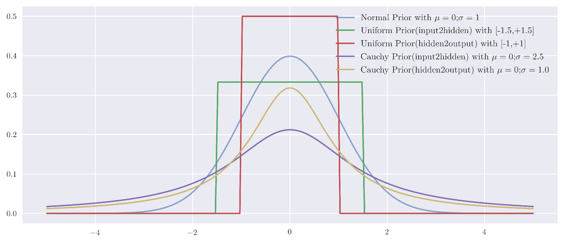
Argued in [30], differ than conventional implementation on Bayesian neural networks with the common used informative prior, the usage of weakly informative prior, i.e., a semi-flat prior, yielded superior predicative performance in single-label discrimination. Therefore, it is rational to extend this finding in multi-label learning. The formal definitions of informative and weakly informative priors are rendered below, and their corresponding probabilistic density curves are plotted in Figure 2. Their differentiated effects on a simple simulation is shown in Figure 3.

• Informative Prior

  – 

  Normal Prior

  $$\begin{array}{c}{\theta }_N\sim N(\mu ,{\sigma }^2)\end{array}$$

  (7)

  $$\begin{array}{c}p\left({\theta }_N\right)=\frac{1}{\sqrt{2\pi {\sigma }^2}}exp(-\frac{1}{2{\sigma }^2}{(\theta -\mu )}^2)\end{array}$$

  (8)

• Weakly Informative Prior

  – 

  Uniform Prior

  $$\begin{array}{c}{\theta }_U\sim U(\alpha ,\beta )\end{array}$$

  (9)

  $$\begin{array}{c}p\left({\theta }_U\right)=\frac{1}{\beta -\alpha }\end{array}$$

  (10)

  – 

  Cauchy Prior

  $$\begin{array}{c}{\theta }_C\sim Cauchy(\alpha ,\beta )\end{array}$$

  (11)

  $$\begin{array}{c}p\left({\theta }_C\right)=\frac{1}{\pi \beta (1+{(\frac{x-\alpha }{\beta })}^2)}\end{array}$$

  (12)

3.3. III. Model Uncertainty

In order to craft model uncertainty, we rely on the quantitative analysis of posterior predictive distribution under Bayesian neural networks. As the production of posterior predicative distribution entails the computation of the intractable parameter posterior, the common way is to approximate it via minimising the KL-divergence [23,31] ($KL\left(q\right|\left|p\right)={\sum }_{\theta }q\left(\theta \right)log\frac{q\left(\theta \right)}{p\left(x\right|\theta )}$) between approximated variational distribution, i.e., $q\left(\theta \right)$ and true posterior, i.e., $p\left(\theta \right|x)$, therefore solving for optimal posterior, i.e., $q^{\ast }\left(\theta \right)$, becomes:

$$q^{\ast }\left(\theta \right)=argmi{n}_{q\left(\theta \right)\in Q}KL\left(q\left(\theta \right)\left|\right|p\left(\theta \right|x)\right)$$

(13)

As we cannot compute the KL-divergence directly, the common approach is to resort on optimising an alternative objective, i.e., maximising the ELBO(evidence lower bound), derived as

$$ELBO\left(q^{\ast }\right)=\mathbb{E}\left[logp\left(x\right|\theta )\right]-KL(q\left(\theta \right)\left|\right|p\left(\theta \right))$$

(14)

Whereas $ELBO$ can be seen as a sum of the expected log likelihood of the data with the negative divergence between the variational variance and the model priors. Then it is customary to use the mean-field variational family to complete the specification of the above-mentioned optimisation. The mean-field variational family for each latent model parameter, i.e., $\theta$, can be defined:

$$q\left(\theta \right)={\Pi }_{j=1}^m{q}_j\left({\theta }_j\right)$$

(15)

Hence, finding the intractable posterior degrades to a coordinate ascent optimisation in obtaining the optimal ${\theta }^{\ast }$ in maximising $ELBO$ (cf. Algorithm 1 in [23] for detailed review). The learned optimal parameter posterior, e.g., $\left({\theta }_s\right|x)$ serves as a surrogate to be used in the parameter posterior in target BNN, i.e., $\left({\theta }_t\right|x)\left({\theta }_s\right|x)$. The model uncertainty, which is distilled from the source task, is now flowed to the target task.

3.4. IV. Prediction Related Uncertainty Indexes

With the flowed parameter posterior in the target task, i.e., $\left({\theta }_t\right|x)$, it is feasible to form the predictive posterior distribution for each upcoming novel observation, i.e., $x_{new}$, where,

$$p\left(x_{new}\right|x)={\int }_{{\theta }^{\ast }}p\left(x_{new}\right|{\theta }^{\ast })p\left(\theta \right|x)d\theta$$

(16)

Armed with this predictive posterior distribution, it allows the production of prediction related uncertainty indexes. As lengthy discussion in previous literature [20,32], one overwhelming claim insists that the probabilistic outputs can be produced by the soft-max function in (It is often placed in the final layer of neural networks to allow the real-valued prediction to be ’pushed’ in presenting the pseudo-probabilisitic output.) permitting the averaging over the repetitive forward propagations of new observation in either Bayesian neural network or non-Bayesian neural networks. This type of probabilistic output merely tells the most probable output given the input, not how uncertain is the prediction. For the comparative purpose, we refer this type of uncertainty index as soft-max uncertainty. The quantification of this soft-max uncertainty has been previously approximated via averaged T times of forward model(input) propagation [33], expressed in Equations (17) and (18):

$$\begin{array}{cc}\hfill Soft-Max& =\mathbb{E}(y\ast )\approx \frac{1}{T}\sum _{t=1}^T\left(\widehat{y\ast }\left(x_{new}\right)\right){|}_{p(\theta |x_{new})}\hfill \end{array}$$

(17)

$$\begin{array}{c}{=Class-Type|}_{Non-Bayesian}\hfill \end{array}$$

(18)

From Bayesian learning perspective, the above-mentioned softmax uncertainty reflects the belief of applying predictive mean in indexing the prediction uncertainty. Numerically, this type of uncertainty index captures the mere classification type in multiple-object discrimination, is equivalent with the class type probability in non-Bayesian neural networks. However, as the predictive mean does not capture the full picture of parameter posterior distribution, we draw our attention towards the predictive variance instead.

We argue that the yielded predictive variance reflects the degree of uncertainty that is associated with each prediction. As a result, based on the approximated weight posterior, i.e., $p\left(\theta \right|x)$, a better prediction related uncertainty index is expressed below in Equation (19):

$$Pure=Var[y\ast ]\approx Var\left[\sum _{t=1}^T{\int }_{\Theta }p\left(x_{new}\right)p\left(\theta \right|x)d\theta \right]$$

(19)

We denote this measure of prediction uncertainty index as pure uncertainty.

One step further, rather than the dichotomous uncertainty indexes, e.g., pure uncertainty and soft-max uncertainty, these two indexes can be fused together, which allows the uncertainty index to reflect both class-type probabilistic prediction and the model uncertainty associated with each prediction. In consistent with the previous naming tradition, this type of uncertainty index is marked as uncertainty plus. The production of this uncertainty plus shows that each class type probabilistic prediction should be proportionately adjusted according to its associated prediction uncertainty, expressed in Equation (20):

$$Uncert+\approx \frac{\frac{1}{T}{\sum }_{t=1}^T\left(\widehat{y\ast }\left(x_{new}\right)\right){|}_{p\left(\theta \right|x_{new})}}{Var\left[{\sum }_{t=1}^T{\int }_{\Theta }p\left(x_{new}\right)p\left(\theta \right|x)d\theta \right]}$$

(20)

For illustrative purposes, how each of three above mentioned uncertainty indexes, e.g., soft-max uncertainty, pure uncertainty, and uncertainty plus, influences on a simple binary classifier, is demonstrated in Figure 4.

4. Experiment

Relying on the transferred model uncertainty, the proposed Uncertainty Flow framework allows a learner to output multi-label predictions under single-label training curriculum. Empirical validation of our proposed framework contains two enquiries that need to be addressed. I.e., one is to investigate that whether or not our proposed Uncertainty Flow is superior to conventional multi-label learning algorithms in facilitating the zero-shot multi-label learning; whereas the other is to see which uncertainty index leads to the most significant performance elevation. Also, in order to investigate the role of suggested weakly informative priors, we additional specify our Uncertainty Flow into three types of priors. Hence, in total, there are three-level comparisons in our experiment, i.e., model comparison; prior comparison; and uncertainty comparison. The entire experiment is written in Python, using Theano [34], and Pymc3 [35] libraries. The partial code to produce this study is available from: https://github.com/LeonBai/Uncertainty-Flow.

4.1. Dataset

4.1.1. Training Dataset

We selected the first 1500 images from FER2013 [36] as our training dataset. The reason for intentional lowered size of training dataset is to enforce the similar model complexity between a source BNN and a target BNN. (cf. Figure 1). We leave the relaxation of such restriction to future research. FER2013 is a well researched public dataset, which is comprised of facial expression images for pictorial sentiment discrimination. Prior to our implementation, all images in this truncated version of FER2013 had gone through the standard preprocessing process, e.g., fixate the faces at centre, standardise the image size to 48 by 48 pixels in resolution, and all faces are properly registered. We then normalised the pixel values of input images. The original FER2013 images are labelled as one of seven emotion categories, e.g., angry, disgust, fear, happy, sad, surprise, and neutral.

4.1.2. Testing Dataset

To allow the evaluation of outputted multi-label predictions, it is imperative to rely on some existing benchmark annotations. Unfortunately, there is no current reliable multi-label annotations for FER2013 facial expressions. For this, we conducted a small-scale, i.e., 200 images, experiment on manual annotating the multi-label version of FER2013. The descriptive statistics of this annotated multi-label testing dataset is summarised in Appendix A, and the raw data can be found on https://github.com/LeonBai/Uncertainty-Flow. Preliminary statistic test revealed the high similarity between the original single-label and yielded multi-label annotations. I.e., treating the original single-label FER2013 annotations as ground truth, the overlaps between multi-label annotations and ground truth reached 75%, suggesting high similarity between two annotations. Indicated by a acceptable Fleiss-Kappa coefficient value [37], i.e., 0.25 (between −1 to 1, higher is more reliable)—the measurement of inter-rater reliability—the annotated multi-label version of FER2013 can be served as our testing dataset.

4.2. Models

To conduct an experiment that contains above-mentioned three-level comparisons, i.e., model comparison, prior comparison, uncertainty comparison, it demands explicit specification of all models in current experiment. In model comparison, four widely used multi-label learning algorithms, ranging from adaption algorithms, e.g., Multi-Label K-means Nearest Neighbour (MLkNN), Multi-label Neurofuzzy Classifier(ML-ARAM), to problem transformation algorithms, e.g., Binary Relevance (BR) and Label Powerset (LP), are included. In addition, two multi-label compatible neural networks. i.e., a multi-label feedforward Neural network (ML-FNN) and a multi-label convolutional neural network (ML-CNN), are also included in model comparison comparison.

In prior comparison and uncertainty comparison, depending on the prior type, i.e., informative or weakly informative, and different prediction related uncertainty indexes, e.g., soft-max uncertainty, pure uncertainty, uncertainty plus, the Uncertainty Flow generates 9 variants, denoting as BNN-normal-soft; BNN-normal-pure; BNN-normal-plus; BNN-uniform-soft; BNN-uniform-pure; BNN-uniform-plus; BNN-cauchy-soft; BNN-cauchy-pure; BNN-cauchy-plus. To further elevate the discriminative performance in multi-label prediction, we additional frame a convolutional neural network under Bayesian learning, producing Bayesian convolutional neural network within the proposed Uncertainty Flow framework, with its associated 9 variants, i.e., BCNN-normal-soft; BCNN-normal-pure; BCNN-normal-plus; BCNN-uniform-soft; BCNN-uniform-pure; BCNN-uniform-plus; BCNN-cauchy-soft; BCNN-cauchy-pure; BCNN-cauchy-plus. The configurations of above-mentioned models are summarised in Appendix B.

4.3. Evaluation Metrics

Different than the uniformed metric that used in single-label classification, i.e., classification accuracy, diversified evaluation metrics have been proposed. In line with the rouge classification from [11], we adhere the dichotomy classification of the evaluation metrics as bipartition and ranking based. For illustrative purposes, assuming a multi-label evaluation dataset is consist of input, i.e., $x_i$, and the set of true labels, i.e., $Y_i$, where $i=1,\dots ,m$ and $Y_i\subseteq L$, L is the set of all correct labels. Under this notation, the set of predicated labels are denoted as $Z_i$, where $i=1,\dots ,m$, while the rank predicted by learning method for a label $\lambda$ is denoted as $r_i\left(\lambda \right)$. The most relevant label, receives the highest rank (1), while the least relevant one, receives the lowest rank (q).

4.3.1. Bipartition Based

Delegated from the single-label metric, bipartition based metrics are proposed to capture the differences between actual and predicted sets of labels over all evaluation dataset. These differences can be computed in various means via either averaged over all samples or all label sets.

• Hamming loss

  $$Hamming-Loss=\frac{1}{m}\sum _{i=1}^{m_i}\frac{|Y_i△Z_i|}{M}$$

  (21)

  Where △ represents the symmetric difference of two sets, i.e., predicted and true label sets. Contrast with other over-strict measures of multi-label classification accuracy, i.e., low tolerance on partial label misclassification, e.g., $\frac{1}{m}{\sum }_{i_1}^{m}I|Y_i=Z_i|$, the hamming loss, which sums up to 1, offers a mild criteria for wider range of measurement application.
• Micro-Averaged F-Score & Average Precision
  Inherited from classic binary evaluation in information retrieval tasks, F-score and average precision, which both reflect their corresponded combinations of averaging over precision and recall, are two readily applicable metrics in multi-label learning. Among various averaging operations, e.g., macro, weighted, and micro, the preferred operation is micro-average as it offers each sample-class pair an equal contribution to the overall metric. Consider a binary evaluation measure $t_p,t_n,f_p,f_n$ that is computed via the number of true positives $t_p$, true negatives $t_n$, false positives $f_p$, false negatives $f_n$, the $nth$ threshold for precision and recall are $P_n$ and $R_n$, the interested micro-averaged F-score and average precision score(AP) are derived as following:

  $$\begin{array}{cc}\hfill P_n& =\frac{t_p}{t_p+f_p}\hfill \end{array}$$

  (22)

  $$\begin{array}{cc}\hfill R_n& =\frac{t_p}{t_p+f_n}\hfill \end{array}$$

  (23)

  $$\begin{array}{cc}\hfill MicroAveraged\left(F_{\beta }\right)& =(1+{\beta }^2\frac{P_n\times R_n}{{\beta }^2{P}_n+R_n})\hfill \end{array}$$

  (24)

  $$\begin{array}{cc}\hfill AveragePreision\left(AP\right)& =\sum _n(R_n-R_{n-1})P_n\hfill \end{array}$$

  (25)

4.3.2. Ranking Based

• Converge
  To measure the needed distance to cover all true label sets, i.e., $Y_i$ in the predicted label sets, we resort on the converge error metric. It can be defined as following:

  $$\begin{array}{c}Coverage-Error=\frac{1}{m}\sum _{i=1}^{m}ma{x}_{\lambda \in Y_i}{r}_i\left(\lambda \right)-1\end{array}$$

  (26)
• Ranking Loss
  The ranking loss targets at the incorrect ordering of the predicted label sets. Presume $\overline{Y_i}$ is expressed as the complementary set of $Y_i$, its computation can be defined as following:

  $$R-Loss=\frac{1}{m}\sum _{i=1}^m\frac{1}{|Y_i\left|\right|{\overline{Y}}_i|}\{({\lambda }_a,{\lambda }_b):r_i\left({\lambda }_a\right)>r_i\left({\lambda }_b\right),({\lambda }_a,{\lambda }_b)\in Y_i\times \overline{Y_i}\}$$

  (27)

4.4. Results & Discussion

The overall result of our conducted large-scale comparative experiment is chiefly presented in

Table 1. Model Comparison in Various Multi-label Evaluation Metrics.

Candidate Models	Hamming-Loss	Converge-Loss	Ranking-Loss	F-Score	Average Precision	Source
Conventional Multi-Label Models
MLkNN	0.286	7.000	0.950	0.090	0.346	[14]
ML-ARAM	0.374	6.670	0.801	0.264	0.369	[13]
Binary Relevance	0.275	7.00	1.000	0.263	0.340	[38]
Label Powerset	0.328	6.940	0.837	0.215	0.370	[39]
Multi-Label Compatible Neural Networks
ML-FNN	0.402	6.700	0.761	0.282	0.376	[40]
ML-CNN	0.387	6.600	0.733	0.3108	0.384	[41]
Uncertainty Flow - Bayesian Neural Networks
BNN-normal-soft	0.404	6.500	0.75	0.279	0.360	This research
BNN-normal-pure	0.382	6.500	0.723	0.318	0.389	This research
BNN-normal-plus	0.402	6.673	0.759	0.282	0.525	This research
BNN-uniform-soft	0.414	6.750	0.7816	0.302	0.353	This research
BNN-uniform-pure	0.385	6.450	0.723	0.330	0.389	This research
BNN-uniform-plus	0.404	6.450	0.765	0.310	0.530	This research
BNN-cauchy-soft	0.400	6.7	0.759	0.285	0.378	This research
BNN-cauchy-pure	0.382	6.525	0.727	0.312	0.402	This research
BNN-cauchy-plus	0.401	6.250	0.741	0.290	0.527	This research
Uncertainty Flow - Bayesian Convolutional Neural Networks
BCNN-normal-soft	0.421	6.750	0.791	0.250	0.385	This research
BCNN-normal-pure	0.384	6.700	0.737	0.319	0.449	This research
BCNN-normal-plus	0.400	6.675	0.751	0.288	0.561	This research
BCNN-uniform-soft	0.403	6.675	0.762	0.282	0.421	This research
BCNN-uniform-pure	0.404	6.800	0.769	0.279	0.311	This research
BCNN-uniform-plus	0.387	6.725	0.736	0.310	0.527	This research
BCNN-cauchy-soft	0.401	6.675	0.760	0.285	0.416	This research
BCNN-cauchy-pure	0. 396	6.800	0.753	0.322	0.390	This research
BCNN-cauchy-plus	0.401	6.75	0.758	0.285	0.576	This research

. For illustrative purposes, we grouped the results to highlight the comparison among different models. As we used various of evaluation metrics to assess the performance of corresponding models, it is difficulty to obtain a clear judgement that is based on single metric. I.e., when we pitted our approach, i.e., Uncertainty Flow against the MLkNN approach in conventional multi-label models, our approach, including all nine variations, is inferior to the MLkNN approach on the metric of Hamming-Loss. However, when we accessed the model according to its performance on Average Precision, our approach largely outperformed the MLkNN approach. Moreover, as we incorporated nine variations in Uncertainty Flow, the in-depth analyses of the prior types and uncertainty indexes are demanded. We then divided our discussion of the overall result into three parts, e.g., the results on model comparison, the results on prior comparison, and the results on uncertainty comparison.

4.4.1. Model Comparison

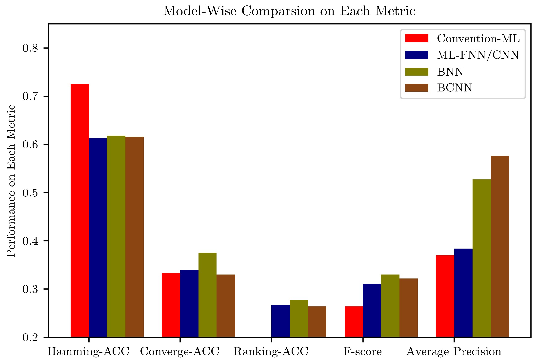
Ruling out the factors of prior types and prediction related uncertainty indexes, the empirical comparison between Uncertainty Flow framework and the alternatives demonstrated mixed results, illustrated in Figure 5.

Previous findings from [11] and [6] stated that it is practical difficult to observe a single model or algorithm, which is competitive enough to beat others in every multi-label evaluation metric. Hence, it is imperative to investigate each loss metric independently. Focusing on Hamming-Loss (Hamming-ACC = 1 − Hamming loss), interestingly, the conventional multi-label learning models are particular good in minimising this type of loss. However, indicated in Converge-Loss and Ranking-Loss, both Uncertainty Flow and multi-label compatible neural networks, e.g., ML-FNN and ML-CNN are superior than the conventional multi-label learning alternatives.

Under two precision related metrics, e.g., F-score and average precision, with the help from a weakly informative prior, e.g., uniform or Cauchy prior, and an advanced prediction related uncertainty indexes, e.g., pure uncertainty, or uncertainty plus, both BNN and BCNN, exhibited clear performance advantage over their alternatives, e.g., ML-FNN, ML-CNN and conventional multi-label models. Especially on the metric of average Precision, the nontrivial performance enhancement, i.e., over 20% accuracy increase, demonstrated the superior discriminability that tags to our proposed Uncertainty Flow. Moreover, comparing the performance between BNN and BCNN, the convolutional architecture, e.g., BCNN, should be credited for overall performance improvement.

4.4.2. Prior Comparison

To verify the most applicable prior in our proposed Uncertainty Flow, the prior comparison among three candidate priors is worthy to be fully investigated. Shown in Figure 6b, despite some similarities in shapes, it is clear that each prior has its unique effect in shaping the corresponded posterior distribution of the weights. In specific, the effect of uniform prior on posterior weight is seen as the restriction on the approximated posterior weights, i.e., the posterior weights have to be higher than a fixed value, e.g., 1 in our implementation. This restriction effect may lower the discriminability of the uniform prior imposed model, shown in Figure 7. Interestingly, the posterior distribution of weights from imposed normal and Cauchy priors respectively rendered nearly identical distribution shape, shown in Figure 6a,c. The minute difference between these two is the enlarged variance for Cauchy prior induced posterior distribution of weights. Despite seemingly trivial, this difference in variance lead to the discrepancy in discriminative performance, shown in Figure 7. Overall, based on final induced discriminability, a Cauchy prior is considered as the most applicable prior in our proposed Uncertainty Flow.

The performance enhancement that can be reflected by above-mentioned ’clustered’ effect in weight posterior was observed in examination of the discriminability of three implemented prior. Plotted in Figure 7, focusing on the average precision evaluation metric, regardless of the variations in Bayesian neural networks, i.e., BNN or BCNN, the employment of Cauchy prior—as one kind of weakly informative prior–leaded competitive multi-label affective classification. However, as another implemented weakly informative prior, uniform prior was inferior to the used informative prior, e.g., normal prior. This observed attenuation in discriminability from uniform prior may due to the its above-mentioned spike-and-slab effect on weight posterior that requires extra training epochs to stabilise the pre-to-posterior inference.

4.4.3. Uncertainty Comparison

Undoubtedly, the most pronounced performance improvement is pertaining to the inclusion of advanced prediction related uncertainty indexes, e.g., pure uncertainty and uncertainty plus. To recall the foregoing definition of prediction related uncertainty indexes, the soft-max uncertainty is a mere indication of multi-class prediction type, which is equivalent with the predictions in non-Bayesian alternatives. The pure uncertainty, i.e., on the contrary—depends heavily on weight posterior—can be produced exclusively in our proposed Uncertainty Flow framework. Reflected in Figure 8, when the feedforward architecture was adopted, soft-max uncertainty is inferior to pure uncertainty in producing multi-label prediction. Interestingly, when the convolutional architecture was chosen, it uncovered a different story, i.e., the discriminability from pure uncertainty became inferior to soft-max uncertainty.

Not surprisingly, the combination of soft-max uncertainty and pure uncertainty, i.e., the craft of uncertainty plus, allows a set of multi-label predictions to be tuned based on its uncertainty value. Shown in Figure 8, it is clear that the crafted predictions that are benefited from Uncertainty plus are superior to other two uncertainty indexes. I.e., its introduced improvement in average precision is over 20% compare to other two indexes. Combining the most applicable weakly informative prior and the advanced uncertainty indexe together, the two most efficient variants in feedforward and convolutional architectures are BNN-cauchy-plus and BCNN-cauchy-plus, respectively. We leave sensitivity analysis of our proposed advanced uncertainty indexes to future research.

5. Conclusions

Over reliance on single-label affective learning hinders the fruition of the automatic affective analysis. To free from this restriction, we resort on multi-label affective learning. However, current multi-learning algorithms are not scalable enough due to the scarcity of multi-label training samples. To tackle this issue, we propose a inductive transfer learning based framework, i.e., Uncertainty Flow. Under this pioneer framework, we argue that the model uncertainty can be distilled from a source single-label recognition task. The distilled knowledge is then fed to a to-be-learned multi-label affective recognition task. For predictions, three types of uncertainty indexes, i.e., soft-max uncertainty, pure uncertainty, and uncertainty plus, are further proposed. For empirical validation, the authors conducted a large-scale comparative experiment on the manual annotated multi-label FER2013 dataset across three levels of comparisons, i.e., model comparison, prior comparison, and uncertainty comparison. The observed performance superiority in Uncertainty Flow unequivocally renders the feasibility of applying this framework in zero-shot multi label affective learning.

However, even under the permitted computational resources, to run a full Bayesian posterior remains as a daunting task. How to speed up the posterior inference is an open research question. In terms of future researches, there are two streams of researches that are worthy to be further explored. One focuses on improving the discriminability of our novel proposed Uncertainty Flow framework. This entails the revision on the mainstream mean field based variational inference [23]. The other is to extend the current inductive transfer based framework to the transductive transfer domain [7], where has already been demonstrated in vivo [42].

References

- Hassin, R.R.; Aviezer, H.; Bentin, S. Inherently Ambiguous: Facial Expressions of Emotions, in Context. Emot. Rev. 2013, 5, 60–65. [Google Scholar] [CrossRef]
- Kumar, B.V. Face expression recognition and analysis: The state of the art. arXiv, 2009; arXiv:1203.6722. [Google Scholar]
- Sariyanidi, E.; Gunes, H.; Cavallaro, A. Automatic Analysis of Facial Affect: A Survey of Registration, Representation, and Recognition. IEEE Trans. Pattern Anal. Mach. Intell. 2015, 37, 1113–1133. [Google Scholar] [CrossRef] [PubMed]
- Barsoum, E.; Zhang, C.; Ferrer, C.C.; Zhang, Z. Training Deep Networks for Facial Expression Recognition with Crowd-Sourced Label Distribution. In Proceedings of the 18th ACM International Conference on Multimodal Interaction, Tokyo, Japan, 12–16 November 2016. [Google Scholar]
- Bai, W.; Luo, W. Hard Label Relaxation in Biased Pictorial Sentiment Discrimination. In Proceedings of the Natural Language Processing and Knowledge Engineering, Chengdu, China, 7–10 December 2017. [Google Scholar]
- Madjarov, G.; Kocev, D.; Gjorgjevikj, D.; Džeroski, S. An extensive experimental comparison of methods for multi-label learning. Pattern Recognit. 2012, 45, 3084–3104. [Google Scholar] [CrossRef]
- Pan, S.J.; Yang, Q. A survey on transfer learning. IEEE Trans. Knowl. Data Eng. 2010, 22, 1345–1359. [Google Scholar] [CrossRef]
- Neal, R.M. Bayesian Learning for Neural Networks; Springer Science & Business Media: Berlin, Germany, 2012; Volume 118. [Google Scholar]
- Perikos, I.; Ziakopoulos, E.; Hatzilygeroudis, I. Recognizing emotions from facial expressions using neural network. In IFIP International Conference on Artificial Intelligence Applications and Innovations; Springer: Berlin, Germany, 2014; pp. 236–245. [Google Scholar]
- Filko, D.; Martinovic, G. Emotion Recognition System by a Neural Network Based Facial Expression Analysis. Automatika 2013, 54, 263–272. [Google Scholar] [CrossRef]
- Tsoumakas, G.; Katakis, I.; Vlahavas, I. Mining multi-label data. In Data Mining and Knowledge Discovery Handbook; Springer: Berlin, Germany, 2009; pp. 667–685. [Google Scholar]
- Luaces, O.; Díez, J.; Barranquero, J.; del Coz, J.J.; Bahamonde, A. Binary relevance efficacy for multilabel classification. Prog. Artif. Intell. 2012, 1, 303–313. [Google Scholar] [CrossRef]
- Benites, F.; Sapozhnikova, E. HARAM: A Hierarchical ARAM neural network for large-scale text classification. In Proceedings of the 2015 IEEE International Conference on the Data Mining Workshop (ICDMW), Atlantic City, NJ, USA, 14–17 November 2015; pp. 847–854. [Google Scholar]
- Zhang, M.L.; Zhou, Z.H. ML-KNN: A lazy learning approach to multi-label learning. Pattern Recognit. 2007, 40, 2038–2048. [Google Scholar] [CrossRef]
- Zhang, M.L.; Zhou, Z.H. Multilabel neural networks with applications to functional genomics and text categorization. IEEE Trans. Knowl. Data Eng. 2006, 18, 1338–1351. [Google Scholar] [CrossRef]
- Mower, E.; Mataric, M.J.; Narayanan, S. A Framework for Automatic Human Emotion Classification Using Emotion Profiles. IEEE Trans. Audio Speech Lang. Process. 2011, 19, 1057–1070. [Google Scholar] [CrossRef]
- Mower, E.; Metallinou, A.; Lee, C.C.; Kazemzadeh, A.; Busso, C.; Lee, S.; Narayanan, S. Interpreting ambiguous emotional expressions. In Proceedings of the 3rd International Conference on Affective Computing and Intelligent Interaction and Workshops, Amsterdam, The Netherlands, 10–12 September 2009; pp. 1–8. [Google Scholar]
- Zhao, K.; Zhang, H.; Ma, Z.; Song, Y.Z.; Guo, J. Multi-label learning with prior knowledge for facial expression analysis. Neurocomputing 2015, 157, 280–289. [Google Scholar] [CrossRef]
- Ghahramani, Z. Probabilistic machine learning and artificial intelligence. Nature 2015, 521, 452–459. [Google Scholar] [CrossRef] [PubMed]
- Denker, J.S.; Lecun, Y. Transforming neural-net output levels to probability distributions. In Proceedings of the Advances in Neural Information Processing Systems, Denver, CO, USA, 2–5 December 1991; pp. 853–859. [Google Scholar]
- Tishby, N.; Levin, E.; Solla, S.A. Consistent inference of probabilities in layered networks: Predictions and generalization. Int. Jt. Conf. Neural Netw. 1989, 2, 403–409. [Google Scholar]
- Gal, Y.; Ghahramani, Z. Bayesian Convolutional Neural Networks with Bernoulli Approximate Variational Inference. arXiv, 2015; arXiv:1506.02158. [Google Scholar]
- Blei, D.M.; Kucukelbir, A.; McAuliffe, J.D. Variational Inference: A Review for Statisticians. J. Am. Stat. Assoc. 2017, 112, 859–877. [Google Scholar] [CrossRef]
- Williams, P.M. Bayesian Regularization and Pruning Using a Laplace Prior. Neural Comput. 1995, 7, 117–143. [Google Scholar]
- Gülçehre, C.; Bengio, Y. Knowledge matters: Importance of prior information for optimization. J. Mach. Learn. Res. 2016, 17, 1–32. [Google Scholar]
- Jeffreys, H. An invariant form for the prior probability in estimation problems. Proc. R. Soc. Lond. A 1946, 186, 453–461. [Google Scholar] [CrossRef]
- Bernardo, J.M. Reference posterior distributions for Bayesian inference. J. R. Stat. Soc. Ser. B 1979, 41, 113–147. [Google Scholar]
- Gelman, A. Prior distributions for variance parameters in hierarchical models (comment on article by Browne and Draper). Bayesian Anal. 2006, 1, 515–534. [Google Scholar] [CrossRef]
- Gelman, A.; Jakulin, A.; Pittau, M.G.; Su, Y.S. A weakly informative default prior distribution for logistic and other regression models. Ann. Appl. Stat. 2008, 2, 1360–1383. [Google Scholar] [CrossRef]
- Bai, W.; Quan, C. Harness the Model Uncertainty via Hierarchical Weakly Informative Priors in Bayesian Neural Network. Int. Rob. Auto. J. 2017, 3. [Google Scholar] [CrossRef]
- Jordan, M.I.; Ghahramani, Z.; Jaakkola, T.S.; Saul, L.K. An introduction to variational methods for graphical models. Mach. Learn. 1999, 37, 183–233. [Google Scholar] [CrossRef]
- Lee, W.T.; Tenorio, M.F. On Optimal Adaptive Classifier Design Criterion: How Many Hidden Units are Necessary for an Optimal Neural Network Classifier? Purdue University, School of Electrical Engineering: West Lafayette, IN, USA, 1991. [Google Scholar]
- Srivastava, P.; Hopwood, N. A practical iterative framework for qualitative data analysis. Int. J. Qual. Methods 2009, 8, 76–84. [Google Scholar] [CrossRef]
- Bergstra, J.; Breuleux, O.; Bastien, F.; Lamblin, P.; Pascanu, R.; Desjardins, G.; Turian, J.; Warde-Farley, D.; Bengio, Y. Theano: A CPU and GPU math compiler in Python. In Proceedings of the 9th Python in Science Conference, Austin, TX, USA, 28 June–3 July 2010; pp. 1–7. [Google Scholar]
- Salvatier, J.; Wiecki, T.V.; Fonnesbeck, C. Probabilistic programming in Python using PyMC3. PeerJ Comput. Sci. 2016, 2, e55. [Google Scholar] [CrossRef]
- Goodfellow, I.J.; Erhan, D.; Carrier, P.L.; Courville, A.; Mirza, M.; Hamner, B.; Cukierski, W.; Tang, Y.; Thaler, D.; Lee, D.H. Challenges in representation learning: A report on three machine learning contests. In International Conference on Neural Information Processing; Springer: Berlin, Germany, 2013; pp. 117–124. [Google Scholar]
- Fleiss, J.L.; Cohen, J. The equivalence of weighted kappa and the intraclass correlation coefficient as measures of reliability. Educ. Psychol. Meas. 1973, 33, 613–619. [Google Scholar] [CrossRef]
- Read, J.; Pfahringer, B.; Holmes, G.; Frank, E. Classifier chains for multi-label classification. In Machine Learning and Knowledge Discovery in Databases; Springer: Berlin, Germany, 2009; pp. 254–269. [Google Scholar]
- Tsoumakas, G.; Vlahavas, I. Random k-labelsets: An ensemble method for multilabel classification. In Machine learning: ECML 2007; Springer: Berlin, Germany, 2007; pp. 406–417. [Google Scholar]
- Zhang, M.L. ML-RBF: RBF neural networks for multi-label learning. Neural Process. Lett. 2009, 29, 61–74. [Google Scholar] [CrossRef]
- Wei, Y.; Xia, W.; Lin, M.; Huang, J.; Ni, B.; Dong, J.; Zhao, Y.; Yan, S. HCP: A flexible CNN framework for multi-label image classification. IEEE Trans. Pattern Anal. Mach. Intell. 2016, 38, 1901–1907. [Google Scholar] [CrossRef] [PubMed]
- Nook, E.C.; Lindquist, K.A.; Zaki, J. A new look at emotion perception: Concepts speed and shape facial emotion recognition. Emotion 2015, 15, 569–578. [Google Scholar] [CrossRef] [PubMed]
Figure 1.
Uncertainty Flow Framework. The graphic model explanation of our proposed Uncertainty Flow framework shows four essential elements. I.e., the dual Bayesian neural networks in I, e.g., a source and a target BNN(separate by different colours in Figure 1); the weakly informative prior in II; the quantification of model uncertainty in III; and three proposed uncertainty indexes in perfecting the final multi-label categorisation in IV.
Figure 2.
The Probabilistic Density Curves of Normal, Uniform, and Cauchy Priors. This graph demonstrates the probabilistic density curve for each of the prior applied in this research, i.e., Normal, Uniform and Cauchy priors. Here, the further specification of input-to-hidden, hidden-to-hidden priors are defined as the hierarchical shrinkage in variance of the corresponding priors.
Figure 3.
Effects of Different Priors on Posterior in a Simulated Binary Classification. Note, here, the simulated posterior inferences were based on a simple three layer Bayesian neural network with five units in the hidden layer on a binary classification problem. Left panel of Figure 3 reflects how prior, i.e., denoted as red and blue dotted lines, transformed to the weight posterior, i.e., identified as green and light blue lines. The right panel of Figure 3 demonstrates the sampling value of yielded weight posterior, based on 500 posterior samples. Reflected by the separateness of yielded weight posterior, it is clear that Cauchy prior achieved the most discriminability compare to other two priors, e.g., Normal and Uniform priors.
Figure 4.
Comparison of Three Prediction Related Uncertainty Indexes on a Binary Classifier. In this figure, three different means of crafting uncertainty boundary for obtaining classification prediction on a simple binary classification problem, i.e., two classes are separated by blue and red, is delineated.
Figure 5.
Model Wise Comparison on Multi-learning Metrics. Note here, for illustrative purposes, we used Hamming-ACC, Converge-ACC and Ranking-ACC instead of original loss based metrics. Rather than the averaging over the models in each category, e.g., Conventional-ML, we picked the most representative model in each category for different metric.
Figure 6.
Different Priors on Posterior Weights Under Uncertainty Flow. Note here, the notation means posterior weights in first hidden layer in our implemented BNN or BCNN.
Figure 7.
Prior Induced Discriminability Differences in Uncertainty Flow. Note here, we rule out the impacts of uncertainty indexes via averaging the performance of models with same implemented prior. Average precision is chosen as other metrics failed to render clear discriminability comparison.
Figure 8.
Discriminative Performance Across Different Prediction Related Uncertainty Indexes. Note here, the effects of priors were marginalised via prior-wise averaging.