Noncontact Surface Roughness Estimation Using 2D Complex Wavelet Enhanced ResNet for Intelligent Evaluation of Milled Metal Surface Quality

 ,
,
Abstract
:1. Introduction
- (1)
- A texture skew correction method, based on the combination of an improved Sobel operator and Hough transform, is proposed for the surface texture direction adjustment. The results show that the proposed method is able to correct texture skew.
- (2)
- The paper proposes an intelligent surface roughness evaluation method based on machine-vision-enhanced artificial intelligence technology for 2D images. After 2D-DTCWT filtering of adjusted images, ResNet is employed for the surface texture pattern recognition. Owing to the engagement of ResNet in artificial feature learning, the model does not rely on prior knowledge.
- (3)
- Surface roughness estimation using the proposed method was performed on the images of milled metal surfaces made from the material spheroidal graphite cast iron 500-7. The high estimation accuracy of surface roughness revealed by the experimental results shows that the proposed method has good generalization ability.
2. Image Pre-Processing
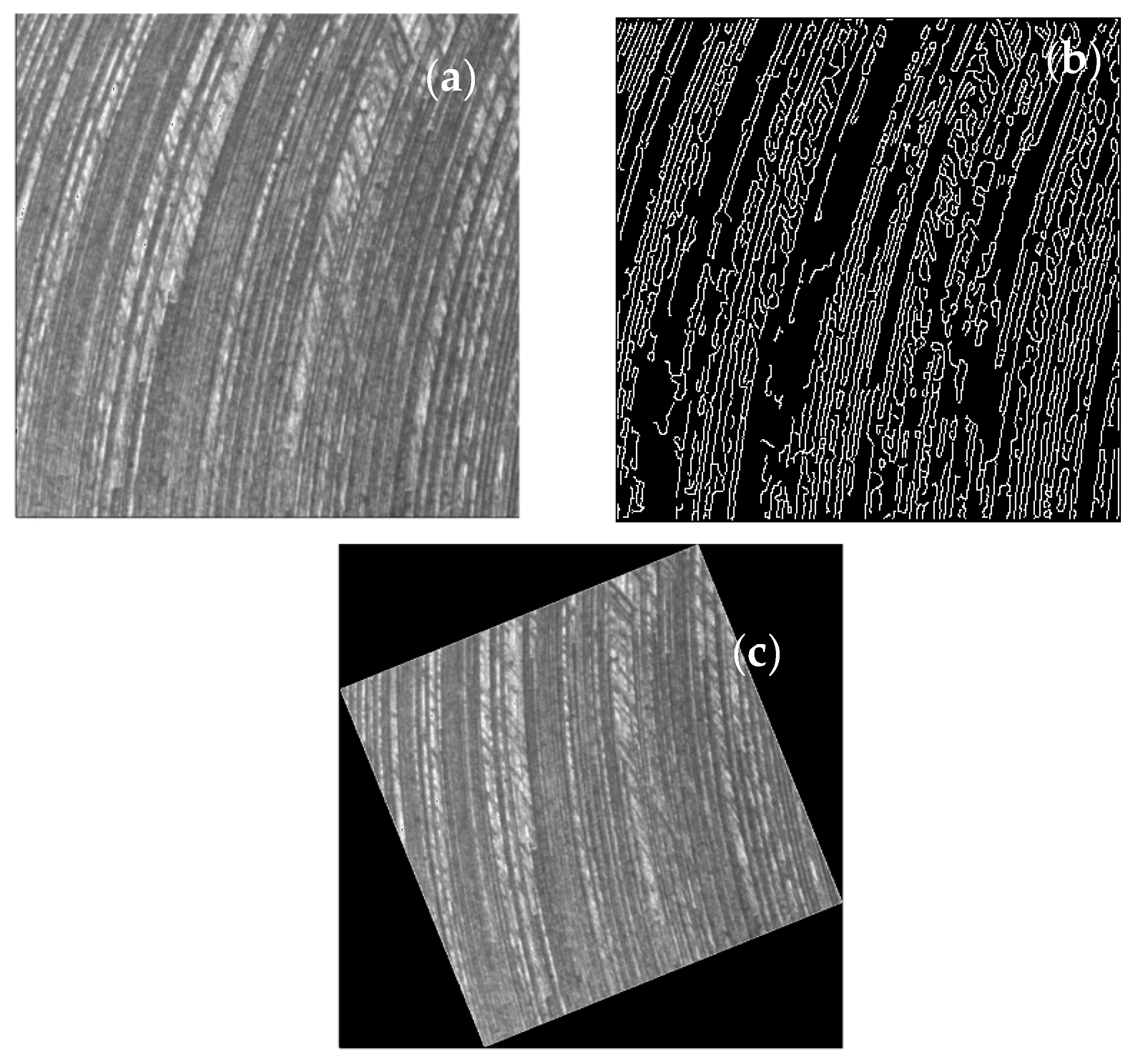
2.1. Improved Texture Skew Correction
2.1.1. Improved Sobel Operator
- (1)
- Initialization such that Max = v{0}, t = 1.
- (2)
- If v{t} > Max, set Max = v{t}
- (3)
- If t < 8, then t = t + 1 and go to (2). If not, go to Step 3.
2.1.2. Hough Transform
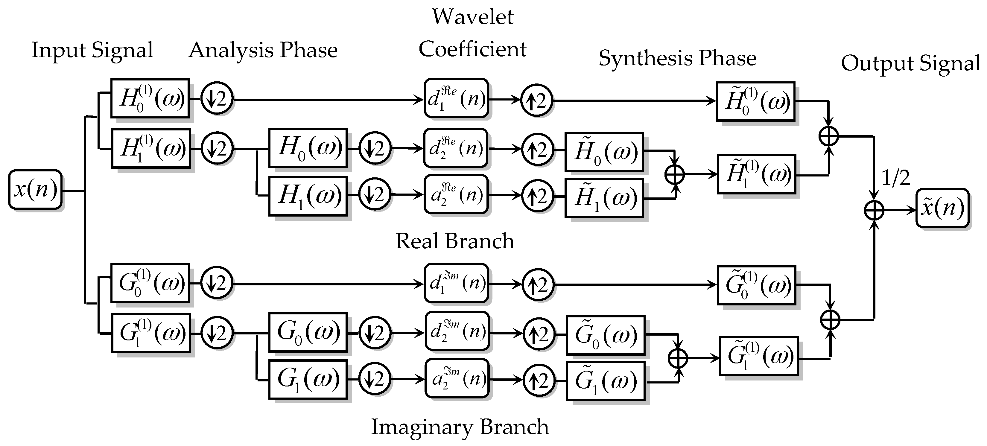
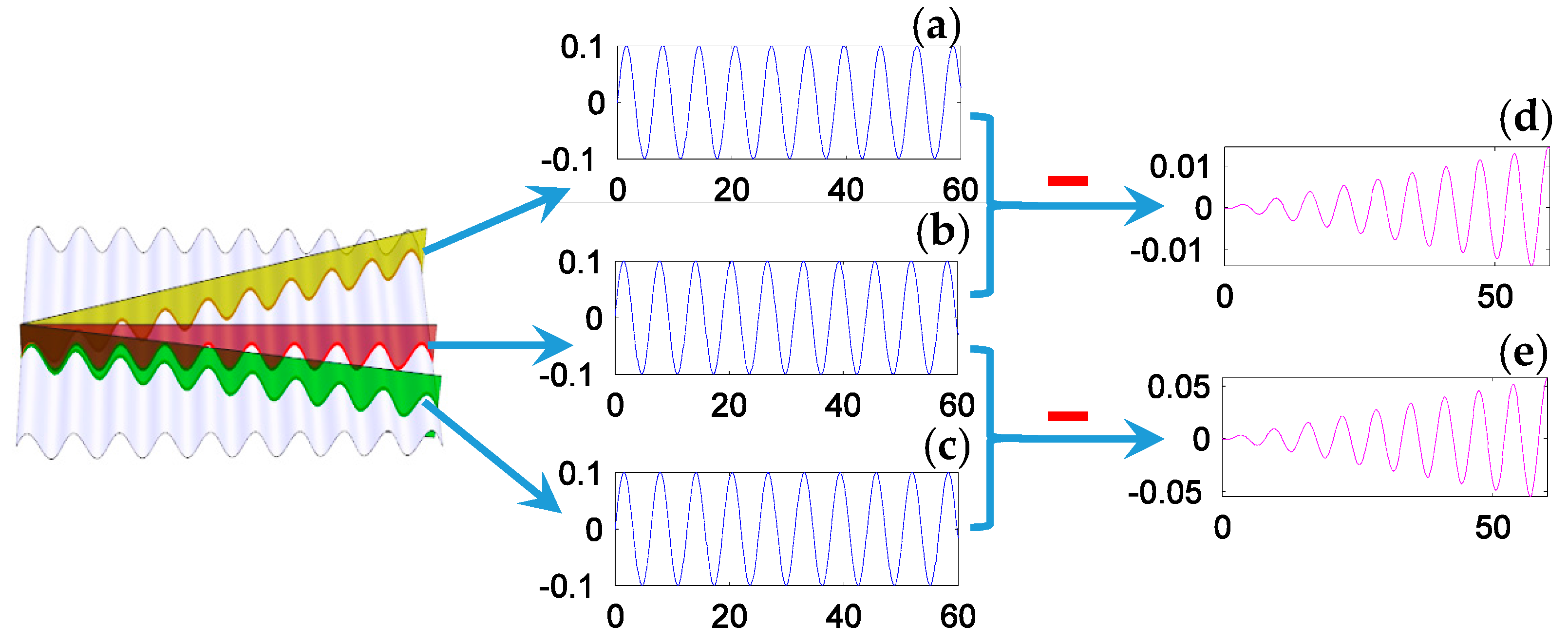
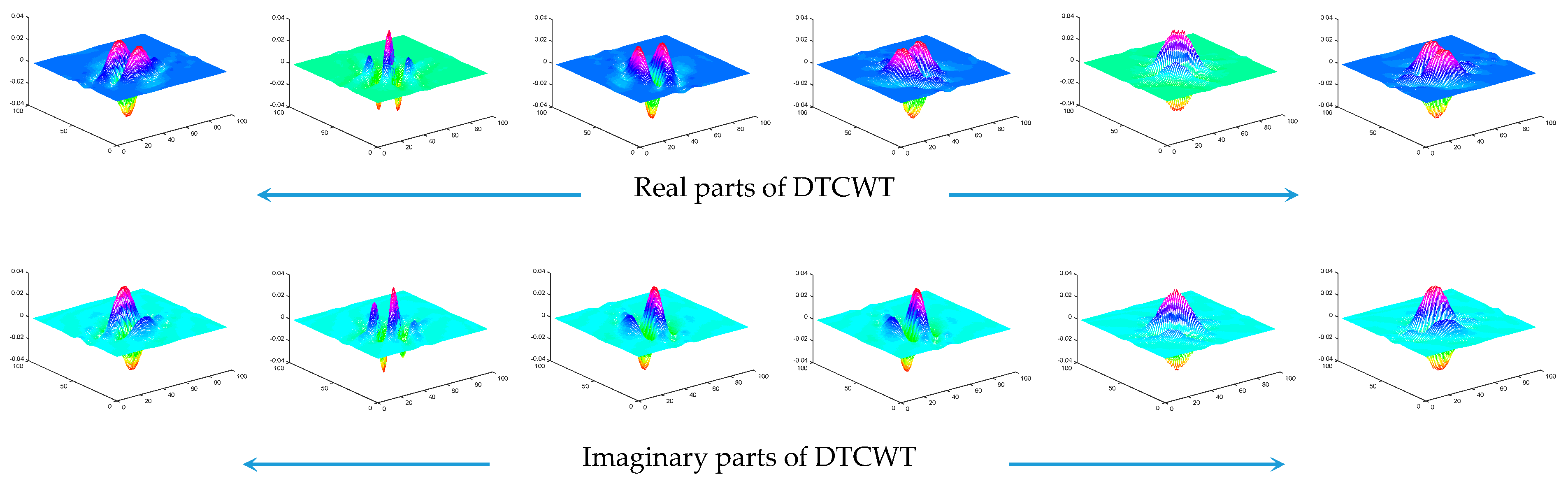
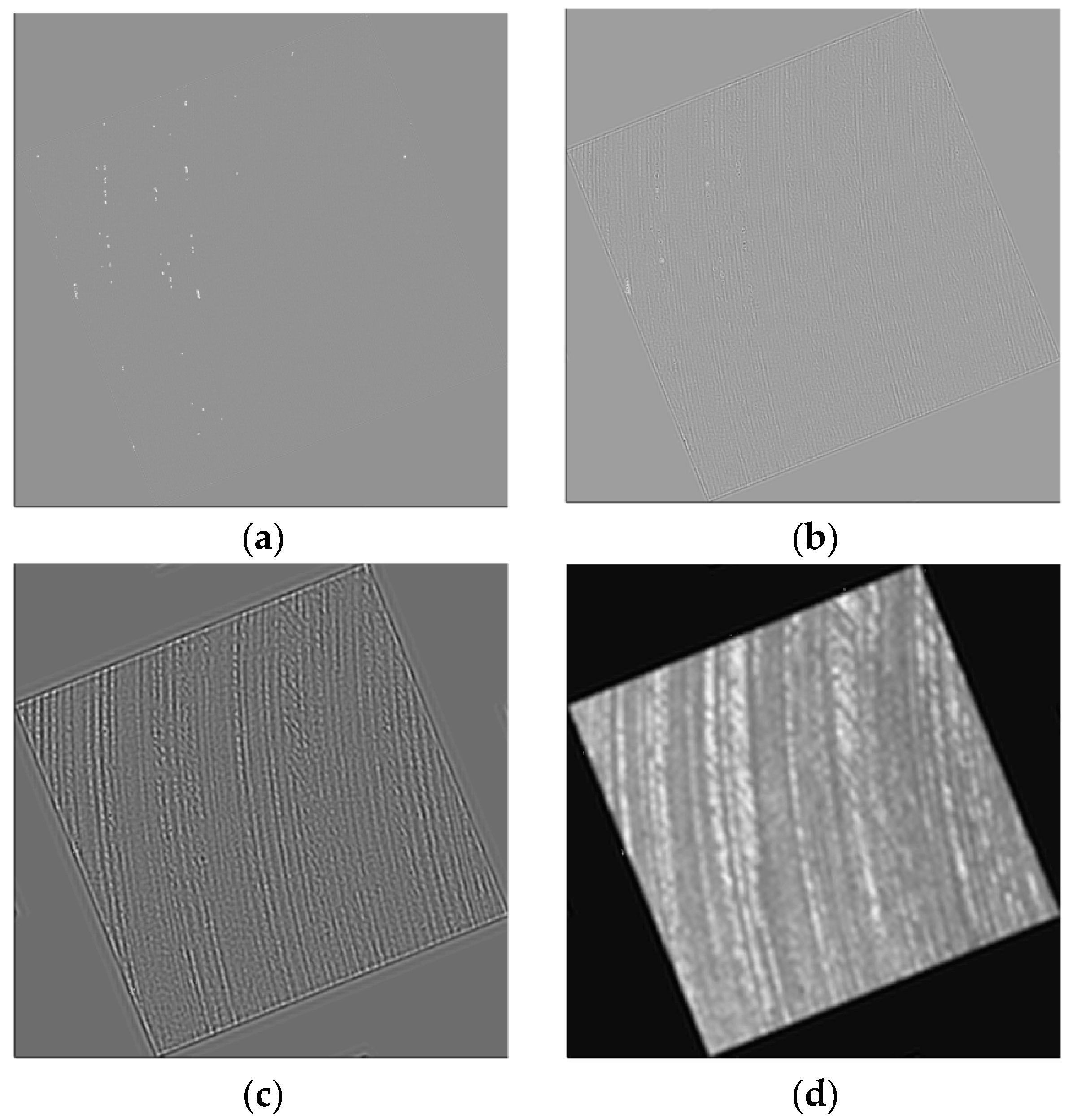
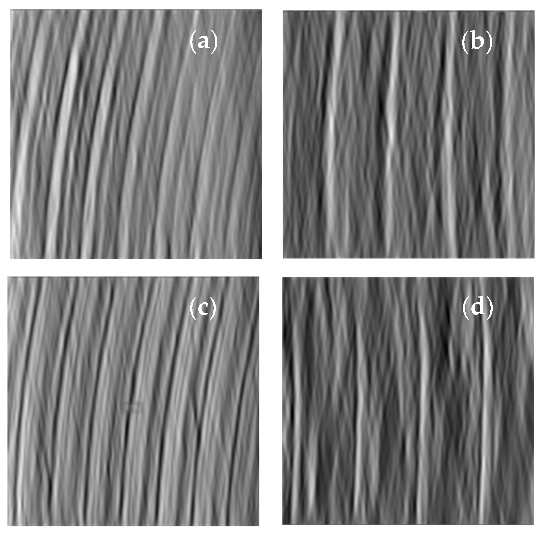
2.2. Two-Dimensional Dual Tree Complex Wavelet Transform (2D-DTCWT)
2.2.1. Framework of DTCWT
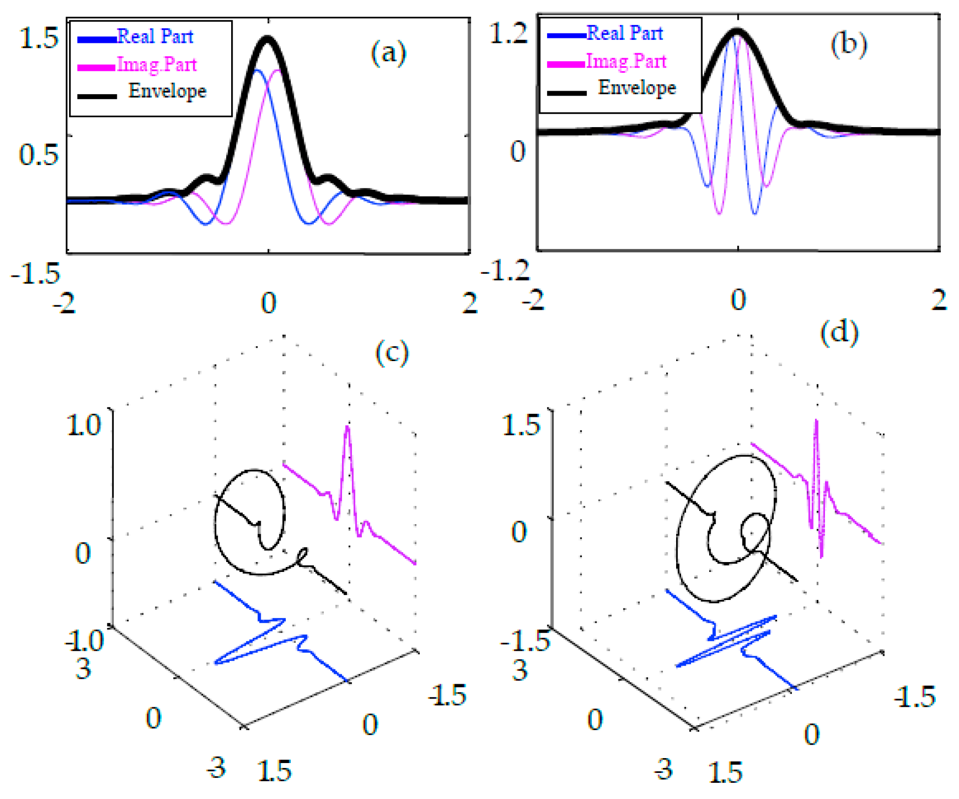
2.2.2. Nearly Analytic Complex Wavelet Basis
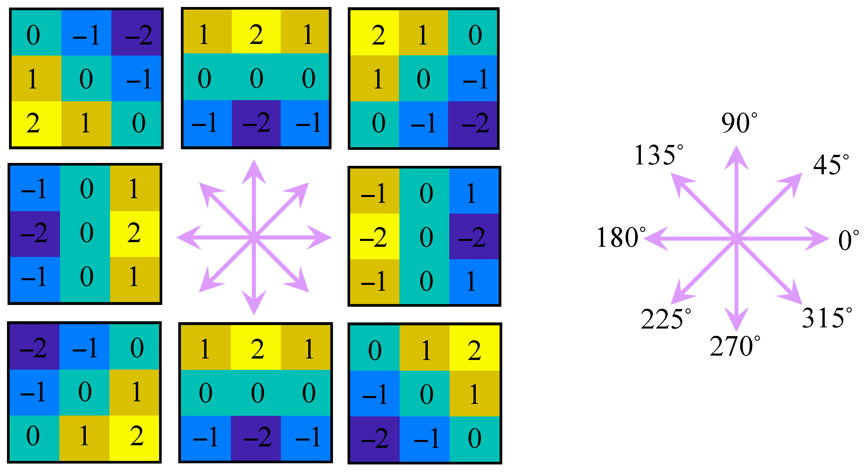
2.2.3. Directional Filtering Atoms of 2D-DTCWT
3. Intelligent Learning Method Based on ResNet
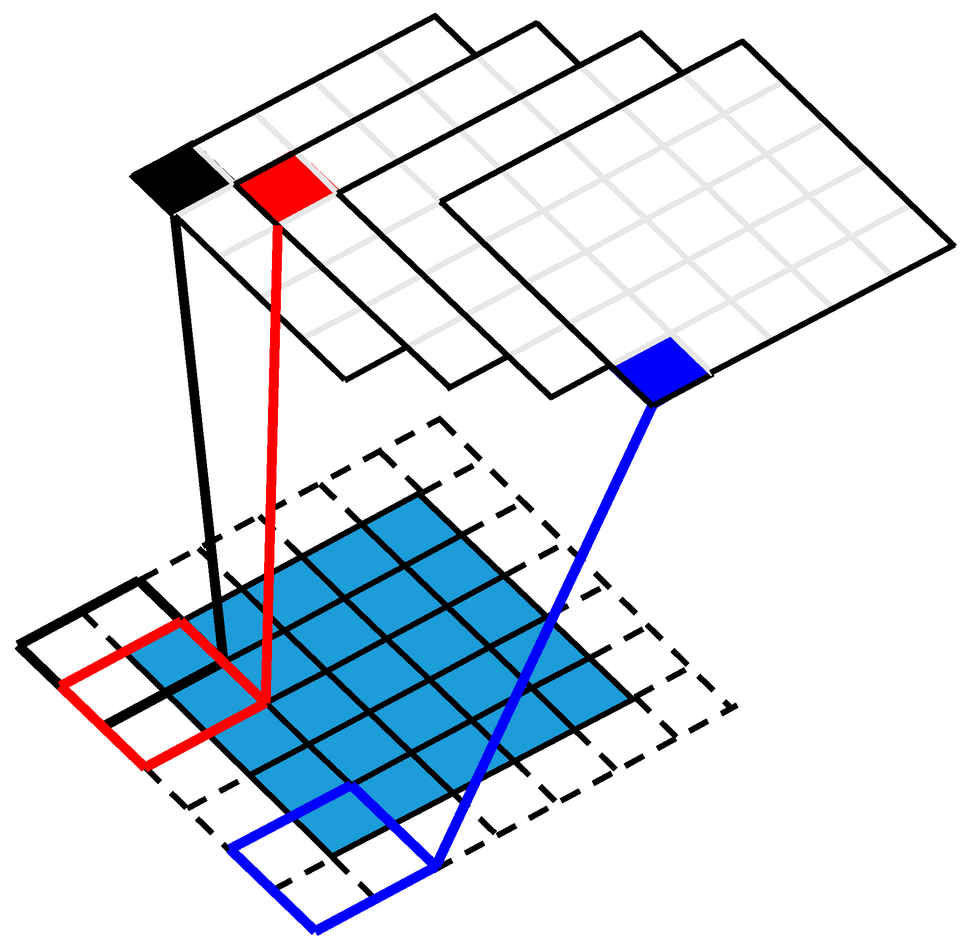
3.1. Convolutional Layer
3.2. Polling Layer
3.3. Output Layer
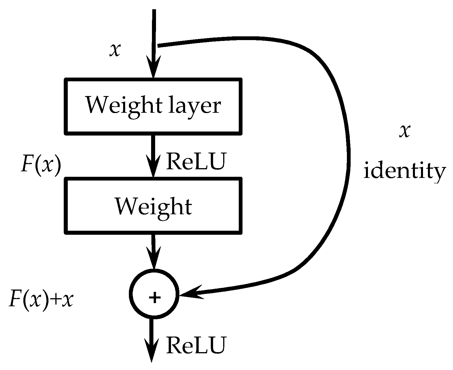
3.4. Residual Block
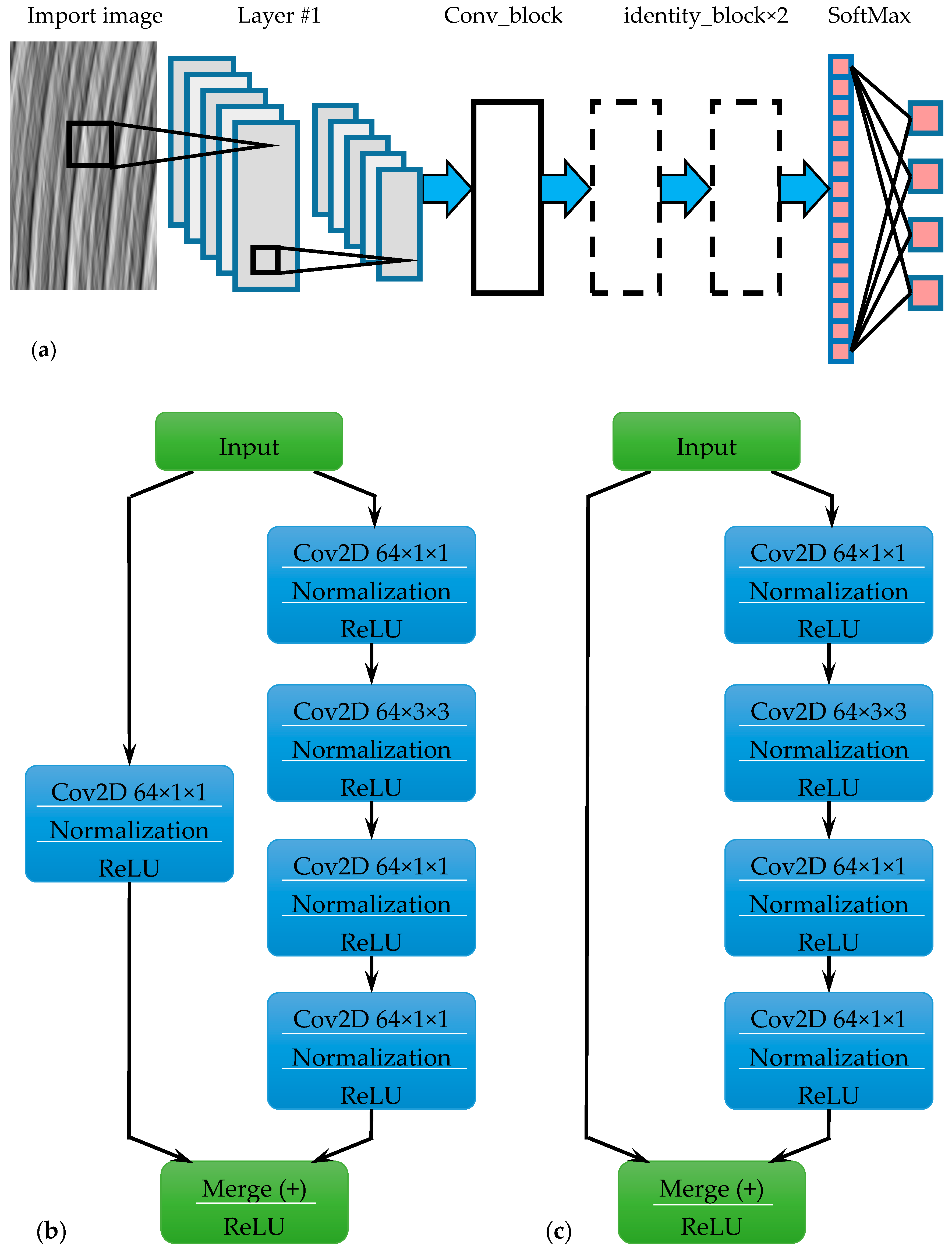
3.5. Network Architectures
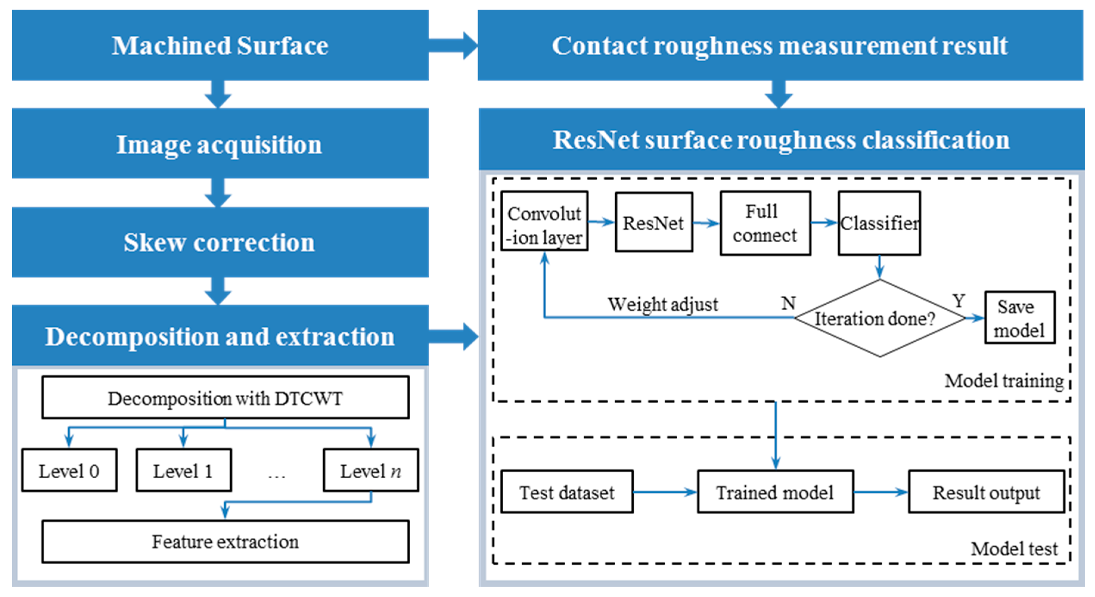
4. The Proposed Intelligent Surface Roughness Estimation Method
5. Surface Roughness Estimation
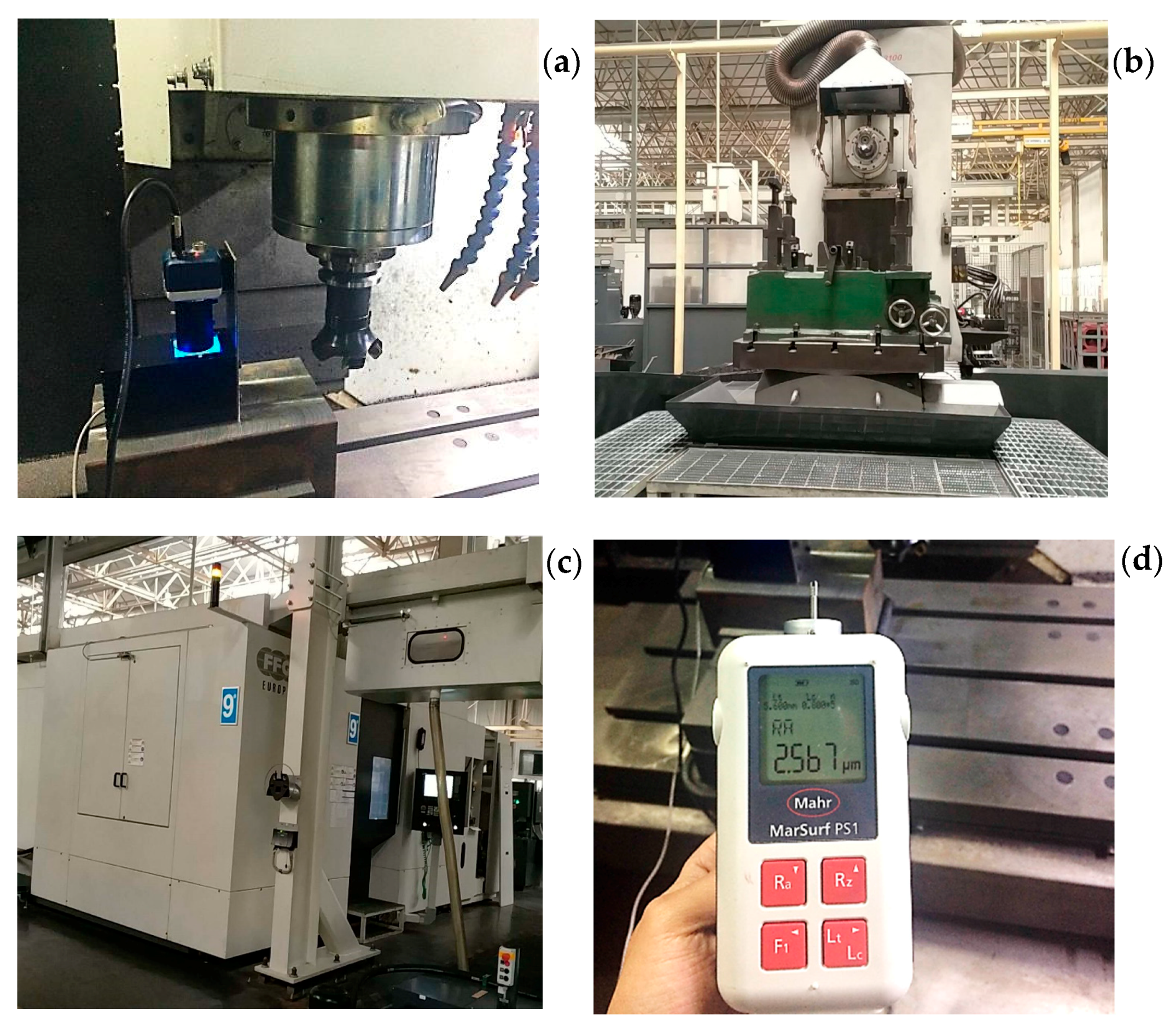
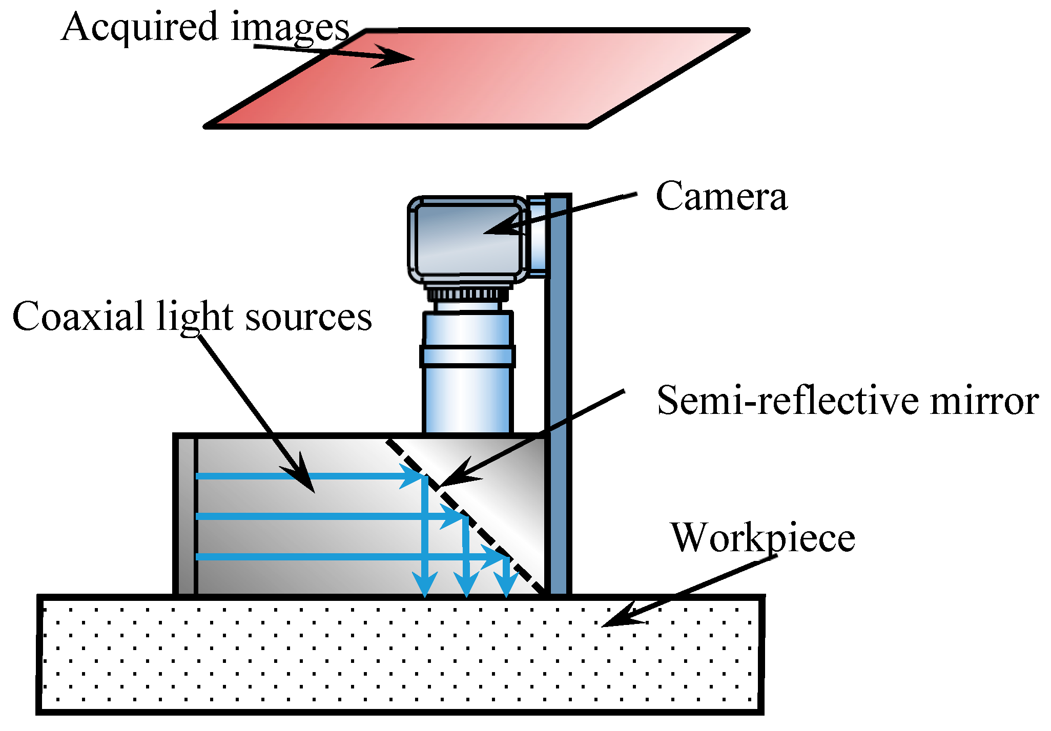
5.1. Experiment and Data Acquisition
5.2. Surface Roughness Classification
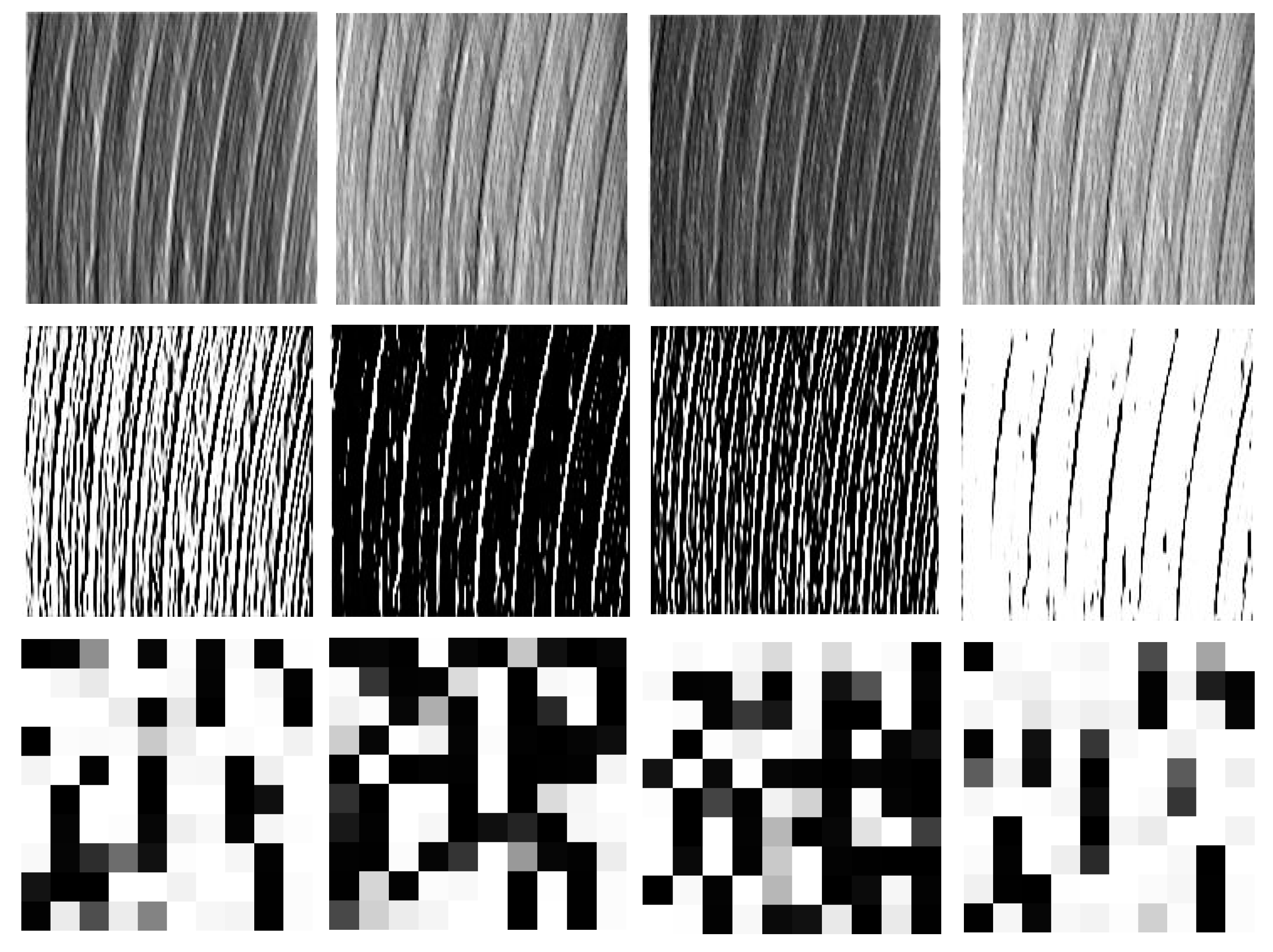
5.3. Texture Skew Correction and DTCWT Filtering
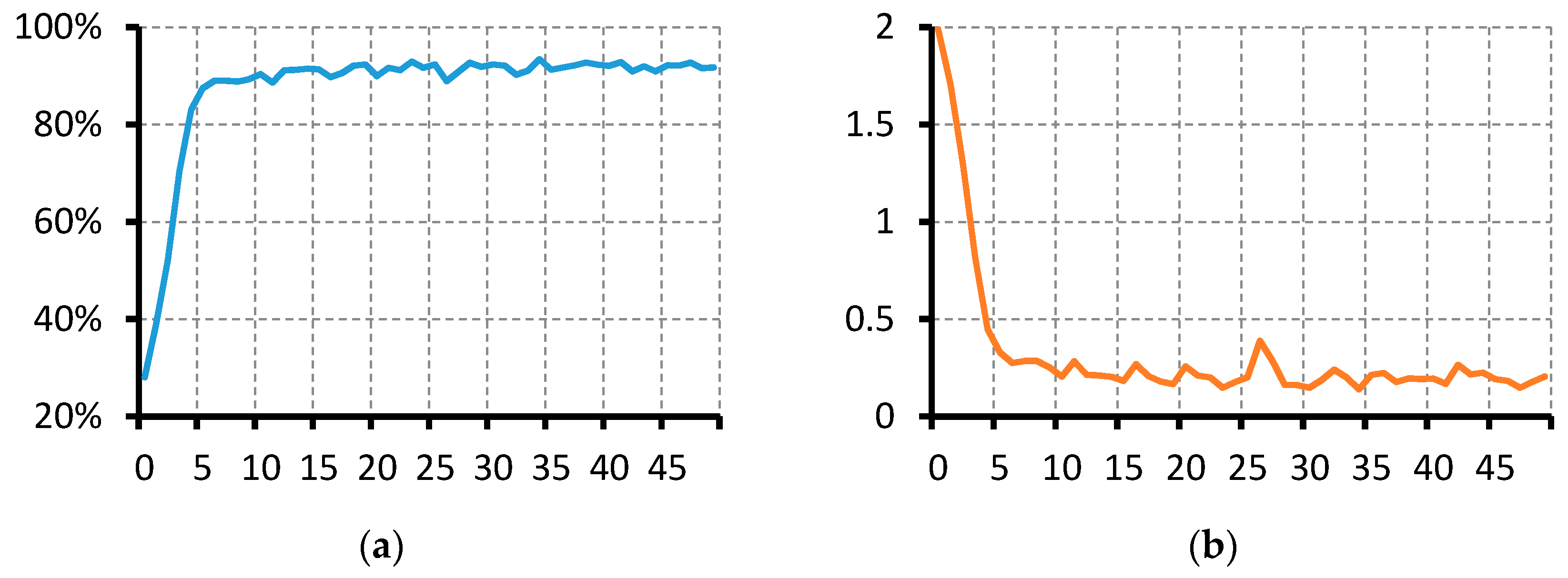
5.4. Network Training
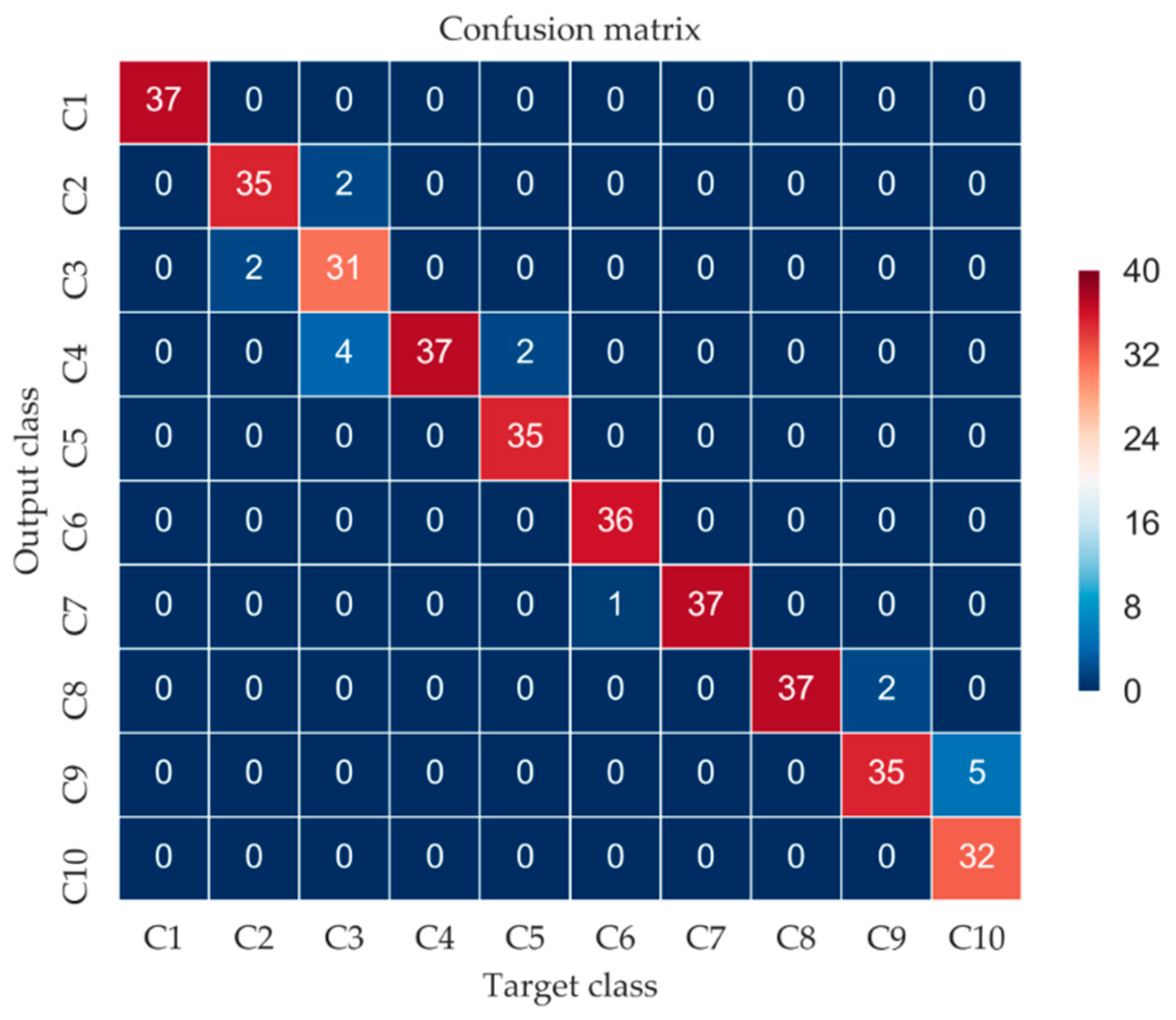
5.5. Experiment Results
- Precision = TP/TP + FP
- Recall = TP/TP + FN
- F1 Score = 2 × (Recall × Precision)/(Recall + Precision)
6. Discussion and Comparison
7. Conclusions
- (1)
- ResNet has proven to be an effective method for the surface roughness evaluation. Compared with traditional surface roughness measuring methods, the proposed method is a non-contact one without additional surface damages on the workpiece. Because of the engagement of ResNet in feature learning, this model does not rely on prior knowledge.
- (2)
- Surface milling experiments show that the proposed texture skew correction method is a feasible way to adjust image variabilities.
- (3)
- Effectiveness of the proposed novel method is verified by the surface roughness estimation on milled components. Results indicate that this method can distinguish different surface roughness classes with high precision.
- (4)
- Analysis of filters has demonstrated the function networks can be regarded as an automatic and intelligent realization of comparison specimen based manual surface roughness estimation. Despite similarities in principle the proposed method is also not sensitive to ambient light and does not rely on staffs’ experience. Therefore, it can be served as a superior alternative scheme for this task.
Acknowledgments
Author Contributions
Conflicts of Interest
References
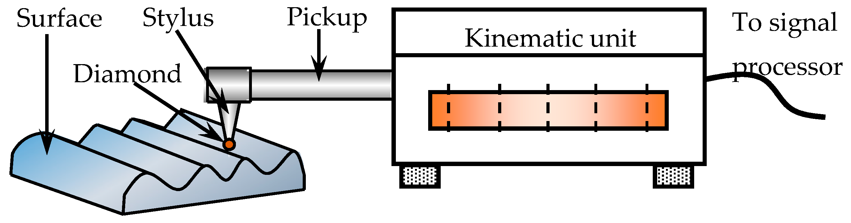
- Krehel’, R.; Pollák, M. The contactless measuring of the dimensional attrition of the cutting tool and roughness of machined surface. Int. J. Adv. Manuf. Technol. 2016, 60, 1–13. [Google Scholar] [CrossRef]
- Schmähling, J.; Hamprecht, F.A.; Hoffmann, D.M.P. A three-dimensional measure of surface roughness based on mathematical morphology. Int. J. Mach. Tools Manuf. 2006, 46, 1764–1769. [Google Scholar] [CrossRef]
- Huaian, Y.I.; Jian, L.I.U.; Enhui, L.U.; Peng, A.O. Measuring grinding surface roughness based on the sharpness evaluation of colour images. Meas. Sci. Technol. 2016, 27, 025404. [Google Scholar] [CrossRef]
- Quinsat, Y.; Tournier, C. In situ non-contact measurements of surface roughness. Precis. Eng. 2012, 36, 97–103. [Google Scholar] [CrossRef]
- Duboust, N.; Ghadbeigi, H.; Pinna, C.; Soberanis, A.; Collis, A.; Scalfe, R.; Kerrigan, K. An optical method for measuring surface roughness of machined carbon fibre-reinforced plastic composites. J. Compos. Mater. 2016, 51, 289–302. [Google Scholar] [CrossRef]
- Poon, C.Y.; Bhushan, B. Comparison of surface roughness measurements by stylus profiler, AFM and non-contact optical profiler. Wear 1995, 190, 76–88. [Google Scholar] [CrossRef]
- He, W.; Zi, Y.; Chen, B.; Wu, F.; He, Z. Automatic fault feature extraction of mechanical anomaly on induction motor bearing using ensemble super-wavelet transform. Mech. Syst. Signal Process. 2015, 54–55, 457–480. [Google Scholar] [CrossRef]
- Whitehead, S.A.; Shearer, A.C.; Watts, D.C.; Wilson, N.H. Comparison of methods for measuring surface roughness of ceramic. J. Oral Rehabil. 1995, 22, 421–427. [Google Scholar] [CrossRef] [PubMed]
- Launhardt, M.; Wörz, A.; Loderer, A.; Laumer, T.; Drummer, D.; Hausotte, T.; Schmidt, M. Detecting surface roughness on SLS parts with various measuring techniques. Polym. Test. 2016, 53, 217–226. [Google Scholar] [CrossRef]
- Jian, Z.; Jin, Z. Surface Roughness Measure Based on Average Texture Cycle. In Proceedings of the International Conference on Intelligent Human-Machine Systems and Cybernetics, Nanjing, China, 26–28 August 2010; IEEE: Piscataway, NJ, USA, 2010; pp. 298–302. [Google Scholar]
- Koçer, E.; Horozoğlu, E.; Asiltürk, I. Noncontact surface roughness measurement using a vision system. Proc. SPIE Int. Soc. Opt. Eng. 2015, 9445, 944525. [Google Scholar]
- Lee, W.K.; Ratnam, M.M.; Ahmad, Z.A. Detection of fracture in ceramic cutting tools from workpiece profile signature using image processing and fast Fourier transform. Precis. Eng. 2015, 44, 131–142. [Google Scholar] [CrossRef]
- Lee, W.K.; Ratnam, M.M.; Ahmad, Z.A. Detection of chipping in ceramic cutting inserts from workpiece profile during turning using fast Fourier transform (FFT) and continuous wavelet transform (CWT). Precis. Eng. 2017, 47, 406–423. [Google Scholar] [CrossRef]
- Verma, R.N.; Malik, L.G. Review of Illumination and Skew Correction Techniques for Scanned Documents. Proc. Comput. Sci. 2015, 45, 322–327. [Google Scholar] [CrossRef]
- Zhang, F.; Zhang, Y.; Qu, X.; Liu, B.; Zhang, R. Scanned Document Images Skew Correction Based on Shearlet Transform. Multi-Disciplinary Trends in Artificial Intelligence; Springer: Berlin/Heidelberg, Germany, 2015. [Google Scholar]
- Li, W.; Breier, M.; Merhof, D. Skew correction and line extraction in binarized printed text images. In Proceedings of the IEEE International Conference on Image Processing, Quebec City, QC, Canada, 27–30 September 2015; IEEE: Piscataway, NJ, USA, 2015; pp. 472–476. [Google Scholar]
- Shafii, M.; Sid-Ahmed, M. Skew detection and correction based on an axes-parallel bounding box. Int. J. Doc. Anal. Recognit. 2015, 18, 59–71. [Google Scholar] [CrossRef]
- Sun, W.; Chen, B.; Yao, B.; Cao, X.; Feng, W. Complex wavelet enhanced shape from shading transform for estimating surface roughness of milled mechanical components. J. Mech. Sci. Technol. 2017, 31, 823–833. [Google Scholar] [CrossRef]
- Silver, D.; Huang, A.; Maddison, C.J.; Guez, A.; Sifre, L.; Van Den Driessche, G.; Schrittwieser, J.; Antonoglou, I.; Panneershelvam, V.; et al. Mastering the game of Go with deep neural networks and tree search. Nature 2016, 529, 484–489. [Google Scholar] [CrossRef] [PubMed]
- Wang, F.-Y.; Zhang, J.J.; Zheng, X.; Wang, X.; Yuan, Y.; Dai, X.; Zhang, J.; Yang, L. Where does AlphaGo go: From Church-Turing thesis to AlphaGo thesis and beyond. IEEE/CAA J. Autom. Sin. 2016, 3, 113–120. [Google Scholar]
- Zeng, X.; Liao, Y.; Li, W. Gearbox fault classification using S-transform and convolutional neural network. In Proceedings of the 2016 10th International Conference on Sensing Technology (ICST), Nanjing, China, 11–13 November 2016; IEEE: Piscataway, NJ, USA, 2016; pp. 1–5. [Google Scholar]
- He, W.; Ding, Y.; Zi, Y.; Selesnick, I.W. Repetitive transients extraction algorithm for detecting bearing faults. Mech. Syst. Signal Process. 2017, 84, 227–244. [Google Scholar] [CrossRef]
- Hua, Y.; Tian, H. Depth estimation with convolutional conditional random field network. Neurocomputing 2016, 214, 546–554. [Google Scholar] [CrossRef]
- Zhu, Y.; Zhang, C.; Zhou, D.; Wang, X.; Bai, X.; Liu, W. Traffic sign detection and recognition using fully convolutional network guided proposals. Neurocomputing 2016, 214, 758–766. [Google Scholar] [CrossRef]
- Cira, F.; Arkan, M.; Gumus, B. Detection of Stator Winding Inter-Turn Short Circuit Faults in Permanent Magnet Synchronous Motors and Automatic Classification of Fault Severity via a Pattern Recognition System. J. Electr. Eng. Technol. 2016, 11, 416–424. [Google Scholar] [CrossRef]
- He, K.; Zhang, X.; Ren, S.; Sun, J. Deep Residual Learning for Image Recognition. In Proceedings of the 2016 IEEE Conference on Computer Vision and Pattern Recognition (CVPR), Las Vegas, NV, USA, 27–30 June 2016; IEEE: Piscataway, NJ, USA, 2016; pp. 770–778. [Google Scholar]
- Gong, Y.; Wang, L.; Guo, R.; Lazebnik, S. Multi-scale orderless pooling of deep convolutional activation features. In Proceedings of the 2014 European Conference on Computer Vision Computer Vision (ECCV), Zurich, Swiss, 6–12 September 2014; Springer: Berlin/Heidelberg, Germany, 2014; pp. 392–407. [Google Scholar]
- Singh, S.; Saini, A.K.; Saini, R.; Mandal, A.S.; Shekhar, C.; Vohra, A. A novel real-time resource efficient implementation of Sobel operator-based edge detection on FPGA. Int. J. Electr. 2014, 101, 1705–1715. [Google Scholar] [CrossRef]
- Shi, T.; Kong, J.; Wang, X.; Liu, Z.; Zheng, G. Improved Sobel algorithm for defect detection of rail surfaces with enhanced efficiency and accuracy. J. Cent. South Univ. 2016, 23, 2867–2875. [Google Scholar] [CrossRef]
- Duda, R.O. Use of the Hough transformation to detect lines and curves in pictures. Commun. ACM 1972, 15, 11–15. [Google Scholar] [CrossRef]
- Chen, B.; Zhang, Z.; Zi, Y.; He, Z.; Sun, C. Detecting of transient vibration signatures using an improved fast spatial–spectral ensemble kurtosis kurtogram and its applications to mechanical signature analysis of short duration data from rotating machinery. Mech. Syst. Signal Process. 2013, 40, 1–37. [Google Scholar] [CrossRef]
- Chen, B.; Zhang, Z.; Zi, Y.; He, Z. Novel Ensemble Analytic Discrete Framelet Expansion for Machinery Fault Diagnosis. J. Mech. Eng. 2014, 50, 77–86. [Google Scholar] [CrossRef]
- Duan, Y.; Liu, F.; Jiao, L.; Zhao, P.; Zhang, L. SAR Image segmentation based on convolutional-wavelet neural network and markov random field. Pattern Recognit. 2017, 64, 255–267. [Google Scholar] [CrossRef]
- Tan, Y.; Tang, P.; Zhou, Y.; Luo, W.; Kang, Y.; Li, G. Photograph aesthetical evaluation and classification with deep convolutional neural networks. Neurocomputing 2017, 228, 165–175. [Google Scholar] [CrossRef]
- Han, Y.; Lee, S.; Nam, J.; Lee, K. Sparse feature learning for instrument identification: Effects of sampling and pooling methods. J. Acoust. Soc. Am. 2016, 139, 2290–2298. [Google Scholar] [CrossRef] [PubMed]
- Kingma, D.; Ba, J. Adam: A method for stochastic optimization. In Proceedings of the International Conference on Learning Reprresentations, San Diego, CA, USA, 7–9 May 2015. [Google Scholar]
- Qin, P.; Xu, W.; Guo, J. An empirical convolutional neural network approach for semantic relation classification. Neurocomputing 2016, 190, 1–9. [Google Scholar] [CrossRef]
- Sun, W.; Yao, B.; Zeng, N.; Chen, B.; He, Y.; Cao, X.; He, W. An Intelligent Gear Fault Diagnosis Methodology Using a Complex Wavelet Enhanced Convolutional Neural Network. Materials 2017, 10, 790. [Google Scholar] [CrossRef] [PubMed]
- Chen, Z.Q.; Li, C.; Sanchez, R.V. Gearbox Fault Identification and Classification with Convolutional Neural Networks. Shock Vib. 2015, 2015, 390134. [Google Scholar] [CrossRef]
- Hensman, P.; Masko, D. The Impact of Imbalanced Training Data for Convolutional Neural Networks; KTH Royal Institute of Technology: Stockholm, Sweden, 2015. [Google Scholar]
- Yao, B.; Sun, W.; Chen, B.; Zhou, T.; Cao, X. Surface reconstruction based on the camera relative irradiance. Int. J. Distrib. Sens. Netw. 2018, 14, 1–9. [Google Scholar] [CrossRef]
- Ma, J.; Sun, L.; Wang, H.; Zhang, Y.; Aickelin, U. Supervised Anomaly Detection in Uncertain Pseudoperiodic Data Streams. ACM Trans. Internet Technol. 2016, 16, 1–20. [Google Scholar] [CrossRef]


| Property | VMC650E/850E | XK63100 | NBH800 |
|---|---|---|---|
| Milling mode | Down milling | Up milling | Up milling |
| Milling tool | Carbide disc milling tool | Carbide disc milling tool | Carbide disc milling tool |
| Feeding speed | 200 mm/min | 500 mm/min | 700 mm/min |
| Spindle speed | 960 rpm | 450 rpm | 2228 rpm |
| Cutting depth | 0.5 mm | 4 mm | 0.5 mm |
| Property | Information |
|---|---|
| Exposure time | 150 ms 10 μs |
| Gamma | 0 |
| Goal | 49 |
| Gain | 1.375× |
| Saturation | 100 |
| Roughness | Original Sample Number | Adjusted Sample Number | Label |
|---|---|---|---|
| [−Inf, 0.957) | 308 | 370 | C1 |
| [0.957, 1.67) | 152 | 370 | C2 |
| [1.67, 2.38) | 100 | 370 | C3 |
| [2.38, 3.1) | 135 | 370 | C4 |
| [3.1, 3.81) | 120 | 370 | C5 |
| [3.81, 4.52) | 200 | 370 | C6 |
| [4.52, 5.24) | 365 | 370 | C7 |
| [5.24, 5.95) | 370 | 370 | C8 |
| [5.95, 6.66) | 190 | 370 | C9 |
| [6.66, ) | 100 | 370 | C10 |
| Parameters | C1 | C2 | C3 | C4 | C5 | C6 | C7 | C8 | C9 | C10 | Mean |
|---|---|---|---|---|---|---|---|---|---|---|---|
| Precision | 1 | 0.95 | 0.94 | 0.86 | 1 | 1 | 0.97 | 0.95 | 0.88 | 1 | 0.95 |
| Recall | 1 | 0.95 | 0.84 | 1 | 0.95 | 0.97 | 1 | 1 | 0.95 | 0.86 | 0.95 |
| F1 score | 1 | 0.95 | 0.89 | 0.93 | 0.97 | 0.99 | 0.99 | 0.97 | 0.91 | 0.93 | 0.95 |
| Method | Accuracy |
|---|---|
| The proposed method (Texture skew correction + 2D-DTCWT + ResNet) | 95.14% |
| 2D-DTCWT + ResNet | 74.62% |
| CNN with over 30 layers | 69.73% |
| Texture skew correction + ResNet | 79.88% |
| Texture skew correction + ResNet with 18 layers | 91.14% |
© 2018 by the authors. Licensee MDPI, Basel, Switzerland. This article is an open access article distributed under the terms and conditions of the Creative Commons Attribution (CC BY) license (http://creativecommons.org/licenses/by/4.0/).
Share and Cite
Sun, W.; Yao, B.; Chen, B.; He, Y.; Cao, X.; Zhou, T.; Liu, H. Noncontact Surface Roughness Estimation Using 2D Complex Wavelet Enhanced ResNet for Intelligent Evaluation of Milled Metal Surface Quality. Appl. Sci. 2018, 8, 381. https://doi.org/10.3390/app8030381
Sun W, Yao B, Chen B, He Y, Cao X, Zhou T, Liu H. Noncontact Surface Roughness Estimation Using 2D Complex Wavelet Enhanced ResNet for Intelligent Evaluation of Milled Metal Surface Quality. Applied Sciences. 2018; 8(3):381. https://doi.org/10.3390/app8030381
Chicago/Turabian StyleSun, Weifang, Bin Yao, Binqiang Chen, Yuchao He, Xincheng Cao, Tianxiang Zhou, and Huigang Liu. 2018. "Noncontact Surface Roughness Estimation Using 2D Complex Wavelet Enhanced ResNet for Intelligent Evaluation of Milled Metal Surface Quality" Applied Sciences 8, no. 3: 381. https://doi.org/10.3390/app8030381