Path Planning Strategy for Vehicle Navigation Based on User Habits

Abstract

Vehicle navigation is widely used in path planning of self driving travel, and it plays an increasing important role in people's daily trips. Therefore, path planning algorithms have attracted substantial attention. However, most path planning methods are based on public data, aiming at different driver groups rather than a specific user. Hence, this study proposes a personalized path decision algorithm that is based on user habits. First, the categories of driving characteristics are obtained through the investigation of public users, and the clustering results corresponding to the category space are obtained by log fuzzy C-means clustering algorithm (LFCM) based on the driving information contained in the log trajectories. Then, the road performance personalized quantization algorithm evaluation is proposed to evaluate roads from the user’s field of vision. Finally, adaptive ant colony algorithm is improved and used to validate the path planning based on the road performance personalized values. Results show that the algorithm can meet the personalized requirements of the user path selection in the path decision.

1. Introduction

With the rapid development of the modern automobile industry, self-driving groups are steadily increasing and road traffic pressure is increasing. These changes do not match users’ demand for comfortable travel. In addition to the expansion of existing road networks, attempts have been made to avoid the clustering effect caused by the planning of the integration of personalized travel path for users. For example, the full use of existing resources in public transportation can ease traffic pressure and improve user experience in personalized travel. Therefore, studying the personalized paths of users is of great social and economic significance.

Mature navigation systems and path planning algorithms mainly focus on the fastest path [1,2,3,4], the shortest path [5,6,7,8] or the most comfortable path [4,9] between specified starting and target points. In recent years, path optimization algorithms of multi-objective optimization [10,11,12,13,14] and single-objective optimization [15,16], as well as a few traffic impact factors, have deepened [17,18] and popular routes planning [19,20]. Moreover, significant attention has been directed toward personalized path guidance systems. Campigotto P [20] introduces the favorite route recommendation (FAVOUR) approach to provide a personalized, situation-aware route based on the information updating through Bayesian learning, which was obtained from initial configuration files (home location, work place, mobility options, etc.). A personalized fuzzy path planning algorithm based on the fuzzy sorting of the center of gravity was proposed by Nadi [21], in which a optimization route according to user standard types was formulated through analyzing the uncertainty of user preferences through the expression of fuzzy linguistic preference relations. A personalized recommendation route algorithm based on large trajectory data was proposed by Dai J [22] where both drivers’ driving preferences and multiple travel costs were considered to recommend personalized routes to individual drivers, however, the shortcoming was that the trajectory data were based on public drivers. A trip router planning method with individualized preferences was proposed by Letchner J [23] which presents a set of methods for including driver preferences and time-variant traffic condition estimates during route planning. Zhu X [24] put forward a personalized and time-sensitive route recommendation system, in which user preferences and time information were acquired through location-based social network where users’ location and access information was shared by different users. Qiong Long [25] proposed a dynamic route guidance method for drivers’ personalized needs where a qualitative and personalized evaluation was conducted on road networks with consideration of preferences according to the premise of obtaining user preferences, and then Dijkstra algorithm was used to find the optimal path.

The aforementioned results lay a good theoretical foundation; however, there still exist three shortcomings: (1) the personalized path planning algorithm is aimed at different driver groups but not at a specific user; (2) driver feature data are based on public trajectories or public information, which leads to the lack of pertinence; and (3) personalized performance values fail to be obtained in the evaluation of road traffic network performance.

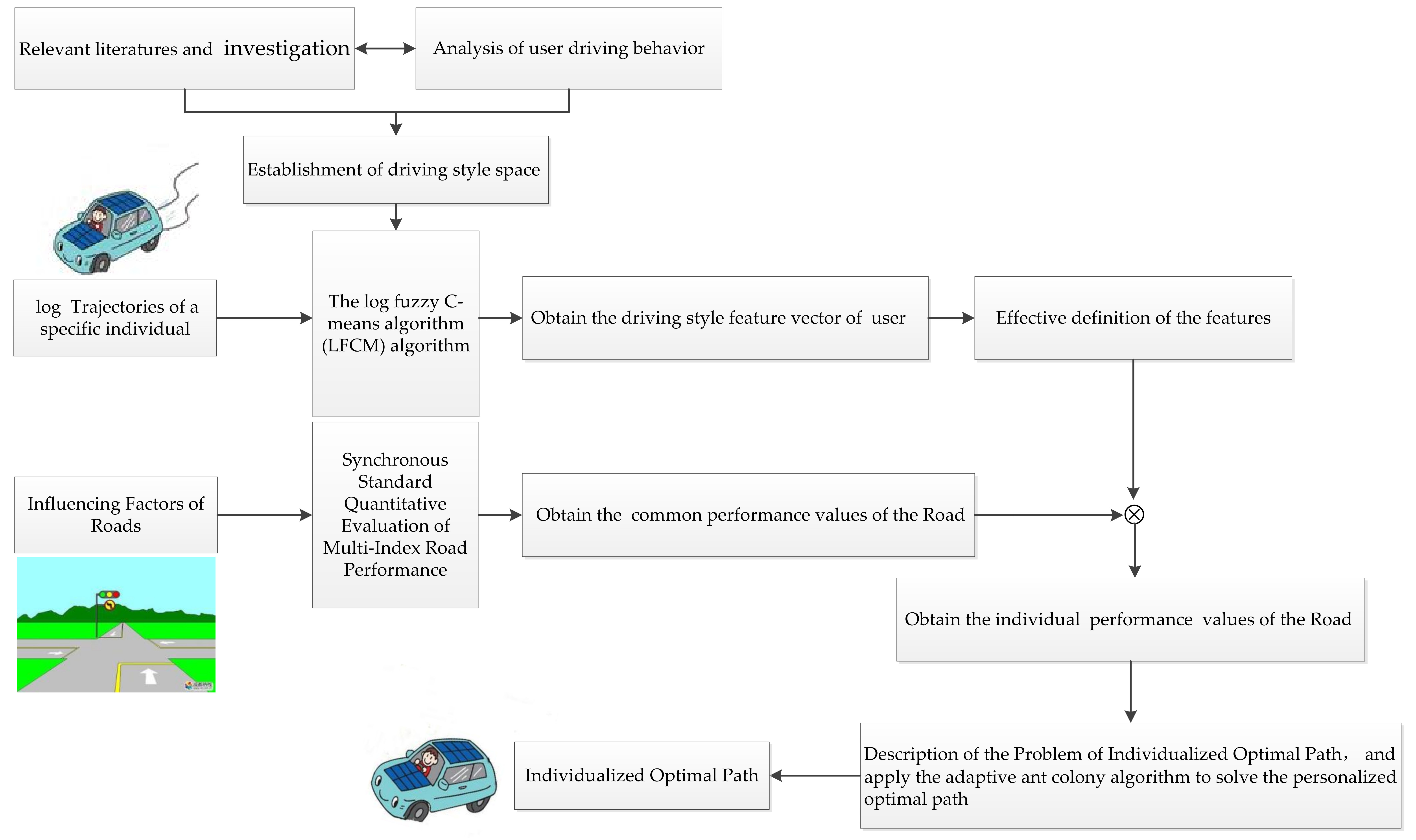
Hence, to the best of our knowledge, this paper explores the possibility of providing a higher level of personalized path planning using trajectory information. Specifically, three major contributions have been made and structured as follows. First, a log C-means clustering algorithm (LFCM) is introduced in Section 2.1 to lead the characteristic mining and clustering process of a specific user who provides the log trajectories. Second, an individualized quantitative evaluation system of road performance is built in Section 2.2 to obtain specific performance value in the view of the owner of the log tracks. Third, adaptive ant colony algorithm is improved and utilized to validate the path planning based on the personalized road values in Section 2.3 to find the optimal individualized path.

2. Materials and Methods

2.1. Mining and Clustering of Users’ Driving Habits

2.1.1. Establishment of Driving Style Space

Driving style space should be analyzed before driver style clustering to ensure the rationality and reliability of the results of the LFCM. A driver can choose from a wide selection of varied details, generally, including time-saving [1,2,3], economic [26,27] and comfort [4,9]. For ease of discussion, we record the set of three indicators above as a style space. For most users, the style features are not limited to a single element of the style space, but a coexistence of multiple coupling indexes, whose index weight varies in each individual.

2.1.2. Acquisition of Individualized Driving Styles

Based on the fuzzy C-means algorithm [28], we integrate driving behavior characteristics and introduce the log fuzzy C-means algorithm (LFCM) to guide the clustering of driving characteristics in the style space. The LFCM algorithm is shown in Figure 1.

• Selection of style clustering center

(1)

Mining of driving characteristics

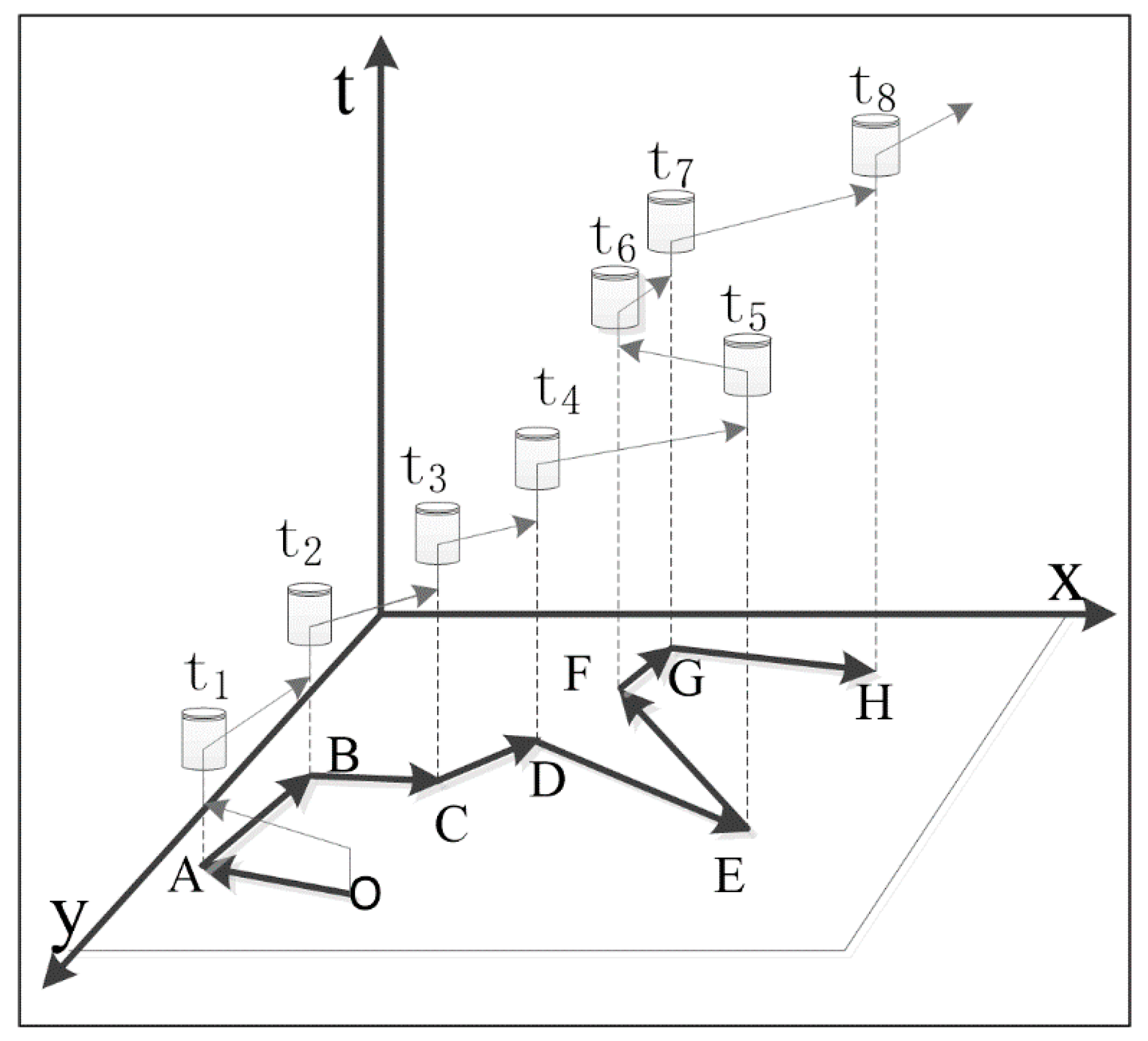
Driving characteristics in log trajectories should be mined [29] before the core process of feature clustering. Here, space–time paths of time geography [30] are used to excavate the driving characteristics (Figure 2), in which the two-dimensional coordinates represent the historical space position of the vehicle, while the vertical coordinates indicate the time of the vehicle arriving at the corresponding space position.

The relationships among the speed of driving $v_t$ at any time $t$, the acceleration of driving $a_t$, and the tangent slope of the inclined curve $k_t$ is shown in Formulas (1) and (2).

$$v_t=\frac{1}{k_t}$$

(1)

$$a_t=\underset{\tau \to t}{\lim }\frac{\frac{1}{k_{\tau }}-\frac{1}{k_t}}{\tau -t}$$

(2)

The total square root acceleration of the total weight $a_v$ in ISO2631 is used to approximate the comfort level of the human body; it is defined as follows:

$$a_v={\left({\lambda }_x^2{a}_x^2+{\lambda }_y^2{a}_y^2+{\lambda }_z^2{a}_z^2\right)}^{\frac{1}{2}}$$

(3)

where $a_x,a_y,a_z,{\lambda }_x,{\lambda }_y,\mathrm{and}{\lambda }_z$, respectively, represent the square root acceleration and the direction factors in the forward, horizontal, and vertical directions of the vehicle. The comparison between the root acceleration of the total weight of different values and the comfort level of the human body is shown in

Table 1. Corresponding relation between acceleration and comfort level.

Total Vibration av/m·s−2	Time Feature Weight ωt
<0.315	Without malaise
0.315–0.63	Slightly uncomfortable
0.5–1	Quite uncomfortable
0.8–1.6	Uncomfortable
51.25–2.5	Extremely uncomfortable
>2	Terrible

.

The quality of the natural environment has a significant impact on the outcome of a user’s path selection. The definition of the evaluation index is

$$I={\displaystyle \sum _{i=1}^m{I}_i}={\displaystyle \sum _{i=1}^m\frac{C_i}{S_i}}$$

(4)

where $I_i,C_i,\mathrm{and}{S}_i$ represent the environmental quality index, coverage rate, and evaluation standard of the natural environment factors $i$; $m$ is the species number of $i$, including the road greening rate, river distribution, and air quality; and $I$ denotes positive correlation with the comprehensive road environment.

(2)

Selection of cluster center

To minimize the clustering convergence time and avoid the local optima [31,32] before the clustering of characteristics, we must fully utilize the human inductive ability to restrict and select the value of the initial cluster center. The following principles are adopted for selecting the time, economic value, and comfort index of the cluster center.

Time clustering center: $v\ge v_0,\left|a\right|\ge \left|a_0\right|$, where $v_0,a_0$ according depend on adjustments to a specific situation.

Economic cluster center: $\left|a\right|\le \left|a_0\right|,c_0\to c_{0·\min }$, where $c_0$ represents the consumption rate for oil and facilities, and $c_{0·\min }$ represents the minimum consumption rate for fuel and facilities.

Comfort clustering center: $\left|a_v\right|\le \left|a_{v0}\right|,I\ge I_0$, where $a_{v0}$ is routinely specified as 0.63 while $I_0$ is adjusted according to user requirements.

(3)

Improved fuzzy C-means clustering

The minimum element, which contains the driving characteristics, is defined as the vector eigenvalue and is called the vector element. The Hausdorff distance [33,34,35,36] of each vector element to the time, economy, and comfort clustering centers is calculated, and the contribution of driving information to three different driving styles is measured. The fuzzy C-means algorithm is used to complete the clustering of the characteristics of each vector element. The concrete steps are as follows.

Step 1: A three-dimensional cluster coordinate system is established based on driving speed, consumption rate for fuel and facilities, total root mean square acceleration, and integrated environmental quality. The time, economic, and comfort information contained in each log vector element are expressed in the cluster coordinate system.

Step 2: According to the selection principle of clustering centers, the initial time, economic, and comfort clustering centers are ensured when constraint conditions are satisfied. In this way, the three cluster centers are moderately separated.

Step 3: The Hausdorff distance $d_{\mathrm{HD}}\left(f,o\right)$ of the log road vector element $f$ to the time, economy, and comfort cluster centers $O$ is calculated in Formula (5), where $F$ is the finite set of vector elements, and $O$ is the set of time, economy, and comfort clustering centers.

$$\{\begin{array}{l}{d}_{\mathrm{HD}}\left(f,o\right)=\min \left(h\left(F,\mathrm{O}\right),h\left(\mathrm{O},F\right)\right)\\ h\left(F,\mathrm{O}\right)=\underset{f\in F}{\max }\underset{o\in \mathrm{O}}{\min }d\left(f,o\right)\\ h\left(\mathrm{O},F\right)=\underset{o\in \mathrm{O}}{\max }\underset{f\in F}{\min }d\left(o,f\right)\end{array}$$

(5)

Step 4: The membership degree of each vector element $f$ to the three cluster centers is calculated in Formula (6).

$$R_{o\leftarrow f}=\frac{\mathrm{card}F/d_{\mathrm{HD}}^2\left(f,o\right)}{{\displaystyle \sum _{o\in \mathrm{O}}{\displaystyle \sum _{f\in F}\left(1/d_{\mathrm{HD}}^2\left(f,o\right)\right)}}}$$

(6)

Step 5: The vector elements of the time, economy, and comfort cluster centers are updated according to the membership degree, as shown in Formula (7).

$$o^{\prime }=\frac{{\displaystyle \sum _{f\in F}f•R_{o\leftarrow f}^2}}{{\displaystyle \sum _{f\in F}{R}_{o\leftarrow f}^2}}$$

(7)

Step 6: If the conditions shown in Formula (8) are satisfied, the iteration stops. Otherwise, the process returns to Step 2, where $O^{\prime }\mathrm{and}O$ represent the cluster center variables of the current time and the previous moment, respectively.

$$\underset{o\in \mathrm{O}}{\max }\{\Vert o^{\prime }-o\Vert \}<\epsilon$$

(8)

Step 7: Normalization is conducted according to Formula (9), where $j=\mathrm{t},\mathrm{m},\mathrm{c}$ represent the arbitrary sample time, economy, and comfort dimensions, respectively. ${\mathrm{s}}_{i\cdot j}{,\mathrm{s}}_{\min \cdot j}{,\mathrm{and}\mathrm{s}}_{\max \cdot j}$ represent the performance value, and the minimum and maximum performance values of sample $i$ underdimension $j$, respectively. $s_{i\cdot j}^{\ast }$ is the new performance value of sample $i$ under dimension $j$. after the normalization process.

$${\mathrm{s}}_{i·j}^{\ast }=\frac{{\mathrm{s}}_{i·j}-{\mathrm{s}}_{\min ·j}}{{\mathrm{s}}_{\max ·j}-{\mathrm{s}}_{\min ·j}}$$

(9)

The clustering results of the log road vector element features relative to the time (red), economic (green), and comfort (blue) cluster centers are shown in Figure 3.

• Sample screening and class-weighted combination

In the LFCM clustering, the validity of the statistics of the number of vectors in each cluster center directly affects the accuracy of driving style judgement. The effectiveness of each cluster center sample is as follows.

Step 1: The small effective ball radius $r_0$ is selected randomly (Figure 4a) to initialize the valid range of the sample. The corresponding plane projection of the valid ball is shown in Figure 4b.

Step 2: Taking the sample local density [33] and the Euclidean distance of the high-density point samples as the standard, the effective radius is adjusted positively according to Formula (10). The effective radius of clustering is finally determined as $r$. As shown in Figure 4c, the corresponding plane projection is shown in Figure 4d, where $d_{io}\mathrm{and}{d}_{ij}$ represent the Euclidean distance of sample $i$ to the cluster center $O$ and the high-density point sample $j$, respectively; $d_c$ is the truncated distance, which is related to the average percentage of the total sample size and number of neighbor sample points; ${\rho }_i\mathrm{and}{\rho }_i$ denote the local sample density of $i\mathrm{and}j$, respectively; ${\delta }_i$ is the shortest Euclidean distance between $i$ and the high-density point sample $j$; and $\tau \mathrm{and}\epsilon$ are both related boundary parameters which are often substitution of empirical value.

$$\{\begin{array}{l}{\rho }_i={\displaystyle \sum _{j=1}^{\mathrm{n}}\exp \left(-\frac{d_{ij}}{d_c^2}\right)}\ge \tau \\ {\delta }_i={\min }_{j:{\rho }_i>{\rho }_i}(d_{ij})\le \epsilon \end{array}$$

(10)

Step 3: The invalid samples of time, economic, and comfort cluster centers are deleted, as shown in Figure 4e. The corresponding plane projection is shown in Figure 4f. The number of samples within the effective radius $r$ of each cluster center is counted as $n_{\mathrm{t}},n_{\mathrm{m}},n_{\mathrm{c}}$.

Step 4: The distribution weight of time, economy, and comfort indexes is obtained through the normalization process shown in Formula (11).

$$\{\begin{array}{l}{\omega }_{\mathrm{T}}=\frac{n_{\mathrm{t}}}{n_{\mathrm{t}}+n_{\mathrm{e}}+n_{\mathrm{c}}}\\ {\omega }_{\mathrm{M}}=\frac{n_{\mathrm{e}}}{n_{\mathrm{t}}+n_{\mathrm{e}}+n_{\mathrm{c}}}\\ {\omega }_{\mathrm{C}}=\frac{n_{\mathrm{c}}}{n_{\mathrm{t}}+n_{\mathrm{e}}+n_{\mathrm{c}}}\end{array}$$

(11)

The user’s driving style feature vector is expressed as $W=\left[{\omega }_{\mathrm{T}},{\omega }_{\mathrm{M}},{\omega }_{\mathrm{C}}\right]$.

2.2. Individualized Quantitative Evaluation of Road Performance

2.2.1. Analysis of Influencing Factors of Roads

Road and its subsidiary factors [25,37,38], including peripheral environment, traffic laws and regulations, driver factors and other dynamic factors, whose varied details are listed in

Table 2. Influencing factors of roads.

Factor Types		Influence Factor
Road factors	road self-factors	road alignment, road length, road intersection number, road level, road width, number of continuous turns, road evenness, isolation of green belts, and scribing isolation. the ratio of green to credit, road traffic density, road evenness, number of crossings, average speed of main roads, blocking rate of intersections, average traffic delays and illegal occupancy Lane rates.
	Peripheral environmental factors	road greening and landscape organization gas station, parking lot, traffic indicator, trunk road lighting rate, parking guidance and traffic guidance system setting garbage field and operation station, pedestrian crossing facilities, to sign and rate of population density circulation area
Subsidiary factors	law and regulation factors	internship high speed limit speed limit, limit height, weight limit, restriction entry single line setting, single and double number limit line influence, restriction, or prohibition of area and type of vehicle on the time of road separation
	Driver factors	restrictions on driving ability drive-age limit
	Other dynamic factors	the fluctuation of the driver’s mood emergency (large-scale mass activities, major traffic accidents, temporary traffic control) occupation rate weather, natural calamities, urban construction

, can reflect road performance in different extents, and then affect user path selection results.

2.2.2. Synchronous Standard Quantitative Evaluation of Multi-Index Road Performance

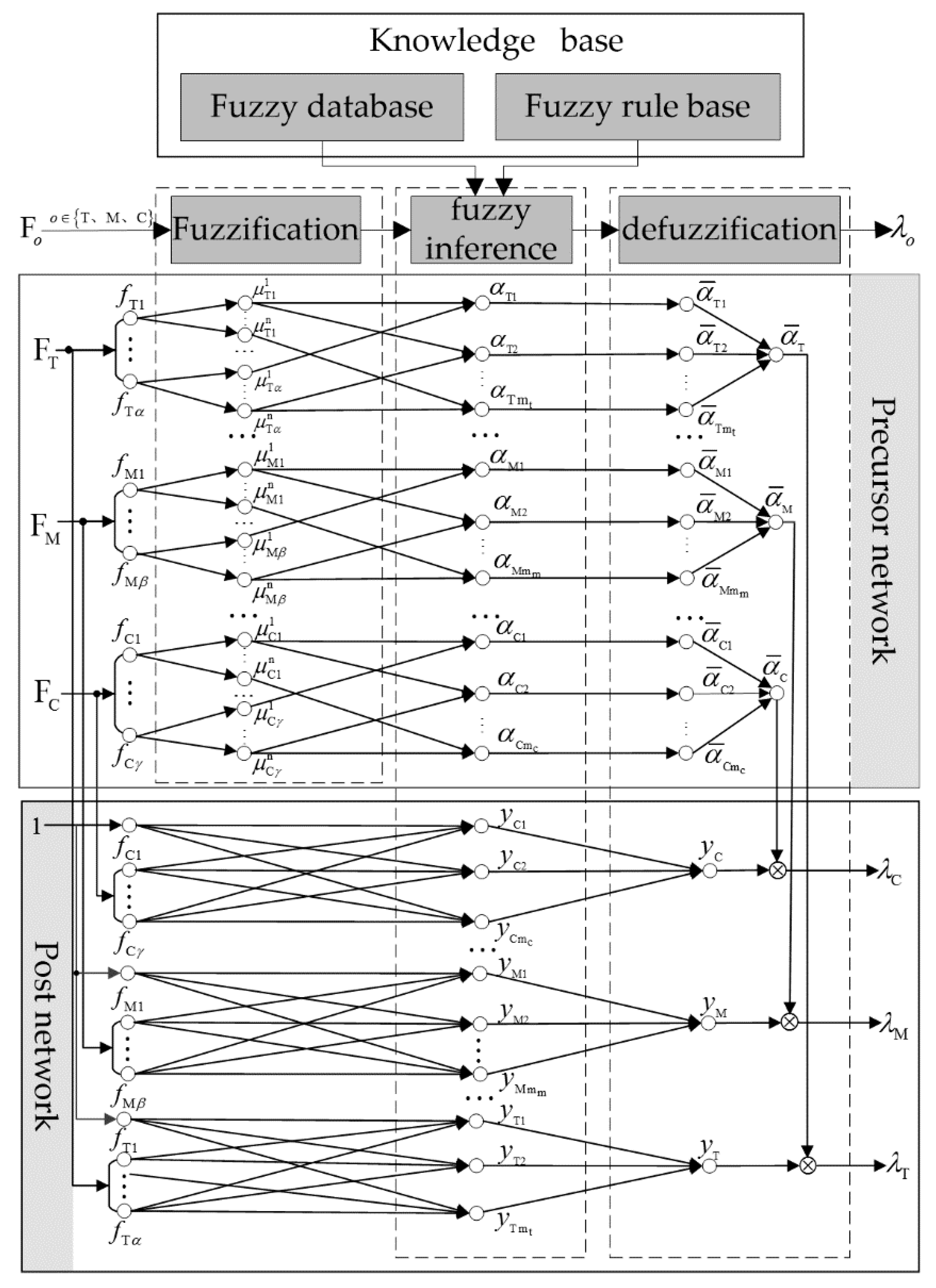
In this section, an accurate synchronous multi-index quantitative evaluation of road performance modeling system is established by maximizing the advantages of solving dimensions based on a T–S fuzzy neural network [39,40], whose architecture is shown in Figure 5.

The evaluation model using the “IF–THEN” form ${\mathrm{R}}^{\tau }$: $\mathrm{IF}{f}_{o1}\mathrm{is}{\mu }_{o1}^{i_1},f_{o2}\mathrm{is}{\mu }_{o2}^{i_2},\cdots f_{ok}\mathrm{is}{\mu }_{ok}^{i_k}$ $\mathrm{THEN}{y}_{o\tau }=p_{o0}^{i_1}+p_{o1}^{i_2}{f}_{o1}+p_{o2}^{i_3}{f}_{o2}+\cdots +p_{ok}^{i_k}{f}_{ok}$, where $o\in \{\mathrm{T},\mathrm{M},\mathrm{C}\},k\in \{\left|{\mathrm{F}}_{\mathrm{T}}\right|,\left|{\mathrm{F}}_{\mathrm{M}}\right|,\left|{\mathrm{F}}_{\mathrm{C}}\right|\}$ are the set of significant factors of time, economy, and comfort; $f_{oj}\in \left\{{\mathrm{F}}_{\mathrm{T}},{\mathrm{F}}_{\mathrm{M}},{\mathrm{F}}_{\mathrm{C}}\right\},j=1,2,\cdots k$, ${\mu }_{oj}^i$ is the fuzzy set of index $o$; and $p_{oj}^i$, y_oj denote the corresponding parameter and output of the fuzzy rule, respectively.

The former network is used to calculate the applicability of fuzzy rules. For any $f_{oj}$, the membership degree of the fuzzy layer is first based on the Gaussian membership function shown in Formula (12), where $a_j^i\mathrm{and}{b}_j^i$ represent the function centers and widths, respectively; $i=1,2,\dots ,n$ where $n$ is the fuzzy division number of $f_{oj}$. To satisfy the actual factors that affect the situation, $n$ is assumed to be seven levels that represent the seven effects of - - -, - -, -, 0, +, + +, and +++, respectively.

$${\mu }_{oj}^i=\exp \left(-{\left(f_{oj}-a_j^i\right)}^2/b_j^i\right)$$

(12)

Then, we calculate the fitness of each rule by using a multiplicative operator in the fuzzy reasoning layer, as shown in Formula (13).

$${\alpha }_{o\tau }={\mu }_{o1}^{i_1}·{\mu }_{o2}^{i_2}·{\mu }_{o3}^{i_3}·\cdots {\mu }_{ok}^{i_k}\left(\tau =1,2,\cdots ,n^k\right)$$

(13)

Finally, to avoid model turbulence caused by the order of magnitude of significant road influencing factors, we perform normalization in the anti-fuzzification layer, as shown in Formula (14).

$${\overline{\alpha }}_{o\tau }=\frac{{\alpha }_{o\tau }}{{\displaystyle \sum _{\mathrm{i}=1}^{{\mathrm{n}}^k}{\alpha }_{oi}}}$$

(14)

The post-part network consists of three sub-networks of the same structure for outputting fuzzy rules of time, economy, and comfort indexes. The input layer needs to be supplemented with a constant term, that is, input parameter 1 of the 0th node, which is used to generate the constant term in the road performance level calculation result. The fuzzy inference layer calculates the consequent of each fuzzy rule, as shown in Formula (15).

$$y_{o\tau }=p_{o0}^{i_1}+p_{o1}^{i_2}{f}_{o1}+p_{o2}^{i_3}{f}_{o2}+\cdots +p_{ok}^{i_k}{f}_{ok}$$

(15)

The output of the network is the weighted sum of the fuzzy rules, as shown in Formula (16). The weighting coefficient is the applicability of the rules and the result of the road performance level after the output-clarified process.

$${\lambda }_o={\overline{\alpha }}_o\otimes y_o={\displaystyle \sum _{\tau =1}^{{\mathrm{n}}^k}{\overline{\alpha }}_{o\tau }{y}_{o\tau }}$$

(16)

According to the equilibrium characteristics of the weight distribution of a user’s driving style, the overall characteristics of different path tendencies based on user choice is divided into three categories, as shown in the first four columns of

Table 3. Driving style classification.

Style Type	ωt	ωm	ωc	Personal-Value ω
$c_3^1$	valid	—	—	ωTλT
	—	valid	—	ωMλM
	—	—	valid	ωcλc
$c_3^2$	valid	valid	—	ωTλT + ωMλM
	valid	—	valid	ωTλT + ωcλc
	—	valid	valid	ωMλM + ωcλc
$c_3^3$	valid	valid	valid	ωTλT + ωMλM + ωcλc

, where $c_3^1,c_3^2,c_3^3$, respectively, represent the number of effective features in user eigenvectors.

In addition, to avoid excessive neutralization of the decision-making power of the high weight feature, and ensure the good consistency and universality of the quantitative and the actual evaluation results, an effective definition of the features is presented in Theorem 1.

Theorem 1.

For any vector element of the driving characteristics, if any of the following arbitrary conditions are satisfied, the element can be called an invalid feature; otherwise, it is an effective feature.

(a)

${\omega }_0>0.35\times \max W$

(b)

${\bar{\omega }}_o>0.35\max W$ and ω_o ≥ 0.5* ${\bar{\omega }}_o$, where ${\bar{\omega }}_o$ = W − maxW − minW

The personalized quantitative evaluation of roads is a weighted summation of the effective characteristics and the corresponding road standard quantification values. The calculation process for the personalized road performance from a user perspective is shown in the last column of Table 3.

To facilitate the dynamic optimization of the follow-up path, we standardize the deviation of the personalized road performance ω, adjust the original performance values linearly, and adjust the road area range of the traffic network to [0, 1], as shown in Formula (17).

$${\omega }^{\ast }=\frac{\omega -{\omega }_{\min }}{{\omega }_{\max }-{\omega }_{\min }}$$

(17)

2.3. Dynamic Selection of Path

2.3.1. Description of the Problem of Individualized Optimal Path

To avoid the redundant consumption of roads and the interference of irrelevant paths, we introduce a linear transformation between road performance and road consumption. The use of road performance as an index is also avoided, as shown in Formula (18). For any two points in the road network, the optimal path [41] is solved based on the consumption value $\overline{\omega }\left(\overline{\omega }\in \left[0,1\right]\right)$.

$$\overline{\omega }=\frac{1}{{\omega }^{*}}$$

(18)

The optimal path problem is described as follows. Let $\mathrm{G}=\{V,L,\overline{W}\}$ be a road network digraph, where $V=\{1,2,\cdots n\}$ is a set of branch points of the road network, $L\subseteq V\times V$ is a set of roads of G, and $\overline{W}={\left({\overline{\omega }}_{ij}\right)}_{\left|L\right|\times \left|L\right|}$ is the set of consumption of roads. The path consumption of directed roads $\left(i,j\right)\in L$ between any connected branch points i and j is recorded as ${\overline{\omega }}_{ij}$, in which $i,j\in V;{\overline{\omega }}_{ij}\in \left[0,1\right]$. For $\forall \mathrm{A},\mathrm{B}\in V$, the optimal path is the path of minimum cumulative consumption from point A to point B in the road network digraph.

2.3.2. Global Dynamic Selection of Path

The adaptive ant colony algorithm proposed in the literature [42,43,44] adaptively controls the proportion of pheromone concentration in the current optimal solution and updates the global pheromone concentration of the optimal path in real time by introducing a hyperbolic sine function as an adaptive dynamic factor $\sigma \left(\sigma \in \left(0,1\right)\right)$. In this way, the path exploration results can be effectively implemented when the performance of each path is known. In view of the real-time changes in the characteristics of road traffic network status, we apply the adaptive ant colony algorithm to solve the personalized optimal path. We add dynamic updating links of road performance to simulate the road environment realistically. The flowchart of the improved adaptive ant colony algorithm and its contribution in this study are shown in Figure 6a,b (shadow), respectively.

3. Results

3.1. Emulation

To verify the proposed theory and the effectiveness of the algorithm, we use a road network environment with a 5 × 5 grid simulated according to ideal settings from top to bottom and from left to right in the order of the road traffic environment simulation. The grid performance simulation of traffic assignment, the network structure, and the performance simulation of road vector are shown in Figure 7 and

Table 4. The road performance of the analog road network.

Road Number	Standard Road Performance (λt, λm, λc)
1–12	[0.77,0.50,0.45],[0.34,0.74,0.38],[0.56,0.69,0.72],[0.49,0.59,0.21]
	[0.73,0.69,0.66],[0.66,0.60,0.78],[0.47,0.41,0.79],[0.21,0.37,0.67]
	[0.69,0.40,0.46],[0.47,0.52,0.50],[0.57,0.64,0.33],[0.68,0.39,0.59]
13–24	[0.75,0.70,0.39],[0.64,0.54,0.78],[0.31,0.42,0.64],[0.44,0.62,0.45]
	[0.76,0.53,0.65],[0.75,0.47,0.36],[0.45,0.62,0.46],[0.74,0.57,0.76]
	[0.23,0.68,0.61],[0.41,0.77,0.33],[0.69,0.51,0.70],[0.21,0.73,0.58]
25–36	[0.28,0.30,0.28],[0.32,0.79,0.32],[0.32,0.36,0.56],[0.56,0.35,0.58]
	[0.36,0.73,0.42],[0.32,0.64,0.55],[0.21,0.28,0.47],[0.65,0.21,0.23]
	[0.47,0.74,0.22],[0.76,0.32,0.39],[0.48,0.38,0.21],[0.45,0.60,0.43]
37–48	[0.71,0.37,0.61],[0.52,0.48,0.26],[0.32,0.24,0.22],[0.60,0.79,0.57]
	[0.70,0.55,0.57],[0.21,0.45,0.21],[0.61,0.51,0.21],[0.43,0.40,0.31]
	[0.70,0.46,0.55],[0.50,0.34,0.23],[0.63,0.55,0.42],[0.46,0.66,0.58]
49–60	[0.38,0.52,0.63],[0.31,0.58,0.62],[0.32,0.33,0.25],[0.61,0.43,0.47]
	[0.38,0.67,0.47],[0.53,0.61,0.41],[0.29,0.48,0.29],[0.62,0.54,0.61]
	[0.43,0.68,0.62],[0.72,0.24,0.64],[0.71,0.56,0.49],[0.56,0.23,0.53]

.

We verify the reliability of the LFCM algorithm in driving style clustering under different conditions. Without loss of generality, the time-based, time–economic-based, and time–economic–comfort-based users are randomly selected as examples from category $c_3^1,c_3^2,c_3^3$, respectively (Table 4).

The clustering results are shown in

Table 5. Driving style clustering verification.

Given-Style	Clustering Result (ωt, ωm, ωt)	Validity Determination	Correct Rate
T	[0.90,0.05,0.05],[0.75,0.20,0.05]	[√,—,—],[√,—,—]	100%
	[0.85,0.10,0.05],[0.70,0.10,0.20]	[√,—,—],[√,—,—]
	[0.75,0.15,0.10],[0.75,0.10,0.15]	[√,—,—],[√,—,—]
	[0.80,0.15,0.05],[0.70,0.15,0.15]	[√,—,—],[√,—,—]
	[0.80,0.05,0.15],[0.80,0.10,0.10]	[√,—,—],[√,—,—]
	[0.85,0.05,0.10],[0.65,0.25,0.10]	[√,—,—],[√,—,—]
	[0.75,0.05,0.20],[0.70,0.20,0.10]	[√,—,—],[√,—,—]
	[0.85,0.10,0.05],[0.90,0.05,0.05]	[√,—,—],[√,—,—]
	[0.70,0.15,0.15],[0.85,0.05,0.10]	[√,—,—],[√,—,—]
	[0.75,0.15,0.10],[0.80,0.05,0.15]	[√,—,—],[√,—,—]
T+M	[0.50,0.45,0.05],[0.70,0.25,0.05]	[√,√,—],[√,√,—]	95%
	[0.60,0.35,0.05],[0.35,0.60,0.05]	[√,√,—],[√,√,—]
	[0.55,0.40,0.05],[0.65,0.30,0.05]	[√,√,—],[√,√,—]
	[0.40,0.55,0.05],[0.50,0.40,0.10]	[√,√,—],[√,√,—]
	[0.55,0.35,0.10],[0.45,0.45,0.10]	[√,√,—],[√,√,—]
	[0.70,0.25,0.05],[0.65,0.25,0.10]	[√,√,—],[√,√,—]
	[0.50,0.40,0.10],[0.55,0.40,0.05]	[√,√,—],[√,√,—]
	[0.55,0.30,0.15],[0.50,0.40,0.10]	[√,√,√],[√,√,—]
	[0.65,0.30,0.05],[0.70,0.25,0.05]	[√,√,—],[√,√,—]
	[0.50,0.40,0.10],[0.55,0.35,0.10]	[√,√,—],[√,√,—]
T+M+C	[0.45,0.30,0.25],[0.55,0.20,0.25]	[√,√,√],[√,√,√]	90%
	[0.55,0.20,0.25],[0.45,0.25,0.30]	[√,√,√],[√,√,√]
	[0.40,0.35,0.25],[0.55,0.35,0.10]	[√,√,√],[√,√,—]
	[0.40,0.35,0.25],[0.45,0.35,0.20]	[√,√,√],[√,√,√]
	[0.55,0.20,0.25],[0.50,0.25,0.25]	[√,√,√],[√,√,√]
	[0.30,0.25,0.45],[0.50,0.20,0.30]	[√,√,√],[√,√,√]
	[0.35,0.35,0.30],[0.35,0.35,0.30]	[√,√,√],[√,√,√]
	[0.50,0.25,0.25],[0.50,0.30,0.20]	[√,√,√],[√,√,√]
	[0.40,0.45,0.15],[0.40,0.40,0.20]	[√,√,—],[√,√,√]
	[0.35,0.30,0.35],[0.55,0.25,0.20]	[√,√,√],[√,√,√]

, where “√” and “—“ represent valid and invalid features, respectively. For ease of description, we present the type of time-based driving style as an example.

Step 1: Suppose a certain time-based driving style user A. Following his habits and the road performance vector shown in Table 4, 20 groups of different starting points and destination path combinations are selected as log samples.

Step 2: The smallest road vector elements containing users’ driving information from the 20 log samples are obtained by the sampling operation. The fuzzy C-means algorithm is used on the tuple cluster of the log sample vector.

Step 3: The validity of the eigenvectors of the 20 groups of clustering results is determined.

Step 4: The 20 log samples are compared and counted to obtain the driving style and the presumed driving style.

The coincidence rate of the driving style clustering results with actual statistics is above 90% (Table 5), which can meet practical requirements.

Based on the clustering results, the performance of each road can be quantified in a personalized way according to the evaluation method in Table 3. Without loss of generality, the latest 20 sample log trajectories of a random time–economic-based user are selected as an example of personalized user quantification.

Step 1: The 20 groups of clustering data acquired from the user log samples are screened to eliminate false clustering data.

Step 2: The corresponding terms of the filtered clustering data are weighted and averaged to obtain the statistical driving feature vector: W = [0.56,0.37,0.07].

Step 3: In accordance with Formula (19), the quantitative results are shown in

Table 6. Personalized performance quantification.

Road Number	Standard Road Performance Vector (λt, λm, λc)	Personal-Value ω
1–12	[0.77,0.50,0.45],[0.34,0.74,0.38],[0.56,0.69,0.72]	0.62,0.46,0.57
	[0.49,0.59,0.21],[0.73,0.69,0.66],[0.66,0.60,0.78]	0.49,0.67,0.59
	[0.47,0.41,0.79],[0.21,0.37,0.67],[0.69,0.40,0.46]	0.42,0.26,0.54
	[0.47,0.52,0.50],[0.57,0.64,0.33],[0.68,0.39,0.59]	0.45,0.55,0.502,
13–24	[0.75,0.70,0.39],[0.64,0.54,0.78],[0.31,0.42,0.64]	0.68,0.56,0.33
	[0.44,0.62,0.45],[0.76,0.53,0.65],[0.75,0.47,0.36]	0.48,0.62,0.59
	[0.45,0.62,0.46],[0.74,0.57,0.76],[0.23,0.68,0.61]	0.48,0.62,0.38
	[0.41,0.77,0.33],[0.69,0.51,0.70],[0.21,0.73,0.58]	0.52,0.58,0.38
25–36	[0.28,0.30,0.28],[0.32,0.79,0.32],[0.32,0.36,0.56]	0.27,0.47,0.31
	[0.56,0.35,0.58],[0.36,0.73,0.42],[0.32,0.64,0.55]	0.44,0.47,0.42
	[0.21,0.28,0.47],[0.65,0.21,0.23],[0.47,0.74,0.22]	0.22,0.44,0.53
	[0.76,0.32,0.39],[0.48,0.38,0.21],[0.45,0.60,0.43]	0.54,0.41,0.47
37–48	[0.71,0.37,0.61],[0.52,0.48,0.26],[0.32,0.24,0.22]	0.53,0.47,0.27
	[0.60,0.79,0.57],[0.70,0.55,0.57],[0.21,0.45,0.21]	0.63,0.60,0.29
	[0.61,0.51,0.21],[0.43,0.40,0.31],[0.70,0.46,0.55]	0.53,0.39,0.56
	[0.50,0.34,0.23],[0.63,0.55,0.42],[0.46,0.66,0.58]	0.41,0.55,0.50
49–60	[0.38,0.52,0.63],[0.31,0.58,0.62],[0.32,0.33,0.25]	0.41,0.39,0.30
	[0.61,0.43,0.47],[0.38,0.67,0.47],[0.53,0.61,0.41]	0.50,0.46,0.52
	[0.29,0.48,0.29],[0.62,0.54,0.61],[0.43,0.68,0.62]	0.34,0.55,0.49
	[0.72,0.24,0.64],[0.71,0.56,0.49],[0.56,0.23,0.53]	0.49,0.61,0.40

.

$$\omega ={\omega }_{\mathrm{T}}{\lambda }_{\mathrm{T}}+{\omega }_{\mathrm{M}}{\lambda }_{\mathrm{M}}$$

(19)

According to the personalized path performance shown in Table 6, we reassign the road network performance and use the ant colony algorithm to achieve personalized dynamic route selection based on user driving habits, as shown in Figure 8, in which the blue route is a random track in the user log samples, the green line segment is the personalized path of the proposed algorithm, and the red part is the coincidence of the two paths.

Figure 8 shows that the log sample trajectory from the starting point to the end point is 6-17-23-29-40-46-47-53-59-60 while the integrated user habits in the personalized planning path are presented as 6-17-23-29-40-46-52-58-59-60. The number of anastomosed sections is 9, the number of different sections is 2, and the absolute anastomosis rate is 82%. According to the depth analysis, the sample trajectory sections reach 47 and 53, which correspond to the road consumption values of 1.8 and 2.2, respectively. The different personalized path sections 52 and 58, which correspond to the road consumption values are both 2.0. Thus, the cumulative values of the road consumption of the two tracks match at a rate of 100%. Similarly, the remaining valid log samples for the user are verified one by one, and the results are weighted to all (the invalid sample weight is 0; otherwise, it is 1). The statistical results show that the absolute anastomosis rate is 89.5%, and the relative anastomosis rate is 98%.

3.2. Real Routine Verification

We verify the practical performance of the proposed algorithm from two levels of the effectiveness of the index performance synchronization evaluation model and the effectiveness of the personalized planning.

3.2.1. Validation of Multi-Index Synchronization Performance Evaluation Model

(1)

Establishment of road performance standards

To test the accuracy of the road performance quantification system, we first refer to prior examples and existing city road engineering design standards, city road network planning index systems, Changsha city traffic planning, Green Plan, and other Changsha cases. Then, we integrate the examples and the actual characteristics of road networks, as well as the results of the Baidu map app and field survey. Subsequently, we develop quantitative descriptions of the selected road network density, road saturation, road quality, environmental quality, speed and economic consumption of six representative variables of road performance to establish road performance standards. In view of the actual complexity of traffic networks, we refer to the path in the city planning classification results and the grade of expansion according to the requirement of this research. The actual performance of road networks that is classified and described is shown in

Table 7. The performance of road network.

Road Classification	Road Density km/km2	Road Saturation a.u.	Road Quality a.u.	Environmental Quality a.u.	Drive Speed km/h	Economic Consumption yuan/km
G-Expressway	0.42	0.40	0.97	>0.40	60–100	0.72
Elevated express	0.06	0.48	0.97	>0.35	60–80	0.35
Central main road	1.52	0.82	0.97	0.25–0.30	40–50	0.58
Peripheral main road	1.31	0.76	0.97	0.25–0.40	40–60	0.51
Central sub Road	1.75	1.05	0.64	0.25–0.35	30–40	0.63
Peripheral sub road	1.60	0.80	0.64	0.30–0.40	30–50	0.52
Access Road	3.00	0.60	0.49	>0.20	20–40	0.55
landscape road	0.15	0.55	0.64	>0.60	30–50	0.50

, along with the actual performance of each road grade.

To compare path performances easily, we perform the normalization operation after the data association process to unify the quantitative standard. In view of the high correlation between road time performance and user driving speed, we describe the time performance of the road in interval form. The performance standards of time, economy, and comfort obtained by normalization are shown in

Table 8. Performance standard of road time, economy and comfort of each road level.

Road Level	Road Classification	T	M	C
1	G-Expressway	0.6–1.0	0.12	0.77
2	Elevated Express	0.6–0.8	0.71	0.57
3	Central main road	0.4–0.5	0.26	0.48
4	Peripheral main road	0.4–0.6	0.35	0.52
5	Central sub Road	0.3–0.4	0.20	0.40
6	Peripheral sub road	0.3–0.5	0.34	0.44
7	Access Road	0.2–0.4	0.29	0.29
8	landscape road	0.3–0.5	0.37	0.61

, where T, M, and C represent the time, economic, and comfort values, respectively.

(2)

Evaluation model verification

To facilitate the classification, marking and quantification of roads, we establish a simplified road network model based on path guidance in Changsha. We also conduct the process of road quantification and path planning based on the model. In view of the complexity and generality of road networks, we randomly select 10 road samples from the Changsha road network to demonstrate the time, economy, and comfort performance and verify its effectiveness. The results of sorting according to type are shown in

Table 9. The time, economy, and comfort performance of iconic road.

Road Name	Level	T	M	C	Error Vector	σ
third ring road	1	0.75	0.15	0.68	[−0.05,0.03,−0.09]	0.062
Wan Jiali viaduct	2	0.67	0.65	0.59	[−0.03,−0.07,0.01]	0.044
Shaoshan South Road	3	0.42	0.25	0.43	[−0.03,−0.01,−0.05]	0.034
West Second Ring	3	0.46	0.31	0.45	[0.01,0.05,−0.03]	0.034
ThreeFenglin Road	4	0.53	0.33	0.54	[0.03,−0.02,0.02]	0.024
The middle of the people Road	5	0.30	0.19	0.41	[−0.05,−0.01,0.01]	0.030
Binhu West Road	6	0.43	0.32	0.40	[0.03,−0.02,−0.04]	0.031
The road of literature and art	7	0.34	0.27	0.32	[0.04,−0.02,0.03]	0.031
Binjiang landscape road	8	0.42	0.38	0.60	[0.02,0.01,−0.01]	0.014
Xiangjiang Middle Road	8	0.48	0.33	0.63	[0.08,−0.04,0.02]	0.053

.

Table 9 shows the standard errors σ of the samples in the road landscape of Binjiang road and Third Ring Road, with the minimum errors being 0.014 and 0.062, respectively. The corresponding error vectors for time, economy, and comfort are [−0.05,0.03,−0.09]. The errors are within the acceptable value of 0.10. The average standard error of the sample road is 0.036, which meets the quantitative requirement of actual road performance.

3.2.2. Validation of the Effectiveness of Personalized Planning

Based on the basic evaluation model for the reliable evaluation of the results of the synchronization performance index, three drives (A, B and C) in two categories, who own their own log trajectory records, are randomly selected from the seven kinds of small classifications of driving users (Table 3) to the performance of the path planning algorithm. Specifically, inter-class experiments based on different type users A and B are designed to verify the universality of the algorithm. Meanwhile, intra-class validation experiment based on different type users B and C, who are in same type but possess different driving feature vectors are added to further verify the personalization level of algorithm. The validation verification framework is design as in

Table 10. Example validation framework.

Validation Category	Driver	Style	Feature Vector
Inter class validation	A	Economy-comfort	[0.05,0.32,0.63]
	B	Time-economic	[0.35,0.57,0.08]
Intra class validation	B	Time-economic	[0.35,0.57,0.08]
	C		[0.56,0.37,0.07]

. To facilitate the comparison of path planning results, this paper is based on the background of route guidance in Changsha City which is same as that of Reference [25], as well as the user types.

• Inter-class validation

(1)

Example 1

The class design verification in Table 10 shows that the economy + comfort user A ([0.05,0.32,0.63]) travels with only economy and comfort in mind and thus ignores the time factor. For this user, the economic attention level is 2, the influence coefficient is small at 0.32, the level of the concern for comfort is 1, and the influence coefficient is up to 0.63. The individual values of road performance depend only on the economy and comfort factors.

Based on the driving characteristics of user A, the case is weight coupled with the time, economy, and comfort performance values obtained by the evaluation model. Moreover, the individual road performance values in field A are obtained. Then, the best path is searched according to the road’s personalized cost. In view of the large complexity of road networks, this example only enumerates the personalized performance and effective length of the road related to the path search results, as shown in

Table 11. Personalized performance of road based on A.

Path Name	Related Road	Level	T	M	C	Personal-Value	Effective Length/km
Individualization Route based on A	Yun Qi Road	4	0.49	0.35	0.53	0.45	3.77
	South Second Ring	4	0.49	0.35	0.53	0.45	1.89
	Xiaoxiang Middle Road	8	0.48	0.33	0.63	0.50	6.40
	Orange Chau Bridge	8	0.58	0.50	0.77	0.65	1.20
	Xiangjiang Middle Road	8	0.48	0.33	0.63	0.50	3.57
	31 Avenue	3	0.48	0.28	0.43	0.36	6.71
	Wan Jiali viaduct	2	0.67	0.65	0.59	0.58	2.49
	WanjialiNorth Road	6	0.37	0.32	0.47	0.40	2.54
	Xianghu West Road	7	0.28	0.30	0.34	0.31	1.13
literature Reference resources Route	Yun Qi Road	4	0.49	0.35	0.53	0.45	3.77
	South Second Ring	4	0.49	0.35	0.53	0.45	1.89
	Xiaoxiang Middle Road	8	0.48	0.33	0.63	0.50	7.87
	Yingpan Road Tunnel	3	0.50	0.35	0.48	0.41	1.35
	Xiangjiang Middle Road	8	0.48	0.33	0.63	0.50	2.43
	Xiangjiang North Road	8	0.48	0.40	0.63	0.50	2.45
	Fucheng Road	7	0.37	0.36	0.33	0.32	0.72
	Hibiscus North Road	5	0.30	0.25	0.40	0.33	0.17
	Fuyuan West Road	6	0.44	0.37	0.44	0.41	2.83
	The Fuyuanmiddle road	6	0.44	0.37	0.44	0.41	3.01
	Wan Jiali viaduct	2	0.67	0.65	0.59	0.58	0.43
	WanjialiNorth Road	6	0.37	0.32	0.47	0.40	2.54
	Xianghu West Road	7	0.28	0.30	0.34	0.31	1.13
log trajectory	Yun Qi Road	4	0.49	0.35	0.53	0.45	3.77
	South Second Ring	4	0.49	0.35	0.53	0.45	1.89
	Xiaoxiang Middle Road	8	0.48	0.33	0.63	0.50	6.40
	Orange Chau Bridge	8	0.58	0.50	0.77	0.65	1.20
	Xiangjiang Middle Road	8	0.48	0.33	0.63	0.50	3.57
	31 Avenue	3	0.48	0.28	0.43	0.36	6.71
	Wan Jiali viaduct	2	0.67	0.65	0.59	0.58	2.49
	WanJialiNorth Road	6	0.37	0.32	0.47	0.40	0.74
	Special road	6	0.43	0.32	0.41	0.36	1.71
	Xi Xia Road	6	0.49	0.36	0.47	0.41	1.53

, where the effective length of the road is the length of the path through the planning path. In Table 11, the personalized performance of each road in the personalized path that integrates user A’s habits is higher than the personalized performance of the roads in the reference path, which lays the foundation for the integration of personalized path performance advantages of user A driving habits.

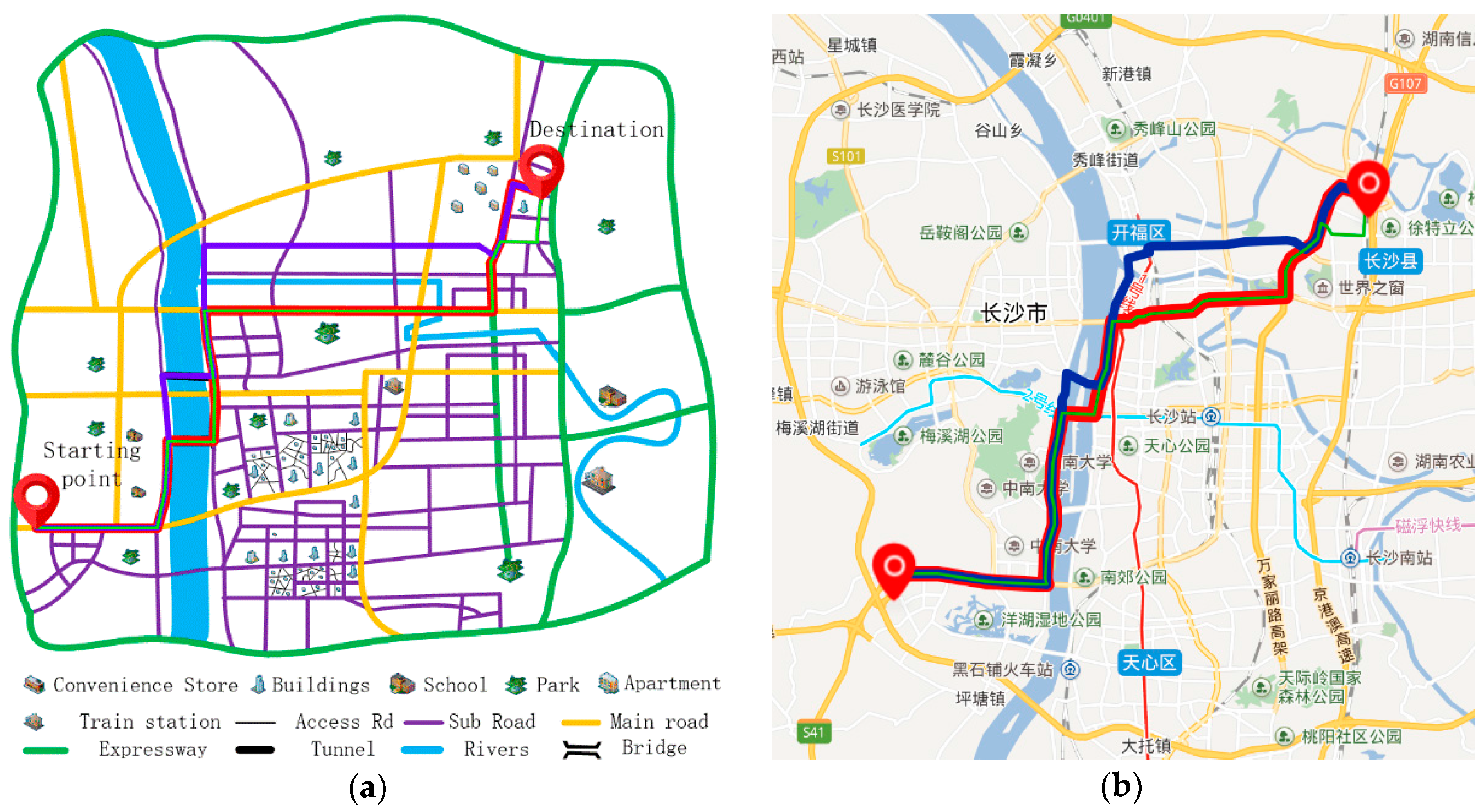
The optimal path model and actual planning path for user A are shown in Figure 9a,b, respectively. In these figures, blue denotes the optimal planning path for users of the same type [20], red denotes the optimal path to merge user A’s driving habits, and green denotes the log track of user A.

Figure 9 shows that in the landscape area, the blue and red paths are dominated by the surrounding landscape of Juzizhou Road, which showcases fresh air, beautiful scenery and low noise. The blue line represents the Yingpan road tunnel, and the red path shows the Orange Island Bridge across the area, overlooking the Orange Island scenery. The latter is in line with user A’s comfort requirements. In addition, the red route chooses the path from the perspective of user A, considering the comfort factors, and at the same time, it also focuses on the economic factors. In the non-sightseeing section, a small number of branches are allowed to reduce the detour distance to make up for the additional economic losses caused by the bypass of the two ends of the Orange Island Bridge. According to Table 11, the economic and comfort performance of the road and the effective length calculation indicate that the cumulative comfort consumption rates of the red planning path and blue reference path are 56.62 and 59.06, respectively, and the total economic losses are 88.28 and 88.19, respectively. In comparison with the reference path, the user personalization path that integrates user A’s habits increases comfort performance while decreasing economic performance slightly. The comfort performance increment of user A is contrary to the economic performance increment, and comparing the performance of the red and blue paths is difficult.

Hence, in this work, the increase in comfort loss is $\Delta C_{\mathrm{c}}=-2.44$, economic loss increment is $\Delta C_{\mathrm{m}}=0.09$ and is dimensionless, as shown in Formula (20). Between $c_{\mathrm{total}}$ and $m_{\mathrm{total}}$, t represents the time consumption of the red path and the total amount of economic consumption.

$$\{\begin{array}{l}\Delta C_{\mathrm{c}}^{\prime }=\frac{\left|\Delta C_{\mathrm{c}}\right|}{c_{\mathrm{total}}}\\ \Delta C_{\mathrm{m}}^{\prime }=\frac{\left|\Delta C_{\mathrm{m}}\right|}{m_{\mathrm{total}}}\end{array}$$

(20)

The calculation shows that $\Delta C_{\mathrm{c}}^{\prime }$ and $\Delta C_{\mathrm{m}}^{\prime }$ are satisfied in Formula (21).

$$\frac{\Delta C_{\mathrm{m}}^{\prime }}{0.32}<\frac{\Delta C_{\mathrm{c}}^{\prime }}{0.63}$$

(21)

Therefore, for user A, the increased comfort performance of the red path is greater than the economic performance reduction, the red path is more consistent with user A’s driving habits.

(2)

Example 2

Time + economic user B ([0.35,0.57,0.08]) and user A ([0.05,0.32,0.63]) show significant differences in driving characteristics. Specifically, the former places high importance in time and economic factors while ignoring the influence of comfort; that is, for time level 2, the influence coefficient is 0.35, and for time level 1, the influence coefficient is 0.57.

Reference example A makes personalized path planning from user B’s perspective, and the path planning process is no longer duplicated. The individual performance and effective length of the related roads are shown in

Table 12. Personalized performance of road based on B.

Path Name	Related Road	Level	T	M	C	Personal-Value	Effective Length/km
Individualization Route based on B	Yun Qi Road	4	0.49	0.35	0.53	0.37	3.77
	South Second Ring	4	0.49	0.35	0.53	0.37	8.77
	Labor East Road	5	0.35	0.30	0.39	0.29	1.37
	Wan Jiali viaduct	2	0.67	0.65	0.59	0.61	11.36
	Wanjiali North Road	6	0.37	0.32	0.47	0.31	2.54
	Xianghu West Road	7	0.28	0.30	0.34	0.27	1.13
Literature Reference Route	Yun Qi Road	4	0.49	0.35	0.53	0.45	3.77
	South Second Ring	4	0.49	0.35	0.53	0.40	8.77
	East Second Ring Road	3	0.37	0.22	0.38	0.25	8.78
	31 Avenue	3	0.48	0.28	0.43	0.33	1.95
	Wan Jiali viaduct	2	0.67	0.65	0.59	0.58	2.50
	Wan JialiNorth Road	6	0.37	0.32	0.47	0.31	2.54
	Xianghu West Road	7	0.28	0.30	0.34	0.27	1.13
Log trajectory	just as same as the personalized path that combines B’s habits

. Table 11 shows that the Yun Qi Road, South Second Ring, Wan Jiali viaduct, Wanjiali North Road, and Xianghu West Road appear in the path planning of users A and B; however, the road presents a considerable difference in terms of the personalized performance value and its effective length. Hence, verifying the performance of the proposed personalized path varies from person to person.

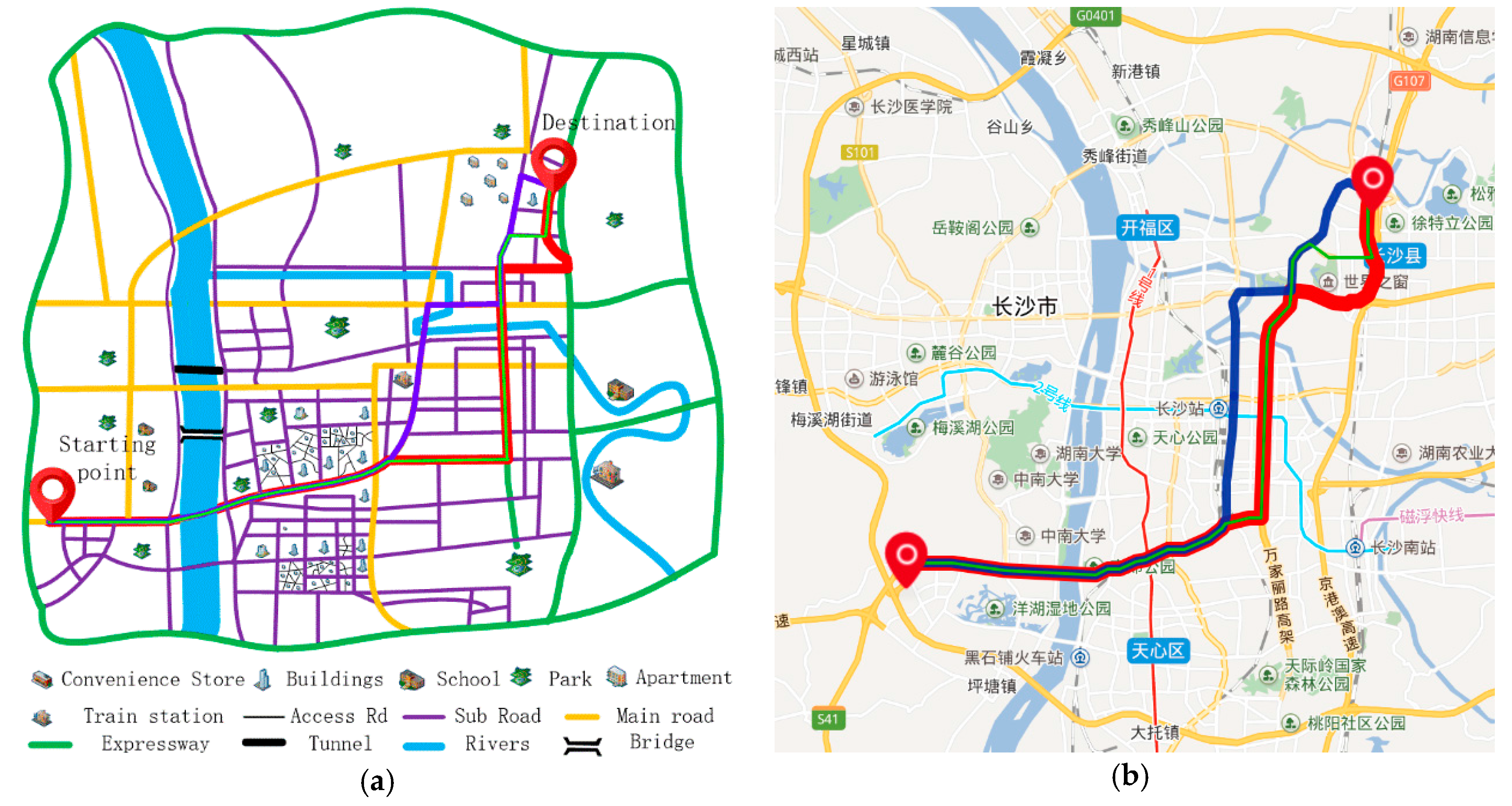
The optimal path model based on user B and the actual path, as shown in Figure 10a,b, respectively, remain unchanged in terms of the descriptions of the colors corresponding to the planning paths.

Figure 10 shows that the blue and red paths are driven mainly by the main road or viaduct, and they shorten the detour distance as much as possible. In comparison with the blue reference path, the red path representing the personalized path of user A can effectively avoid the East Second Ring Road, Bayi Road, South Road, Furong Road, Wuyi Road, and the bottleneck of a congested road. The road is relatively unimpeded. Moreover, by replacing Wan Jiali viaduct with going around the city at high speed, guaranteeing the time performance, it avoids the extra cost of passing through the road and the distance from the bypass, and improves the economic performance of the path.

According to the calculation results related to the time and economic performance and the effective road length in Table 12, the time consumption rates of the red planning path and blue reference path are 57.362 and 68.016, respectively, and the economic losses are 69.576 and 98.252, respectively. In comparison with the reference path, the personalized path that integrates user A’s habits shows improved comfort and economic performance. This result is consistent with the driving characteristics of user A, focusing on time and economic performance.

• Intra-class validation

(3)

Example 3

This example is the personalized path planning for time + economic user C ([0.56,0.37,0.07]), and user B’s planning path constitutes the intra-class verification of personalized path performance. Users C and B ([0.35,0.57,0.08]) share similar features, belong to the same time + economic type, pay attention to time and economic factors, while ignore the factors of comfort effect. However, there are two different levels of attention in time and economy. C users are more inclined to time, with a level of 1, a coefficient of 0.56, a second economic factor, a level of 2, and a coefficient of 0.37.

Reference example A makes personalized path planning from user C’s perspective. The personalized performance and effective length of the related roads are shown in

Table 13. Personalized performance of road based on C.

Route Type	Related Road	Level	T	M	C	Personal-Value	Effective Length/km
Individualization Route based on C	Yun-Qi Road	4	0.49	0.35	0.53	0.40	3.77
	South Second Ring	4	0.49	0.35	0.53	0.40	8.77
	Labor East Road	5	0.35	0.20	0.39	0.27	1.37
	Wan Jiali	2	0.67	0.65	0.59	0.62	8.82
	31 Avenue	3	0.48	0.28	0.43	0.37	2.17
	Xi Xia Road	6	0.49	0.36	0.47	0.41	4.93
literature Reference Route	Yun Qi Road	4	0.49	0.35	0.53	0.45	3.77
	South Second Ring	4	0.49	0.35	0.53	0.40	8.77
	East Second Ring Road	3	0.37	0.22	0.38	0.29	8.78
	31 Avenue	3	0.48	0.28	0.43	0.37	1.95
	Wan Jiali viaduct	2	0.67	0.65	0.59	0.58	2.50
	Wan jiali North	6	0.37	0.32	0.47	0.33	2.54
	Xianghu West Road	7	0.28	0.30	0.34	0.27	1.13
log trajectory	Yun Qi Road	4	0.49	0.35	0.53	0.40	3.77
	South Second Ring	4	0.49	0.35	0.53	0.40	8.77
	Labor East Road	3	0.35	0.20	0.39	0.27	1.37
	Wan Jiali viaduct	2	0.67	0.65	0.59	0.58	10.94
	Fuyuan East Road	6	0.45	0.35	0.41	0.38	1.22
	Kaiyuan West Road	6	0.45	0.35	0.41	0.38	1.29
	Xi Xia Road	6	0.49	0.36	0.47	0.41	2.60

.

Table 12 shows that the Yun Qi Road, South Second Ring, Wan Jiali viaduct, Wanjiali North Road, and Xianghu West Road also appear in the same type of path planning of users B and C. Path planning is of different types for users A and B. The same type of road users has different personalized performance, particularly for users B and C. With large effective length differences, the amplitude becomes increasingly small. The similarity obviously improves path planning. Path planning at a similar degree increases with the increase of similarity between user feature vectors.

The optimal path model based on user C’s driving habits and the actual planning path, as shown in Figure 11a,b, remain unchanged in terms of the descriptions of the colors corresponding to the planning paths.

By comparing Figure 10 and Figure 11, we can completely see that the blue reference path for user C in Figure 11 is consistent with that of user B in Figure 10, while the red planning path for user C in Figure 11 is only consistent with that of user B in Figure 10 at the beginning of the path planning, which avoids the East Second Ring Road and other regional centers and makes full use of time and economic advantages of Wanjiali viaduct; moreover, the inconsistent section steers clear of the Xianghu Road in densely populated areas, replacing it with Xi Xia Road that exhibits pedestrian sparsity, small confluence vehicles, and less traffic. According to the calculation results of time and economic performance and the effective road length shown in Table 13, the cumulative time consumption rates of the red planning path and blue reference path are 57.25 and 68.02, respectively, and the total economic losses are 77.69 and 98.25, respectively. In comparison with the reference path, the personalized path of user A shows significantly improved time and economic performance, as shown in

Table 14. Inter class contrast experiment.

Comparison Object	$\mathbf{\Delta }{\mathit{C}}_{\mathbf{t}}$	$\mathbf{\Delta }{\mathit{C}}_{\mathbf{m}}$	$\mathbf{\Delta }{\mathit{C}}_{\mathbf{t}}^{\mathbf{\prime }}$	$\mathbf{\Delta }{\mathit{C}}_{\mathbf{m}}^{\mathbf{\prime }}$	Result
Bibliographic reference path	−10.76	−20.56	—	—	Time performance ↑ Econommic performance ↑
Personalization path of fusion Based on B’s habits	−0.11	8.11	−0.002	0.104	$\frac{\Delta C_{\mathrm{t}}^{\prime }}{0.56}$ < $\frac{\Delta C_{\mathrm{m}}^{\prime }}{0.37}$

.

To embody the private custom advantage of the personalized planning path proposed in this paper, the user C is used as the specific service object in this verification link, except for the example of the reference path (blue in Figure 11b) experiments, adding the same type of personalized path (red in Figure 10b) contrast link.

Obviously, the contrast experiment on the personalized planning path that integrates user B’s habits does not meet the increment in time and economic consumption. Therefore, for the performance qualitative comparison link of Example 1, the dimensionless and performance comparison results are shown in Table 14.

Table 14 shows that in comparison with the reference path, the personalized planning path of user C shows greatly improved time and economic performance. This result is in line with the characteristics of the user related to time + economic performance. In comparison with the individual path planning of user B, the personalized path of user C shows improved time and economic performance; however, the benefits outweigh the lack of economic performance. This result is in line with user C’s greater attention time than economic performance levels.

• Calculation of degree of anastomosis

To establish the evaluation criteria for different planning paths and evaluate the performance of planning paths under different algorithms quantitatively, we introduce the path coincidence rate to characterize the matching degree between personalized paths. User driving habits Λ are satisfied in Formula (22).

$$\Lambda =\frac{l_{\mathrm{same}}}{l_{\mathrm{total}}}$$

(22)

Type $l_{\mathrm{same}}$ is the path length for the coincidence of planning path and log trajectory, $l_{\mathrm{total}}$ is the planning path length, and $l_{\mathrm{same}}$ ≤ $l_{\mathrm{total}}$. The results of the above example are listed as follows: comfort + economic user A, time + economic user B, time + economic user C personalized path/literature reference path and user log trajectory matching the result shown in

Table 15. Verification of path anastomosis.

Customer Type	Path Type	lsame/km	ltotal/km	Λ/a.u.
A	Bibliographic reference path	15.69	30.01	52.3%
	Personalization path based on A’s habits	26.77	30.01	89.2%
B	Bibliographic reference path	18.71	28.94	64.7%
	Personalization path based on B’s habits	28.94	28.94	100%
C	Bibliographic reference path	14.59	29.96	48.7%
	Personalization path based on C’s habits	25.33	29.96	84.5%

.

From Table 15, the coincidence degree levels of the personalized planning paths that integrates users A, B, and C are 89.2%, 100%, and 84.5%, respectively, which are different from the corresponding user log paths. The coincidence degrees of the planning paths are 52.3%, 64.7%, and 48.7%. In comparison with the reference path in the literature, the coincidence rate of the personalized path that integrates user habits and users’ log trajectory significantly increases by 36.9%, 35.3%, and 35.8%.

4. Conclusions

We propose a personalized path decision algorithm that is based on user habits, implementing the navigation service from a previous similar trip group to a specific individual, which can essentially improve the personalization of the existing path planning algorithms. the results and shortcomings of the existing optimization algorithms based on a single optimization target or a single or a few special traffic factors are analyzed. We use the log road track that integrates user’s habits to mine driving characteristics, and use LFCM to achieve user’s driving style clustering, and get users’ driving habits. Then, we use T-S based road multi index performance synchronous evaluation model to quantify the road’s time, economy and comfort performance. At the same time, we combine user’s driving style and feature to get the user’s road performance. Finally, ant colony algorithm is used to search the shortest path consumption path. The algorithm is based on the user’s own log trajectory and uses feature mining and clustering techniques to get the user’s habits and implements the navigated service objects from the previous travel groups to the travel individual and customizes personalized path navigation system for users to meet their own driving habits. The experimental results show that the absolute anastomosis rate and the relative anastomosis rate of the method in the simulated traffic network are 82% and 100%, respectively. In the actual traffic environment, three comparative examples (i.e., A, B, and C) of user’s personalized path and the corresponding user log path show consistent rates, reaching 89.2%, 100%, and 84.5%, respectively; in comparison with the individual path in the literature [20], the path coincidence rate significantly increases by 36.9%, 35.3%, and 35.8%, respectively. By improving the personalization level of existing path planning, the travel experience of self-driving users is greatly improved.

References

- Ma, J.; Sun, G. Mutation Ant Colony Algorithm of Milk-Run Vehicle Routing Problem with Fastest Completion Time Based on Dynamic Optimization. Discret. Dyn. Nat. Soc. 2013, 2013, 418436. [Google Scholar] [CrossRef]
- Guo, J.; Wu, Y.; Zhang, X.; Zhang, L.; Chen, W.; Cao, Z.; Zhang, L.; Guo, H. Finding the ‘faster’ path in vehicle routing. IET Intell. Transp. Syst. 2017, 11, 685–694. [Google Scholar] [CrossRef]
- Tang, K.; Qian, M.; Duan, L. Choosing the fastest route for urban distribution based on big data of vehicle travel time. In Proceedings of the International Conference on Service Systems and Service Management, Dalian, China, 16–18 June 2017; pp. 1–4. [Google Scholar]
- Li, Z.; Kolmanovsky, I.V.; Atkins, E.M.; Lu, J.; Filev, D.P.; Bai, Y. Road Disturbance Estimation and Cloud-Aided Comfort-Based Route Planning. IEEE Trans. Cybern. 2016, 47, 3879–3891. [Google Scholar] [CrossRef] [PubMed]
- Faizian, P.; Mollah, M.A.; Yuan, X.; Pakin, S.; Lang, M. Random Regular Graph and Generalized De Bruijn Graph with k-shortest Path Routing. IEEE Trans. Parallel Distrib. Syst. 2018, 29, 144–155. [Google Scholar] [CrossRef]
- Idri, A.; Oukarfi, M.; Boulmakoul, A.; Zeitouni, K.; Marsi, A. A distributed approach for shortest path algorithm in dynamic multimodal transportation networks. Trans. Res. Procedia 2018. [Google Scholar] [CrossRef]
- Zhang, Y.; Song, S.; Shen, Z.J.M.; Wu, C. Robust Shortest Path Problem with Distributional Uncertainty. IEEE Trans. Intell. Transp. Syst. 2017. [Google Scholar] [CrossRef]
- Zhang, D.; Yang, D.; Wang, Y.; Tan, K.-L.; Cao, J.; Shen, H.T. Distributed shortest path query processing on dynamic road networks. VLDB J. 2017, 26, 399–419. [Google Scholar] [CrossRef]
- Mark, T.; Griffin, M.J. Motion sickness in public road transport: The effect of driver, route and vehicle. Ergonomics 1999, 42, 1646–1664. [Google Scholar]
- Yao, Y.; Peng, Z.; Xiao, B.; Guan, J. An efficient learning-based approach to multi-objective route planning in a smart city. In Proceedings of the IEEE International Conference on Communications, Paris, France, 21–25 May 2017. [Google Scholar]
- Siddiqi, U.F.; Shiraishi, Y.; Sait, S.M. Multi-objective optimal path selection in electric vehicles. Artif. Life Robot. 2012, 17, 113–122. [Google Scholar] [CrossRef]
- Ahmed, F.; Deb, K. Multi-objective optimal path planning using elitist non-dominated sorting genetic algorithms. Soft Comput. 2013, 17, 1283–1299. [Google Scholar] [CrossRef]
- Bazgan, C.; Jamain, F.; Vanderpooten, D. Approximate Pareto sets of minimal size for multi-objective optimization problems. Oper. Res. Lett. 2015, 43, 1–6. [Google Scholar] [CrossRef]
- Kriegel, H.P.; Renz, M.; Schubert, M. Route skyline queries: A multi-preference path planning approach. In Proceedings of the IEEE International Conference on Data Engineering, Long Beach, CA, USA, 1–6 March 2010; pp. 261–272. [Google Scholar]
- Song, X.; Cao, H.; Huang, J. Influencing Factors Research on Vehicle Path Planning Based on Elastic Bands for Collision Avoidance. SAE Int. J. Passeng. Cars Electron. Electr. Syst. 2012, 5, 625–637. [Google Scholar] [CrossRef]
- Yook, D.; Heaslip, K. The effect of crowding on public transit user travel behavior in a large-scale public transportation system through modeling daily variations. Transp. Plan. Technol. 2015, 38, 935–953. [Google Scholar] [CrossRef]
- Feng, P. The Research of Dynamic Path Planning Based on Improving Fuzzy Genetic Algorithm in the Vehicle Navigation. Adv. Mater. Res. 2012, 424–425, 73–76. [Google Scholar] [CrossRef]
- Jiang, H.; Yuan, R.; Wang, T.; Wang, R. Research on Green Path Planning Model for Road Logistics Vehicle. In Proceedings of the International Conference of Logistics Engineering and Management, Chengdu, China, 8–10 October 2010; pp. 3082–3088. [Google Scholar]
- Chen, Z.; Shen, H.T.; Zhou, X. Discovering popular routes from trajectories. In Proceedings of the IEEE, International Conference on Data Engineering, Hannover, Germany, 11–16 April 2011; IEEE Computer Society: Washington, DC, USA, 2011; pp. 900–911. [Google Scholar]
- Campigotto, P.; Rudloff, C.; Leodolter, M.; Bauer, D. Personalized and Situation-Aware Multimodal Route Recommendations: The FAVOUR Algorithm. IEEE Trans. Intell. Transp. Syst. 2017, 18, 92–102. [Google Scholar] [CrossRef]
- Nadi, S.; Houshyaripour, A.H.; Nadi, S.; Houshyaripour, A.H. A new model for fuzzy personalized route planning using fuzzy linguistic preference relation. Int. Arch. Photogramm. Remote Sens. Spatial Inf. Sci. 2017, XLII-4/W4, 417–421. [Google Scholar] [CrossRef]
- Dai, J.; Yang, B.; Guo, C.; Ding, Z. Personalized route recommendation using big trajectory data. In Proceedings of the IEEE International Conference on Data Engineering, Seoul, Korea, 13–17 April 2015; pp. 543–554. [Google Scholar]
- Letchner, J.; Krumm, J.; Horvitz, E. Trip router with individualized preferences (TRIP): Incorporating personalization into route planning. In Proceedings of the National Conference on Artificial Intelligence and the Eighteenth Innovative Applications of Artificial Intelligence Conference, Boston, MA, USA, 16–20 July 2006; pp. 1795–1800. [Google Scholar]
- Zhu, X.; Hao, R.; Chi, H.; Du, X. FineRoute: Personalized and Time-Aware Route Recommendation Based on Check-ins. IEEE Trans. Veh. Technol. 2017, 66, 10461–10469. [Google Scholar] [CrossRef]
- Long, Q.; Zeng, G.; Zhang, J.; Zhang, L. Dynamic route guidance method for driver’s individualized demand. J. Cent. South Univ. (Nat. Sci. Ed.) 2013, 44, 2124–2129. [Google Scholar]
- Ness, M.; Herbert, M. A prototype low cost in-vehicle navigation system. In Proceedings of the 1993 Vehicle Navigation and Information Systems Conference, Ottawa, ON, Canada, 12–15 October 1993; pp. 56–59. [Google Scholar]
- Tang, T.Q.; Xu, K.W.; Yang, S.C.; Shang, H.Y. Analysis of the traditional vehicle’s running cost and the electric vehicle’s running cost under car-following model. Mod. Phys. Lett. B 2016, 30, 1650084. [Google Scholar] [CrossRef]
- Kapoor, A.; Singhal, A. A comparative study of K-Means, K-Means++ and Fuzzy C-Means clustering algorithms. In Proceedings of the International Conference on Computational Intelligence & Communication Technology, Ghaziabad, India, 9–10 February 2017; pp. 1–6. [Google Scholar]
- Balteanu, A.; Jossé, G.; Schubert, M. Mining Driving Preferences in Multi-cost Networks. In Proceedings of the International Conference on Advances in Spatial and Temporal Databases, Munich, Germany, 21–23 August 2013; Springer: New York, NY, USA, 2013; pp. 74–91. [Google Scholar]
- Zhou, L.; Tong, L.; Chen, J.; Tang, J.; Zhou, X. Joint optimization of high-speed train timetables and speed profiles: A unified modeling approach using space-time-speed grid networks. Transp. Res. Part B Methodol. 2017, 97, 157–181. [Google Scholar] [CrossRef]
- Yang, M.S.; Nataliani, Y. Robust-learning fuzzy c-means clustering algorithm with unknown number of clusters. Pattern Recognit. 2017, 71, 45–59. [Google Scholar] [CrossRef]
- Wang, Q.; Zhang, Y.; Xiao, Y.; Li, J. Kernel-based fuzzy C-means clustering based on fruit fly optimization algorithm. In Proceedings of the 2017 International Conference on Grey Systems and Intelligent Services, Stockholm, Sweden, 8–11 August 2017; pp. 251–256. [Google Scholar]
- Taha, A.A.; Hanbury, A. An Efficient Algorithm for Calculating the Exact Hausdorff Distance. IEEE Trans. Pattern Anal. Mach. Intell. 2015, 37, 2153–2163. [Google Scholar] [CrossRef] [PubMed]
- Chen, Y.; He, F.; Wu, Y.; Hou, N. A local start search algorithm to compute exact Hausdorff Distance for arbitrary point sets. Pattern Recogn. 2017, 67, 139–148. [Google Scholar] [CrossRef]
- Ji, P.; Zhang, H.Y. A subsethood measure with the hausdorff distance for interval neutrosophic sets and its relations with similarity and entropy measures. In Proceedings of the Control and Decision Conference, Yinchuan, China, 28–30 May 2016; pp. 4152–4157. [Google Scholar]
- Li, T.; Pan, Q.; Gao, L.; Li, P. A novel simplification method of point cloud with directed Hausdorff distance. In Proceedings of the IEEE, International Conference on Computer Supported Cooperative Work in Design, Wellington, New Zealand, 26–28 April 2017; pp. 469–474. [Google Scholar]
- Department of People’s Republic of China Construction Department. Urban Road Traffic Planning and Design Specification; China Planning Press: Beijing, China, 1995.
- Ren, F. Road Capacity Manual: Special Report of the United States Traffic Research Committee No. 209; China Construction Industry Press: Beijing, China, 1991. [Google Scholar]
- Xiao, S.; Zhang, Y.; Zhang, B. Adaptive synchronization of delayed T-S type fuzzy neural networks. In Proceedings of the IEEE Control and Decision Conference, Qingdao, China, 23–25 May 2015; pp. 1726–1731. [Google Scholar]
- Li, P.F.; Ning, Y.W.; Jing, J.F. Research on the detection of fabric color difference based on T-S fuzzy neural network. Color Res. Appl. 2017, 42, 609–618. [Google Scholar] [CrossRef]
- Wei, X.; Chang, X.Q. The Optimization Design of Emergency Logistics Distribution Path Based on Ant Colony Algorithm. In Proceedings of the 6th International Asia Conference on Industrial Engineering and Management Innovation; Atlantis Press: Amsterdam, The Netherlands, 2016. [Google Scholar]
- Yang, Q.; Chen, W.N.; Yu, Z.; Gu, T.; Li, Y.; Zhang, H.; Zhang, J. Adaptive Multimodal Continuous Ant Colony Optimization. IEEE Trans. Evol. Comput. 2017, 21, 191–205. [Google Scholar] [CrossRef]
- Wang, R.; Zheng, D.; Zhang, H.; Mao, J.; Guo, N. A solution for simultaneous adaptive ant colony algorithm to memory demand vehicle routing problem with pickups. In Proceedings of the Control and Decision Conference, Yinchuan, China, 28–30 May 2016; pp. 2172–2176. [Google Scholar]
- Liu, Z.; Jiang, J.; Yang, Y.; Wang, S. Adaptive ant colony algorithm based on cloud model. In Proceedings of the IEEE International Conference on Information and Automation, Lijiang, China, 8–10 August 2015; pp. 2654–2657. [Google Scholar]
Figure 1.
The log fuzzy C-means algorithm (LFCM) algorithm.
Figure 2.
Vehicle space–time path.
Figure 3.
The result of LFCM.
Figure 4.
(a) Initialize the valid range of the sample; (b) The corresponding plane projection of the initialization process; (c) Determining the effective radius of clustering; (d) The corresponding plane projection of the effective radius of clustering; (e) Effective sample screening results; (f) The corresponding plane projection of the result of Effective sample screening process.
Figure 5.
Performance synchronization evaluation model of road multidimensional standard.
Figure 6.
Improved adaptive ant colony algorithm and its contribution.
Figure 7.
Analog road network.
Figure 8.
Comparison of simulation effect.
Figure 9.
(a) The optimal path model for user A; (b) The optimal actual planning path for user A. Where, the green represents log trajectory, the blue represents literature Reference resources Route, and the red represents the Individualization Route based on A. Detailed performance of the relevant roads refer to Table 11.
Figure 10.
(a) The optimal path model for user B; (b) The optimal actual planning path for user B. Where, the green represents log trajectory, the blue represents literature Reference resources Route, and the red represents the Individualization Route based on B. Detailed performance of the relevant roads refer to Table 12.
Figure 11.
(a) The optimal path model for user C; (b) The optimal actual planning path for user C. Where, the green represents log trajectory, the blue represents literature Reference resources Route, and the red represents the Individualization Route based on B. Detailed performance of the relevant roads refer to Table 13.