Depth Retrieval Procedures in Pulsed Thermography: Remarks in Time and Frequency Domain Analyses

Featured Application

The present study intends to show the potentiality of pulsed thermographic imaging to quantitatively characterise hidden defects in Carbon Fibre Reinforced Polymers. By comparing the performance of different depth retrieval procedures, it was possible to evaluate the produced depth estimation accuracy and to define the impact of different experimental and analysis parameters in quantitative analysis.

Abstract

In the present study, a Carbon Fibre Reinforced Polymer (CFRP) sample of trapezoid shape, consisting of internal artificial delaminations of various sizes and depth locations, is investigated by means of optical pulsed thermography for the retrieval of quantitative depth information. The main objectives of this work are to evaluate the produced depth estimation accuracy from two contrast-based depth inversion procedures as well as to correlate the acquired results with characteristics such as the location and size of the detected features and with analysis parameters such as the selection of the sound area. Quantitative analysis is performed in both the temporal and frequency domains, utilising, respectively, the informative parameters of thermal contrast peak slope time and blind frequency. The two depth retrieval procedures are applied for the depth estimation of features ranging in size from 3 mm to 15 mm and in depth from 0.2 mm to 1 mm. The results of the present study showed that the two different analyses provided efficient depth estimations, with frequency domain analysis presenting a greater accuracy. Nevertheless, predicting errors were observed in both cases and the factors responsible for these errors are defined and discussed.

1. Introduction

Pulsed Thermography (PT) is a widely used technique for the Non-Destructive Testing and Evaluation (NDT&E) of advanced materials and structures [1,2,3,4,5]. Compared with other NDT&E technologies, this thermographic configuration presents remarkable benefits such as its rapid and simple implementation, its suitability for large-scale inspections and complex surface monitoring, as well as its contactless application requiring no physical contact to the material being inspected. The implementation of a pulsed thermographic inspection is based on the monitoring of the heat transfer occurred during the cooling of the test item after the application, usually to its surface, of an instantaneous and high energy pulse heating procedure [6]. The application of the thermal stimulus is followed by the recording of the resultant surface temperature response through the aid of an IR camera, aiming to detect changes in the surface temperature distribution. These changes are normally owned to the presence of internal defects and/or discontinuities which are altering the heat diffusion rate into the inspected component.

Nowadays, PT is recognised as a testing procedure that can provide inspectors not only with the ability to detect defects, but also the means to quantify these defects for continuous monitoring and assessment [7]. This is a result of the advances in thermographic imaging technology that have orientated the analysis to the independent spatial and/or temporal treatment of each pixel of the thermal images’ sequence, along with the development and use of advanced signal processing techniques [8,9]. Signal processing techniques have been developed for the interpretation of infrared thermographic data, targeting the defect detectability enhancement and noise reduction on the final imaging output, while the importance of these processing tools is also devoted to the preparation of data for the continuation to the phase of quantitative characterisation [10,11].

Regardless of the domain where the thermal data are processed (the most common are temporal domain processing and frequency domain processing), different techniques have been proposed to quantitatively characterise detected defects. These techniques are based either on analytical methods [12] or inverse methods that are implementing numerical calculations and experimental measurements [13]. In the former case, experimental data can somehow produce results in a straightforward manner, as these are used to solve analytical formulas. On the other hand, by involving inverse techniques, quantitative characterisation requires the establishment of a numerical model taking into account many parameters. Usually, only one parameter is of interest (e.g., depth) which can be estimated by correlating the numerical and the experimental results. Quantitative characterisation by means of pulsed, and more generally speaking of active thermal imaging, includes mainly depth information retrieval [14,15,16,17,18] and the estimation of defect’s lateral dimension [19,20,21], while several studies have also investigated the determination of the thermal properties either of the material being inspected [22,23] or of the hidden features [24].

Based on the above mentioned, the present study focused to the application of optical Pulsed Thermography for the quantitative characterisation of induced artificial defects in a CFRP component, aiming to highlight the strengths and limitations of this technique in similar quantitative inspections. The quantitative depth estimation procedures applied in this study evaluated the performance of two contrast-based methods, one in the time and one in the frequency domain, respectively, and in particular through the study of the temperature–contrast slope temporal variations and the monitoring of the phase-contrast variations as a frequency function. These analytical methods for depth prediction require the need for a sound area determination and thus a comparison was performed regarding the influence degree of the sound area selection in depth prediction accuracy working with either raw temperature or phase data. The depth results produced from the two quantification procedures were compared in terms of error production, and the divergences observed between the estimated and the pre- known nominal depths were evaluated taking into consideration the specifications of the investigated sample along with the experimental parameters selected to conduct this study. In the following, a brief description of the quantification techniques used in this study is presented.

1.1. Quantitative Depth Estimation in the Time Domain

For quantitative depth prediction in the time domain, the most widely used algorithms utilise temporal characteristics of the thermal response received from the tested surface. In particular, these methods are based on the correlation of the defect’s depth with a time point at which the hidden feature appears as a temperature difference on the surface of the inspected sample. The idea behind the determination of these time points is based on the fact that, when studying the heat diffusion into the material bulk after the application of a thermal pulse, the time taken for the thermal wave to be reflected back to the surface is inversely proportional to the thermal diffusivity of the material and directly proportional to the square of its depth [6]. The first proposed and the most commonly used method utilises the time point when the maximum thermal contrast between a defective and a preselected reference point occurs, known as Peak Contrast Time [25,26,27]. Even though this informative parameter can produce quantitative depth information, one of its major limitations is the fact that the peak contrast appears relatively late, when the 3D heat diffusion around the defect has a great influence on the acquired result. Consequently, different methods have also been proposed investigating the use of earlier temporal points, targeting to the produced accuracy enhancement.

One of the earliest time points on a temperature–time evolution curve, which is used for defect depth estimations, is the moment when the behaviour of the studied temperature signal above the defect diverges from the behaviour of the reference signal [28]. Usually, as raw thermal data contain noise, the establishment of a threshold level is required to identify this point on the temperature–time curve [29]. Quantitative depth estimations through the aid of this informative parameter have the advantage of early depth prediction, thus possible effects produced from lateral heat diffusion in the defective area are negligible. However, the determination of this value requires a sampling rate high enough to accurately capture the initial time when the temperature in the defective zone diverse from the reference temperature, impeding the providing of accurate results in the case of shallow defects characterisation [30].

A later time interval but early enough to suppress the negative effects of lateral heat diffusion is the moment when the thermal contrast curve presents its peak slope [31,32]. This point can be easily found as it corresponds to the peak of the 1st derivative of the thermal contrast and is commonly referred as Peak Slope Time method. The exact relationship between depth and peak slope time can be determined by solving, for this specific time value, Equation (1) [33]:

$$t_{peak}=\frac{3.64z^2}{{\pi }^2\alpha }$$

(1)

where t_peak is the time at which the peak in the slope contrast occurs, z is the defect depth in a sample of thickness L and α the thermal diffusivity of the tested material. This parameter is essential for defect depth estimation as experimental and numerical studies have shown that results are unaffected from the size of the defect, while the proportionality coefficient equal to 3.64 was found to be valid regardless the type of the material when $z/L\le 0.5$ [33].

1.2. Quantitative Depth Estimation in the Frequency Domain

Frequency domain analysis using quantitative Pulsed Phase Thermography (PPT) and phase data are of prime interest in thermographic imaging, as, in addition to the enhanced detectability that this technique provides, a depth prediction approach similar to the early detection in time domain analysis has been developed and widely used [34,35]. This approach consists of identifying the depth of the defect from the frequency for which the phase contrast between a defective and a sound area crosses the zero-contrast line. This technique relies on the thermal diffusion length, i.e., μ = (α/πf)^1/2 as the depth of the defect can be estimated from a relationship of the form [36]:

$$z=C·\mu =C\sqrt{\frac{\alpha }{\pi f_b}}$$

(2)

where C is a correlation constant and f_b (Hz) is the blind frequency, defined as the limiting frequency at which the feature of interest presents enough phase contrast for its detection in the frequency spectrum. The above described procedure for quantitative analysis requires the determination of the blind frequency and of the correlation coefficient C, when the material’s thermal properties are known. Conventional experimental C values when using the phase in lock-in experiments range from 1.5 to 2 [37] with a value of C = 1.82 typically adapted in experimental studies [38,39]. PPT results agree with this value range either for homogeneous or composite materials [35,36]. Thus, when the value of proportionality coefficient is known, the quantitative PPT requires the measurement of the blind frequency. In any other case, to validate the depth results, the accuracy of the correlation coefficient value used in Equation (2) should be graphically evaluated by the variables z and µ [36].

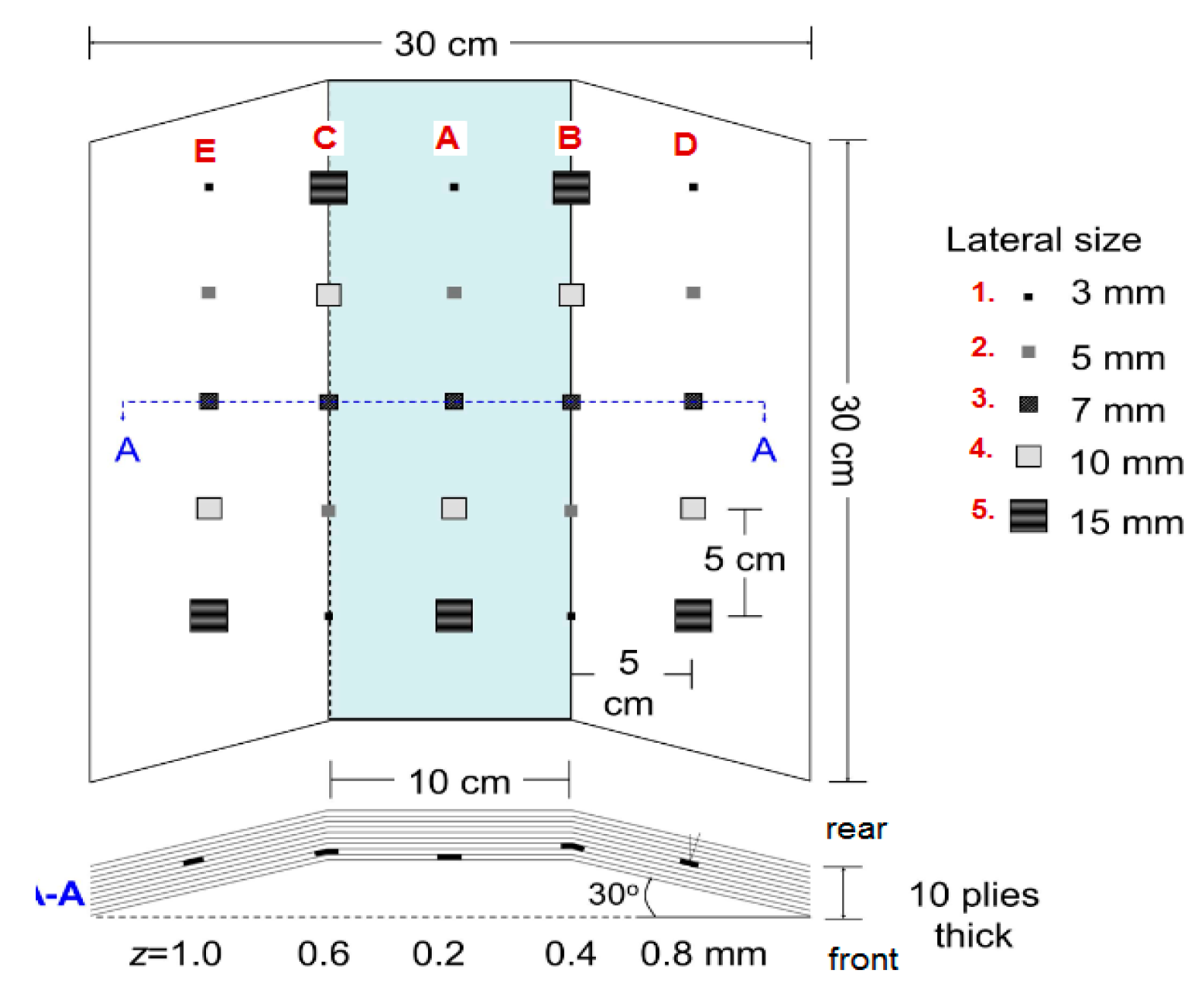
2. Materials and Methods

To evaluate the potential of pulsed thermography for quantitative depth characterisation, experimental testing was carried out in a trapezoid CFRP laminate, having fabricated defects of known characteristics. The CFRP sample was a laminate 30 cm × 30 cm trapezoid structure consisted of ten (10) plies giving a total specimen thickness of 2 mm and a laminae orientation of 0°/90° cross ply through its volume. As illustrated in the schematic of Figure 1, 25 square Teflon^TM insertions of different dimensions ranging from 3 mm to 15 mm were placed between the plies simulating local detached regions. These insertions were divided into five series (A–E in the schematic), placed at different depths ranging from 0.2 mm to 1 mm, while each series consisted of five square insertions of different lateral dimensions (No. 1 to No. 5 in the schematic). As stated above, the sample was inspected by depositing heat energy on its rear surface, the opposite from this presented in Figure 1, allowing a depths’ range investigation from 0.2 mm to 1 mm. The convenience of inspecting this component (widely used in several studies) is derived from the fact that its characteristics and the presence of similar defects at different depths enable the conduction of relative comparisons.

For data acquisition, a flash thermographic system in reflection mode was used and two high energy flash lamps were triggered at t = 0 s to deposit an instantaneous (of a 5 ms pulse duration) heat pulse on the sample’s surface. The temporal and spatial surface temperature variations after the application of the energy pulse were monitored through the aid of a high-speed infrared camera, capturing a sequence of thermal images during the cooling down phase. The camera used in this study was a mid-wave (3–5 µm) device, containing a focal plane array of 320 × 256 infrared detectors. The experimental parameters used to acquire the thermographic sequence along with the characteristics of the inspection equipment are summarised in

Table 1. Experimental equipment and acquisition parameters.

Experimental Equipment	Acquisition Parameters
Thermal stimulation: Photographic Flashes: Balcar FX 60 pulse duration: 5 ms thermal pulse, deposited energy: 3.2 KJ/ flash (total energy deposited 6.4 KJ) Thermographic monitoring: Santa Barbara infrared camera, Focal Plane Array, nitrogen cooled, InSb, 320 × 256 pixels	Sampling rate, ${\mathrm{f}}_{\mathrm{s}}$	157 Hz
	Acquisition duration, $t_{acq}$	6.7 s
	Time interval, $\Delta t=1/f_s$	6.3 ms
	Total number of frames, N	1052

.

The acquired pulsed thermal dataset measured the two dimensional surface temperature distribution T(x,y) as a function of time t. Because quantification in the frequency domain requires the application of PPT technique to treat the raw data, which is a pixel-wise transformation technique, and to increase the data processing speed, it should be noted that before continuing to the data analysis phase, the recorded data were sub-sampled by a factor of 4. As a result, the parameters of the truncated sequence were redefined as N = 263 frames, f = 39.25 Hz, and time interval Δt = 25 ms. The adoption of the above sub-sampling procedure had a dual objective, initially to overcome the long computation times and secondly to assess the impact degree of the sampling resolution to the acquisition of quantitative depth results. In such a manner and by capturing the data at the highest sampling rate of the apparatus, an inefficient resolution could be easily re-optimised through the selection of a lower sub-sampling factor and without the need of capturing a new dataset.

As stated above, the quantitative depth determination procedures applied in this study, evaluated the performance of two contrast-based methods. The correlation expressions used to determine the depth z of the inserts were based on the determination of the thermal contrast peak slope time (time domain analysis) and of the blind frequency (frequency domain analysis) using the Equations (1) and (2), respectively. As a result, for known thermal properties of the tested material, the determination of t_peak and f_b can be used for depth quantification purposes. Additionally, the correlation factor C used in this study (frequency domain analysis) had the value of 1.82, while the thermal diffusivity α of the inspected component according to its manufacturing characteristics was defined by the literature, having the value of 4.2 × 10⁻⁷ m² s⁻¹ [6].

Both the temporal and the frequency domain quantification techniques required the selection of a sound area. An inappropriate sound area selection can be an important factor for error production when depth has to be estimated, making its selection the most crucial parameter which in combination with a non-uniform stimulation process can provide large deviations from the actual depth in which the detected feature is located to. Based on the qualitative assessment of the examined sample presented in a previous study by the authors [40], which showed that temperature data elaboration suffered from uneven heating, depth quantification in the time domain was designed by selecting the sound area next to each defect. In such a manner, it was ensured that the two respective regions received the same amount of heat energy and consequently minimising errors due to uneven heating. In particular, according to the lateral dimensions of the detected Teflon squares, a sound area occupying exact the same pixels as the defective one was selected next to the insertion as illustrated in Figure 2 and their dimensions were defined in terms of pixels as 4 × 4, 6 × 6, 8 × 8, 10 × 10 and 12 × 12 for correspondent defects No. 1, No. 2, No. 3, No. 4 and No. 5.

However, as the application of PPT produced enhanced background uniformity, only an area from the background was selected for the calculations of the produced phase contrasts. In other words, contrary to the time domain analysis the same sound area was used in this case for the calculations of all the phase contrast curves and consequently for the depth measurements of the detected features. Additionally, due to the enhanced background uniformity observed on the frequency domain analysis, this depth quantification method was repeated and assessed, considering as well the field of view as the sound area. For the clarity of the readers about the above selections, indicative imaging results from the two domains are presented in Figure 3, justifying the decisions concerning the selection of the sound areas in both the temporal and frequency domain analysis. In particular, the influence of uneven heating can be observed in Figure 3a, contrary to the phase image of Figure 3b, where background uniformity was observed.

3. Results and Discussion

In the following, the results from the two quantification methods are presented and discussed. Initially, the two quantification procedures along with the informative parameters utilised in each case are evaluated followed by the presentation of the depth results in each case, while at the end of this section a comparison of temporal and frequency domain analysis in term of error production is reported.

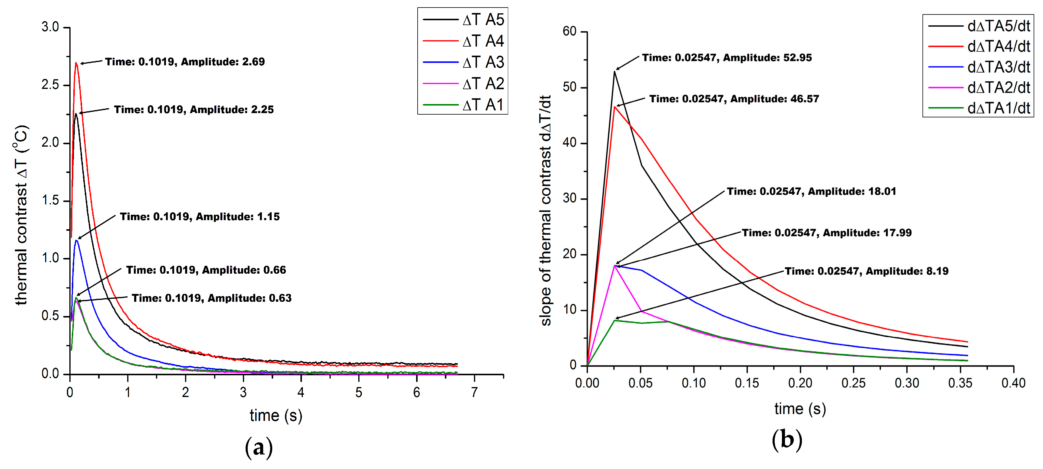
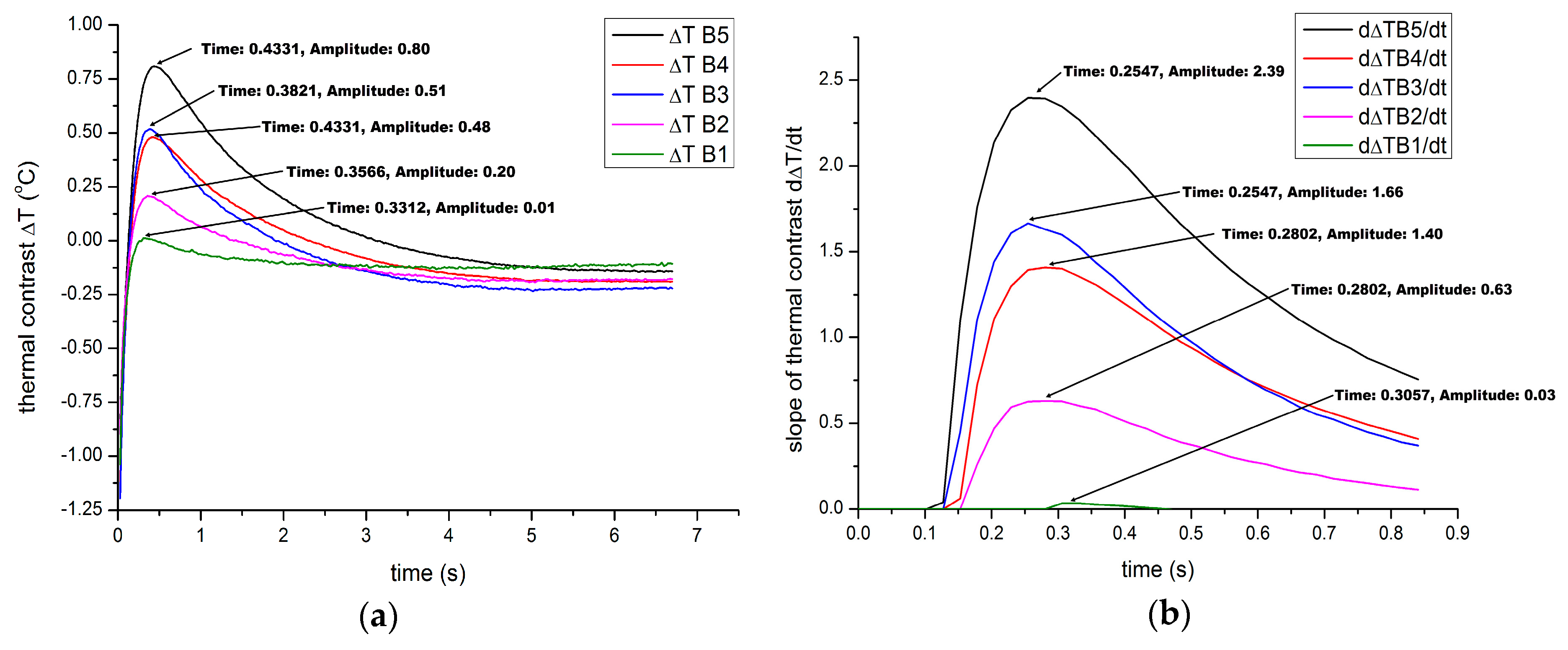
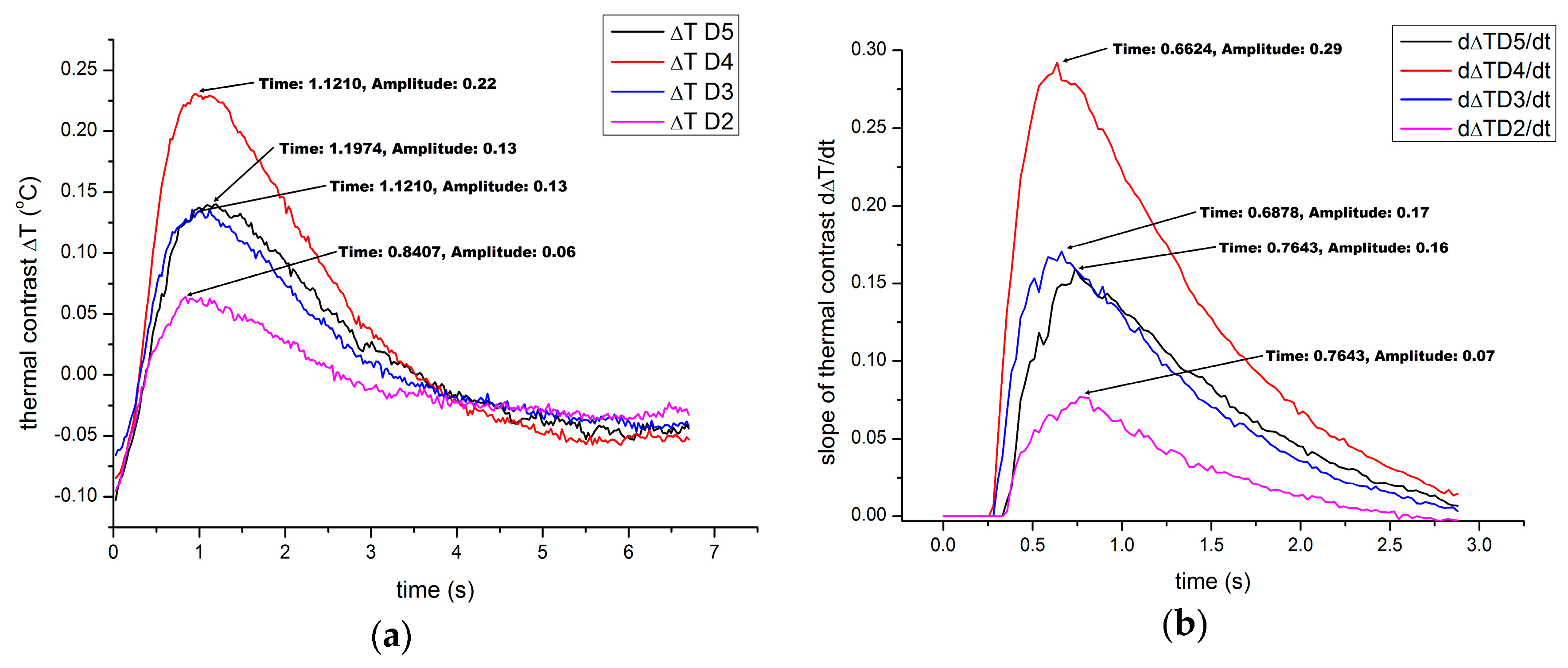
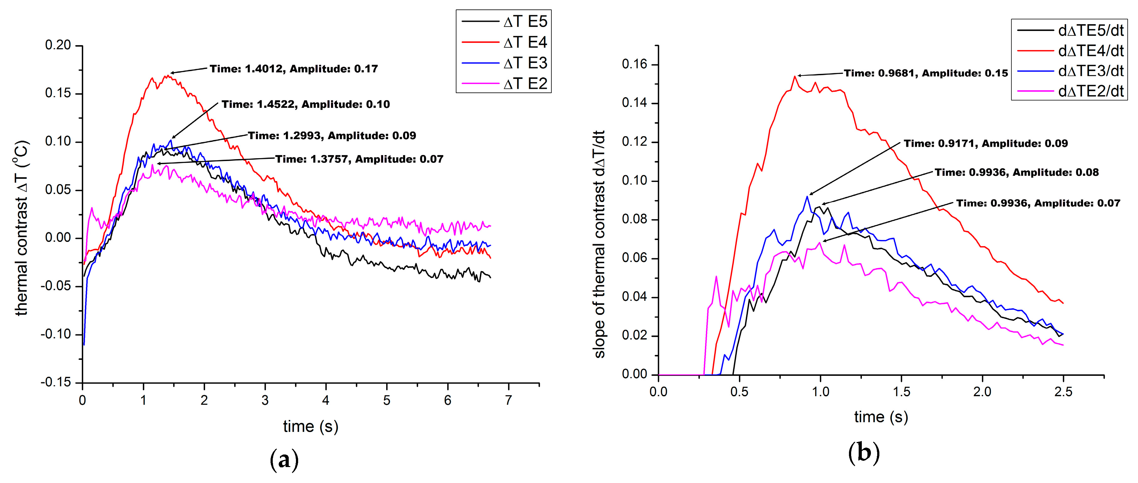
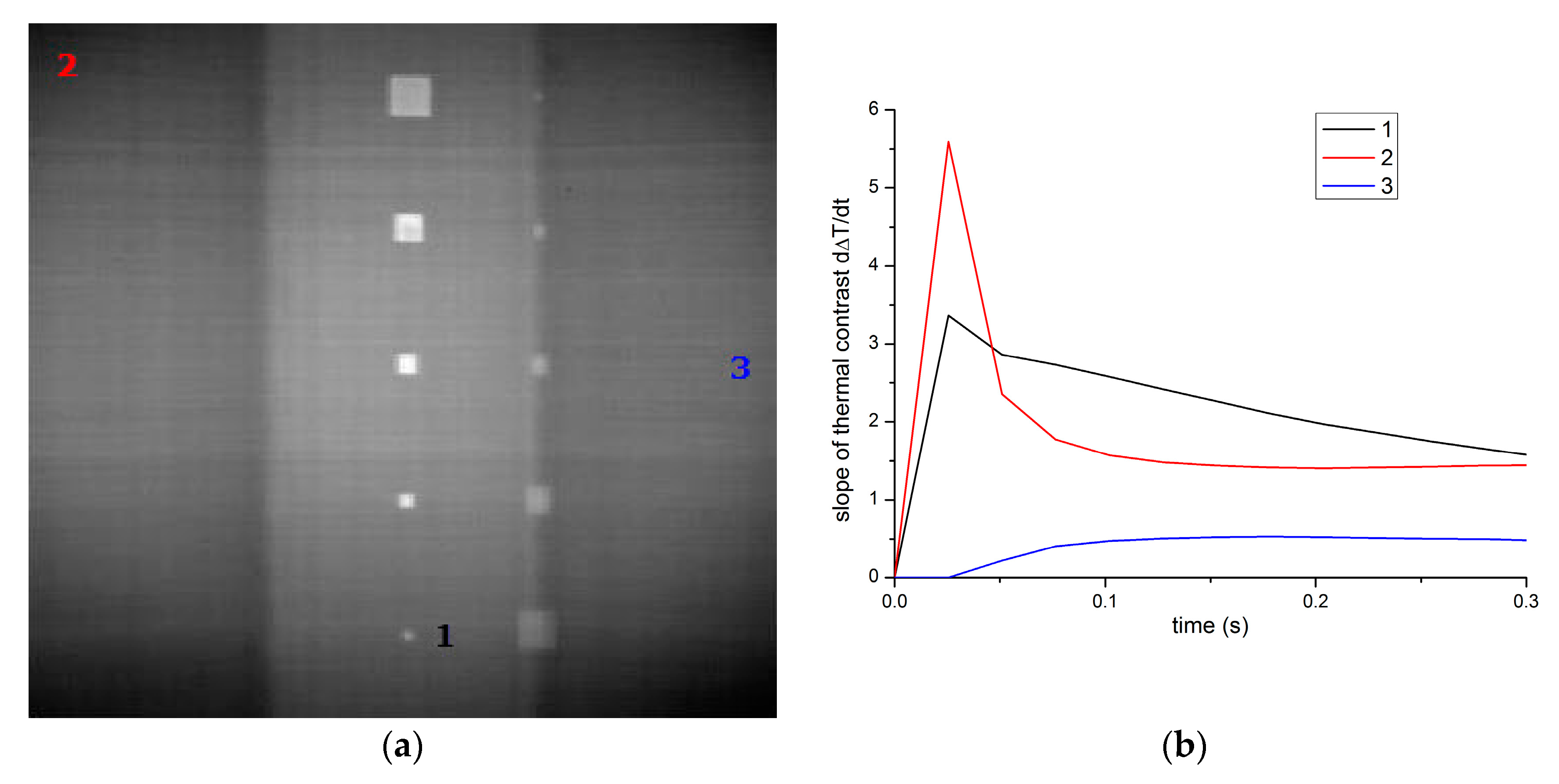
3.1. Depth Retrieval with Thermal-Contrast Peak Slope Time

After the application of the pulse thermal energy and the recording of the surface temperature response, the delaminated regions’ detection was produced due to the lower thermal conductivity that these features have with respect to the host material. The variation in the thermal properties affected the penetration rate of the heat flux into the composite bulk and therefore the surface temperature distribution, resulting to the appearance of local “hot spots”. The time points of these hot spots appearance were varied according to the inserts’ location (depth) and size. Thus, when raw temperature data are handled, the depth at which these inserts are located to, can be determined by subtracting the cooling curve over a reference area from the cooling curve over the damaged one. The resulting temperature difference curve can produce the correlation of the detected feature’s depth with two characteristic points, this of peak temperature difference and this of the peak slope of this difference, which are further associated with the correspondent times when these phenomena occur (peak contrast time and peak slope time).

Before the actual depth information retrieval through the correlation of these specific time points with the depth of the detected features, the temporal functions of the thermal contrast and of the slope of this contrast were studied, verifying that the selection of peak slope time for depth calculations is a more appropriate method, when working with raw temperature data. The experimental results in terms of thermal contrast curves and of the correspondent slope curves as a function of time are illustrated in Figure 4, Figure 5, Figure 6, Figure 7 and Figure 8. More specifically, each figure indicates the thermal contrast evolutions and their respective contrast slope curves for all the detected defects in each individual series. To achieve a clearer presentation and a higher resolution-clarity for these peaks determination, the time-dependent 1D contrast slope profiles were plotted only at the time region where the peaks occurred. Additionally, as the flash energy deposition was not uniform over the sample surface, the negative values of slopes measured at the very early time intervals were adjusted to zero, until the time point in which the slope of the thermal contrast was departing the zero value [32]. In other words, the initial temperature rise at each defect was scaled to be the same as that of the respective reference area. The previously mentioned thermal response representations provided the required information for quantitative analysis, determining the peak thermal contrast and the peak slope of this contrast along with the correspondent peak times.

As regards the shallowest defect series on the trapezoid sample (Figure 4), the time of peak thermal contrast occurrence was measured to be the same for all the detected defects, regardless the size of each square insertion. Usually, for features having larger lateral dimensions, it takes more time for the trapped heat above them to be diffused out through the sides of the “trap”, and this can be seen on the plot from the different time points in which each temperature difference curve is approaching zero. However, the evolution of these temperature difference curves is indicating that when the defect depth is approaching zero, the peak thermal contrast time approaches zero as well (t = 0.1019 s) and thus the temporal characteristics of this phenomenon remain unaffected from the 3D conduction problem. Similar results were also produced by the study of the temporal function of the thermal contrast slopes, as these peaks occurred as well at exactly the same time for all five insertions of Series A. However, the peak slope appeared much earlier (t = 0.02447 s) with respect to peak thermal contrast. On the other hand, the 3D heat conduction around the defects seems to affect the peak values of either the thermal contrast or of its slope. In particular, in Figure 4, it can be seen that larger inserts generally presented higher peak contrast and peak contrast slope values with respect to these produced by the smaller ones. For instance, the peak thermal contrast and peak contrast slope for defect A5 (15 mm) were 2.25 and 52.95, respectively, while the correspondent values for defect A1 (3 mm) were 0.63 and 8.19, indicating that as smaller is the dimension of the defect, the heat diffusion can take place around this region more easily, producing as well a reduced contrast. Nevertheless, some differentiations detected regarding this phenomenon (i.e., peak contrast values of defects A5 and A4) can be possibly attributed to the selection of different sound areas for each individual peak determination along with the non-uniformity of heat deposition on the inspected surface.

Contrary to the results produced from the shallowest defects, as the depth of the Teflon insertions was increased, the consistency detected regarding the time points of the peak contrast appearance was altered. More specifically, by studying the produced thermal contrasts and their evolution to time for all the insertions to the depth of 0.4 mm (Figure 5a), it can be generally seen that the smaller defects produced an earlier time point of maximum thermal contrast appearance and vice versa. For instance, the temporal region where the peak thermal contrasts occurred for the five defects of this series was ranging from 0.3312 s (for defect B1) to 0.4331 s (for defects B4 and B5), indicating that smaller lateral sizes produced an easier path for heat to be laterally diffused and consequently a reduced contrast on an earlier time interval. Thus, the above results verify that the peak contrast time is appropriate for relative comparisons but not reliable for quantitative information retrieval on deeper probing, as the 3D conduction effect has an impact on the acquired information. Some deviations from the above general observation were detected in this case (i.e., time points of defect B3 and defect B4), which can be also a result of the procedure used to produce these temperature difference functions (selection of different sound areas). On the other hand, the study of contrast slope evolution to time (Figure 5b), revealed that the characteristic time points of this peak occurrence remained more constant and less affected from the negative effects of lateral heat conduction around the detected features. For instance, the time range when the peak slopes occurred was between 0.2547 s and 0.3057 s and even though the peak slope times did not have exactly the same value, the shorter time range (approximately half) observed in this case, indicates the reliability of this quantity for depth prediction. However, similar to the temperature difference evolution study, the 3D conduction is strongly influencing only the peak slope values, but this parameter is not of prime interest when the objective is the quantitative depth analysis.

The thermal behaviour assessment regarding the detected defects on the Series C, D and E provided similar results, as shown in Figure 6, Figure 7 and Figure 8. As can be seen from the respective plots, the observations discussed above were further confirmed from the study of the thermal profiles acquired for the deeper defects. In particular, as the probing became deeper, a high divergence on the characteristic peak contrast time range was observed for defects of the same depth but with different lateral dimensions. For instance, while Series A defects had the same peak contrast time, Series B and C defects produced a peak time range of approximately 0.1 s, and Series D and E produced a temporal range of approximately 0.37 s and 0.15 s, respectively. Contrarily, these time differences were remarkably reduced by studying the correspondent contrast slope variations. For instance, Series C defects produced a peak slope time range from 0.40 s to 0.48 s, while the ranges for Series D and E defects were from 0.66 s to 0.76 s and from 0.91 s to 0.99 s, respectively. Additionally, comparing the plots retrieved from each individual series investigation, it can be seen that the high noise levels produced for increasing the inspection depth, did not have an impact on the determination of the two characteristic time points. Moreover, for the deeper defects no clear observations can be done regarding the correlation of square size and the 3D conduction phenomenon around it. This can be explained by the fact that a reduced contrast was produced mainly for the defects on Series D and E (Figure 3) [40], indicating that the thermal wave did not penetrate efficiently enough to these locations and a weak thermal effect was produced from these heat flow barriers. As a result, the reduced amount of heat reached these areas, was not able to produce sufficient lateral heat diffusion around these defects. The above observation was mainly detected on defect Series D and E, as for instance the smaller detected defects D3 and E2 presented a slightly greater peak contrast time value with respect to the time of the largest defects D5 and E5.

Through the above discussed procedure, the depths of all the detected artificial defects into the CFRP specimen were quantitatively estimated, correlating the measured peak slope time with the depth. This method for depth calculations was selected, as the peak contrast time was proven to be seriously affected by the lateral dimensions of the detected features, whereas peak slope time appeared to remain more constant regardless these size variations.

Table A1. Depth estimation using peak slope time.

Def. No	Measured Peak Slope	Measured Peak Slope Time in s	Calculated Depth in ×10−1 mm	Error (%)	Def. No	Measured Peak Slope	Measured Peak Slope Time in s	Calculated Depth in ×10−1 mm	Error (%)
A5	52.95	0.0254	1.70	−15	D5	0.15	0.7643	9.32	16.5
A4	46.57	0.0254	1.70	−15	D4	0.29	0.6624	8.68	8.51
A3	18.01	0.0254	1.70	−15	D3	0.17	0.6879	8.84	10.6
A2	17.99	0.0254	1.70	−15	D2	0.07	0.7643	9.32	16.5
A1	8.19	0.0254	1.70	−15	D1	N/D	N/D	N/D	N/D
B5	2.39	0.2547	5.38	34.5	E5	0.08	0.9936	10.63	6.3
B4	1.40	0.2802	5.65	41.25	E4	0.15	0.9681	10.49	4.9
B3	1.66	0.2547	5.38	34.5	E3	0.09	0.9171	10.21	2.1
B2	0.63	0.2802	5.65	41.25	E2	0.06	0.9936	10.63	6.3
B1	0.03	0.3057	5.89	47.4	E1	N/D	N/D	N/D	N/D
C5	0.57	0.4331	7.01	16.8
C4	0.94	0.4076	6.8	13.3
C3	0.41	0.4588	7.22	20.4
C2	0.34	0.4076	6.8	13.3
C1	0.10	0.4840	7.42	23.6

N/D: Not Detected.

summarises the experimental values of peak slopes and peak slope times along with the produced depth results for all the detected defects. In general, peak slope time provided an efficient estimation of the Teflon depths; however, in some instances, increased errors were produced. From the summary of the depth results, it can be seen that the more accurate results were produced for the deeper insertions (despite the noise exhibited in this case) and the larger errors were observed on the defects Series B and C. A possible explanation about these large deviations from the actual depth on Series B and C defects, can be attributed to the fact that these inserts were more strongly affected from the 3D heat conduction, contrary to the shallowest and deepest insertions which seem to be unaffected from the above phenomenon for different reasons as discussed above. On the other hand, a factor that may produce deviations between the measured and actual depth could be the uncertainty on the thermal properties which might contribute to error as well. In particular, the actual value of the thermal diffusivity might differ in anisotropic materials from the value used in this study. Besides this factor, the selection of the truncation parameters to overcome the processing limitations could be a factor of extra error. For instance, the peak slope time of the defects in Series A (0.2 mm) was determined in the lower time interval of the truncated sequence producing an error of 15%. The appearance of the peak slope time in this very early time point and the correspondent produced error may be further reduced if new truncated parameters are defined, increasing the temporal resolution of the cooling down phase monitoring. Finally, the slight variability of peak slope times detected for defects located to the same depth (except the shallowest ones) can be attributed to the variability of the sound area selection in each defect depth measurement, which can also be an extra error production factor.

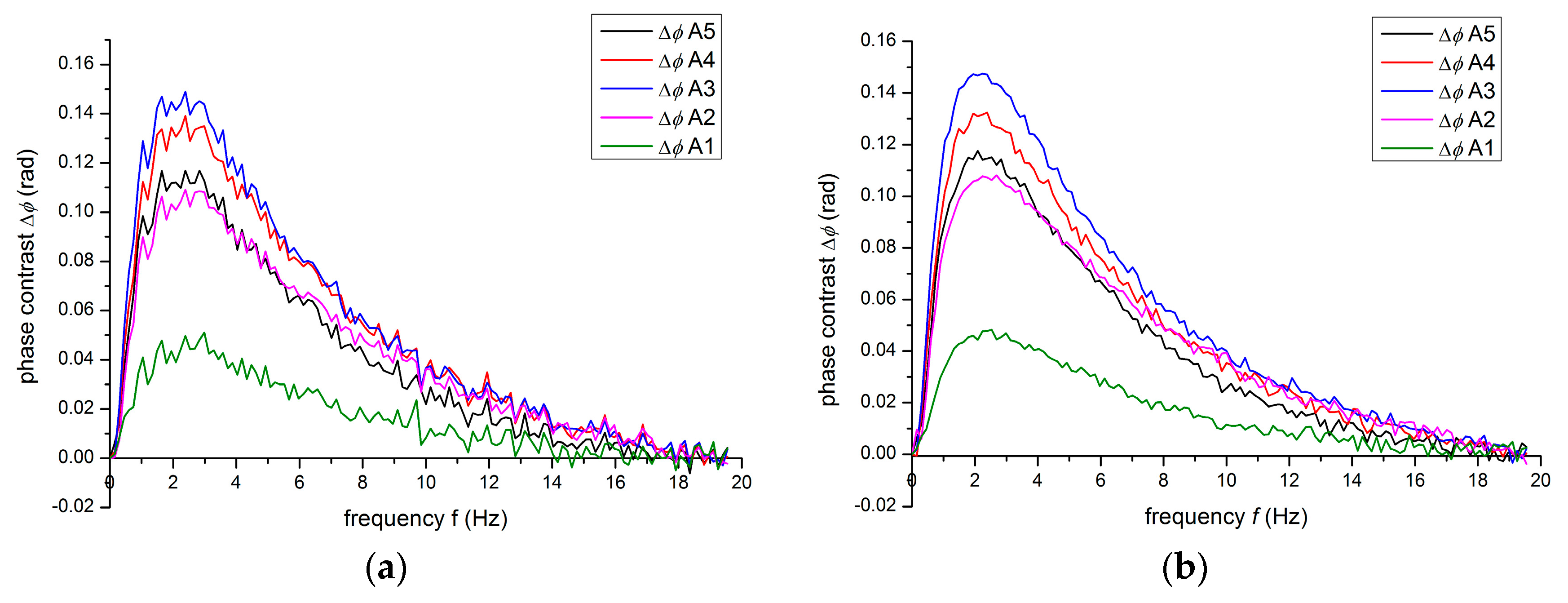
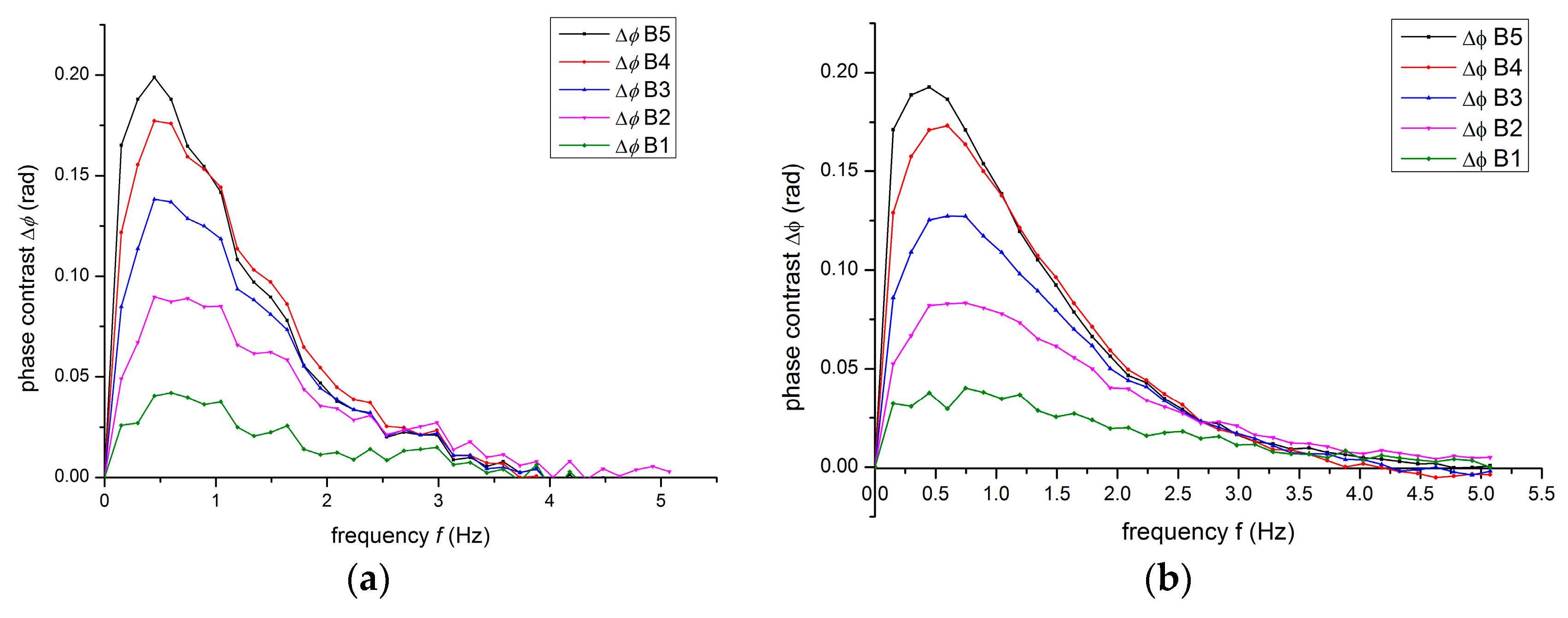
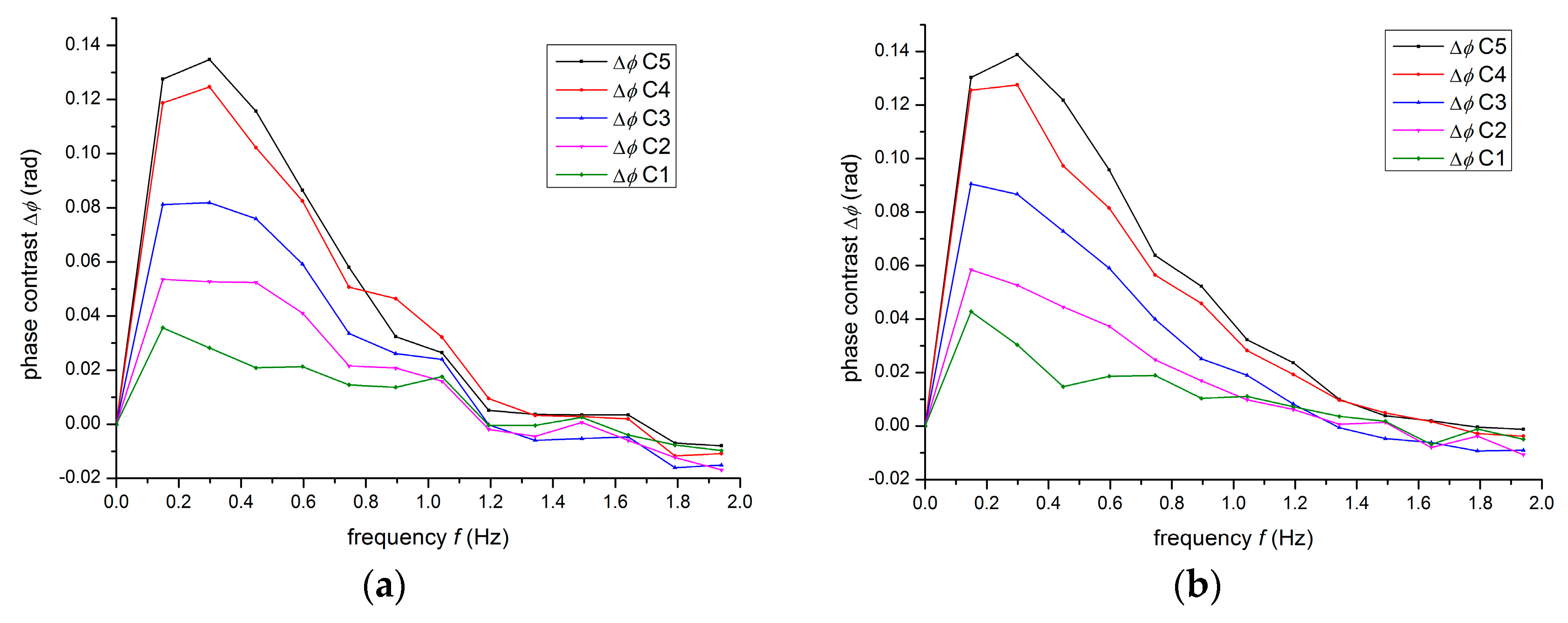
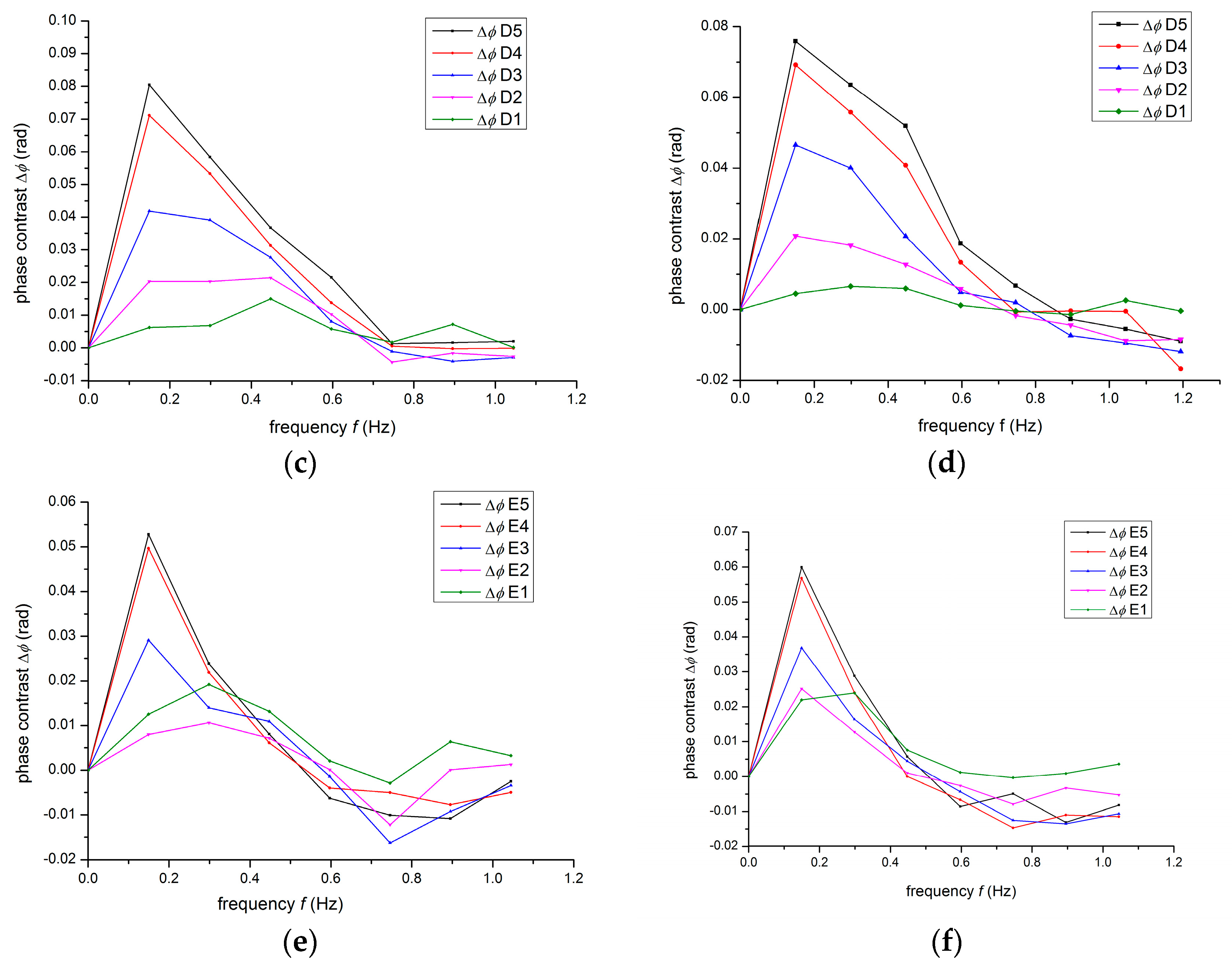
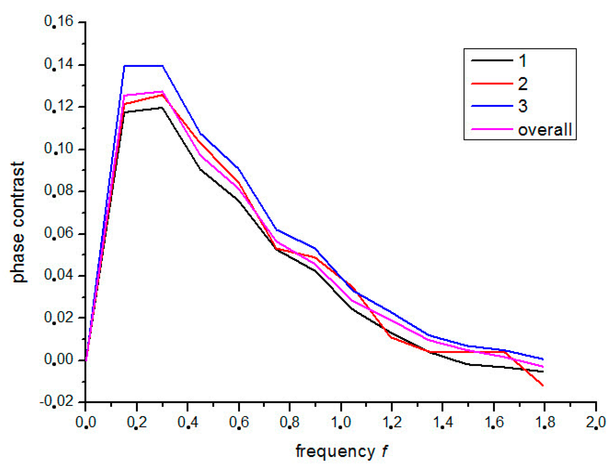
3.2. Depth Retrieval with Blind Frequency

The second depth estimation procedure was performed by means of quantitative pulsed phase thermography, investigating the accuracy produced on depth information retrieval from the analysis of the phase data, the phase contrast calculations and the determination of the blind frequency $f_b$. As presented above, when working with temperature data, the selection of the sound area may have an impact on the thermal contrast calculations and this impact can be additionally enhanced in the case of uneven heating. As a result, in the previous case study different sound areas were selected for the retrieval of depth information, minimising the risk of plotting inappropriate temperature–time evolution curves. However, from the qualitative interpretation of phase images, it was observed that the frequency domain analysis greatly increased the background uniformity (as presented in Figure 3b). Based on the aforesaid, the first depth estimation method in the frequency domain was performed by measuring the correspondent phase contrasts between the defective areas and a region acting as the sound area pre-selected from the background (top left corner of the CFRP surface). Additionally, this procedure was repeated by calculating the average phase intensity from all the pixels on the surface (as the overall surface occupied by the defects was much smaller than the field of view). In such a manner, the use of the overall surface as a sound area was also assessed, aiming primary to evaluate the possibility of overcoming the need for a sound area/point selection in similar inspections. For the purposes of this study, similar to the temporal analysis, the phase contrasts profiles were plotted as a function of frequency for all the detected inserts, aiming to define the characteristic frequency point when the phase contrast diverged zero. Additionally, a comparison of sound area selection impact is performed through the two above mentioned procedures. Similar to the presentation of results in the time domain, before continue with the actual depth characterisation procedure, the phase contrast profiles obtained from the study of the CFRP sample are discussed, investigating the influence of depth and size on the produced contrast and the blind frequency determination.

Figure 9 illustrates the phase contrasts produced from the shallowest insertions (Series A), either selecting a random sound area from the background (left column plot) or by using the entire surface as a sound area (right column plot). Similar to the thermal contrast slope function, phase contrasts were plotted only at the region of interest (frequencies region where the defect was visible), removing the information from the frequency spectrum in which only noise variations were appeared. As can be seen from the 1D phase contrast profiles, similar to the thermal data, in general, larger defects produced a greater phase contrast. A deviation can be seen between the phase contrast intensities measured for defects No. 3 and No. 4 (located at the centre of the panel) and that of defect No. 5 (located at the lower edge of the panel). Nevertheless, for depth calculations the parameter of interest is the blind frequency, which as can be seen from the correspondent plots, it is approximately the same regardless the size of the insertion inspected. The comparison of the two procedures used for the determination of the blind frequency, is revealing that an enhanced similarity was produced regarding the phase contrast evolutions either working with the random sound area or the overall surface, thus its selection has a low impact on the measurement of the blind frequency on Series A defects. However, the interesting point observed by this comparison is the fact that less noise content can be observed in the latter case, which is important when the depth of a shallow defect has to be estimated [36]. Nonetheless, a possible approach for eliminating further the produced noise can be based on repeated measurements, normalising the phase contrast plots.

By studying the effects from the detected defects of Series B and as the depth of the detected features was increased, the phase contrast was affected by the detected feature’s size. More specifically, as can be seen in Figure 10, larger detected insertions in Series B produced greater phase contrasts, regardless the selection of the sound area. However, the size of the insertions had an impact only to the produced contrast as all defects at this depth are visible in approximately the same frequency range. The noise reduction observed in the previous inspection through the selection of the whole surface as a sound area can be also seen from the respective plots of Series B defects, as the Figure 10b is much freer of noise with respect to Figure 10b.

The above presented results for Series B insertions were further confirmed from the plot results of the deeper defects of this panel, illustrated in Figure 11. As can be seen from the correspondent plots the greater is the defect depth the shorter is the frequency range in which the defects are obvious. For instance, the insertions of Series C have a frequency range of visibility from the minimum available frequency (0.149 Hz) to approximately 1 Hz, while for the deepest defects (Series E) the corresponding frequency range is between 0.149 Hz to approximately 0.5 Hz. However, shorter detection frequency ranges perform clearer determinations of the blind frequency, thus less noise content is presented in these cases. The plot results presented in Figure 11 further indicate the impact of feature’s lateral dimensions on the produced contrast, as smaller inserts, regardless of their location, produced weaker phase contrast with respect to the larger ones.

From the phase contrast measurements and the determination of the blind frequency, the depths of all the detected defects into the CFRP panel were quantitatively estimated.

Table A2. Depth estimation using blind frequency.

		Sound Area Top Left Corner			Sound Area All Pixels
Def. No	Nominal Depth in ×10−1 mm	Blind Frequency fb (Hz)	Measured Depth z in ×10−1 mm	Error (%)	Blind Frequency fb (Hz)	Measured Depth z in ×10−1 mm	Error (%)
A5	2	14.476	1.74	−13	15.222	1.70	−15
A4	2	15.371	1.69	−15.5	15.222	1.70	−15
A3	2	16.267	1.65	−17.5	15.222	1.70	−15
A2	2	15.222	1.70	−15	15.222	1.70	−15
A1	2	15.073	1.71	−14.5	14.028	1.77	−11.5
B5	4	3.730	3.44	−14	4.029	3.31	−17.2
B4	4	3.880	3.37	−15.7	4.029	3.31	−17.2
B3	4	3.880	3.37	−15.7	4.178	3.25	−18.7
B2	4	3.581	3.51	−12.2	3.581	3.51	−12.2
B1	4	3.880	3.37	−12.2	3.581	3.51	−12.2
C5	6	1.492	5.44	−7.3	1.492	5.44	−7.3
C4	6	1.641	5.19	−13.5	1.492	5.44	−7.3
C3	6	1.044	6.51	8.5	1.193	6.09	1.5
C2	6	1.193	6.09	1.5	1.492	5.44	−7.3
C1	6	1.044	6.51	8.5	1.492	5.44	−7.3
D5	8	0.746	7.70	−3.7	0.746	7.70	−3.7
D4	8	0.596	8.61	7.6	0.596	8.61	7.6
D3	8	0.596	8.61	7.6	0.746	7.70	−3.7
D2	8	0.596	8.61	7.6	0.596	8.61	7.6
D1	8	0.596	8.61	7.6	0.596	8.61	7.6
E5	10	0.447	9.94	−0.6	0.447	9.94	−0.6
E4	10	0.447	9.94	−0.6	0.447	9.94	−0.6
E3	10	0.447	9.94	−0.6	0.447	9.94	−0.6
E2	10	0.447	9.94	−0.6	0.447	9.94	−0.6
E1	10	0.596	8.61	−16.1	0.596	8.61	−16.1

summarises the experimental values of the blind frequencies and the calculated depths as the product of the diffusion length and the correlation factor C = 1.82. In general, frequency domain analysis and phase data manipulation provided an efficient estimation of the inserts depth, regardless their location and size. Additionally, the similarity of results in terms of error production for inserts having the same depth indicates that the potential non-uniform heat deposition on the inspected surface has a negligible impact on the quantitative information retrieval. Moreover, as regards the quantitative information retrieval and their correlation with the investigated depth, it can be generally seen that defects nearer to the surface produced a larger divergence from the actual depth contrary to the deeper ones where the error production was lower. The above remark was somehow expected as it is attributed to the increase noise levels produced as higher is the frequency range of detection, incommoding the accurate detection of the blind frequency.

The comparison of the two different procedures used for the depth measurements with the phase, referring to the two different sound areas selection, indicates that the selection of the entire surface as a sound area either provided similar results with these produced from the random area selection or it was reducing the error production as in the cases of the Series A and C defects. Thus, the use of the overall surface as a sound area primary eliminates the need for a sound area/point selection and secondly might reduce the potential uncertainty produced from a random selection from the background.

Some deviations were further detected on depth determinations for defects of the same depth. For instance, by calculating the Series E defects depth, by setting the whole surface as a reference, this was measured to be 0.994 mm for E2, E3, E4 and E5 defects and 0.861 mm for defect E1. A more careful study of the measured blind frequencies in this case is indicating that the phase contrast deviation from zero was detected very nearly for all the defects. In particular, it was detected at 0.447 Hz in the former case and at 0.596 Hz in the latter one. Taking into consideration that the truncated frequency interval Δf is 0.149 Hz, this means that the error produced in the second case 16.1% (0.6% in the first case) can be possibly attributed as well to the truncated parameters selected to process the acquired sequences, as the frequency is inversely related to the time interval. As a result, and considering that deeper probing in the frequency domain is less affected by noise, depth estimations for deeper defects seem to be more affected by the truncated parameters due to the lower frequency range in which the defects are visible. Finally, as in the case of temporal analysis, source of extra error could be the deviation from the actual thermal properties of the inspected panels.

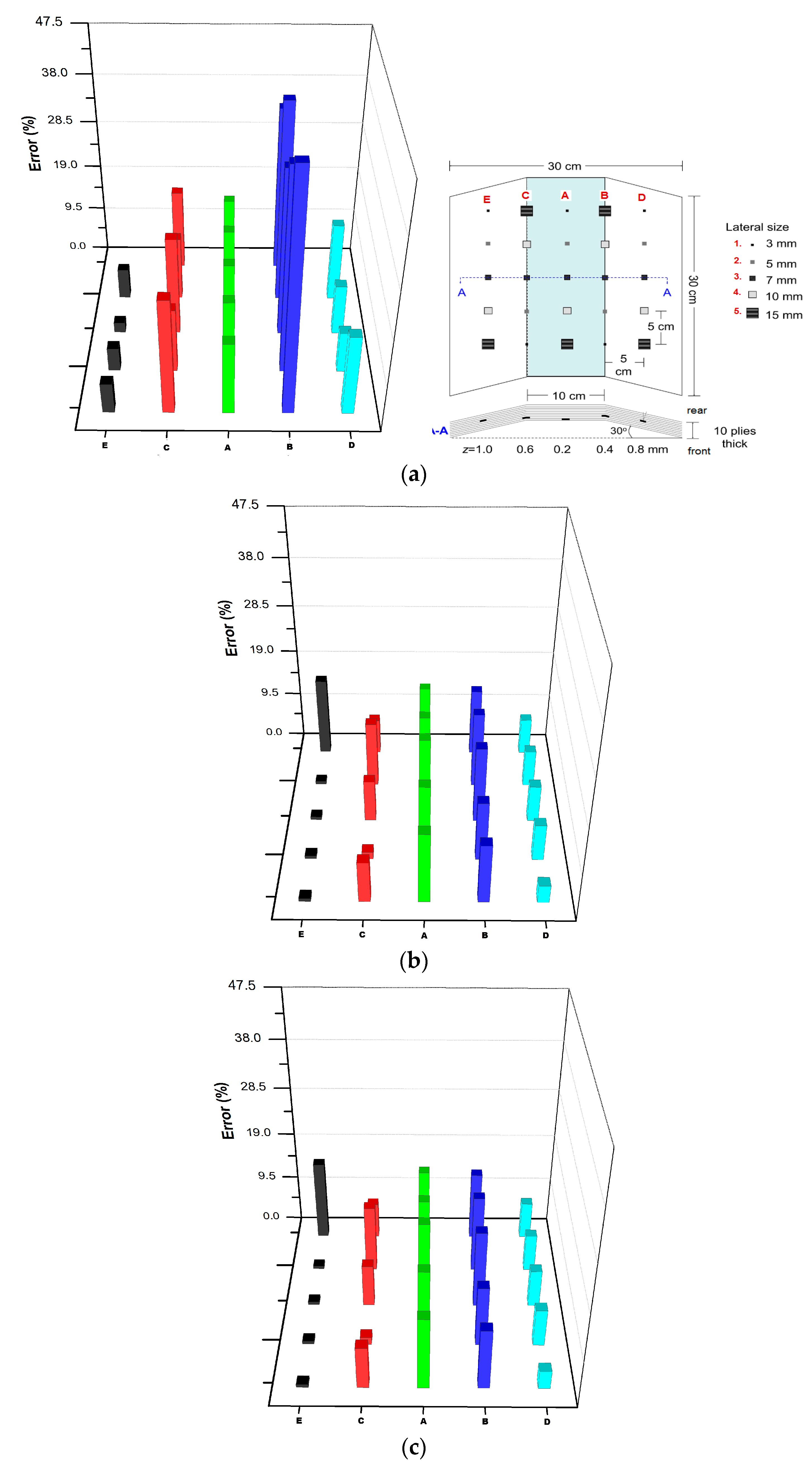
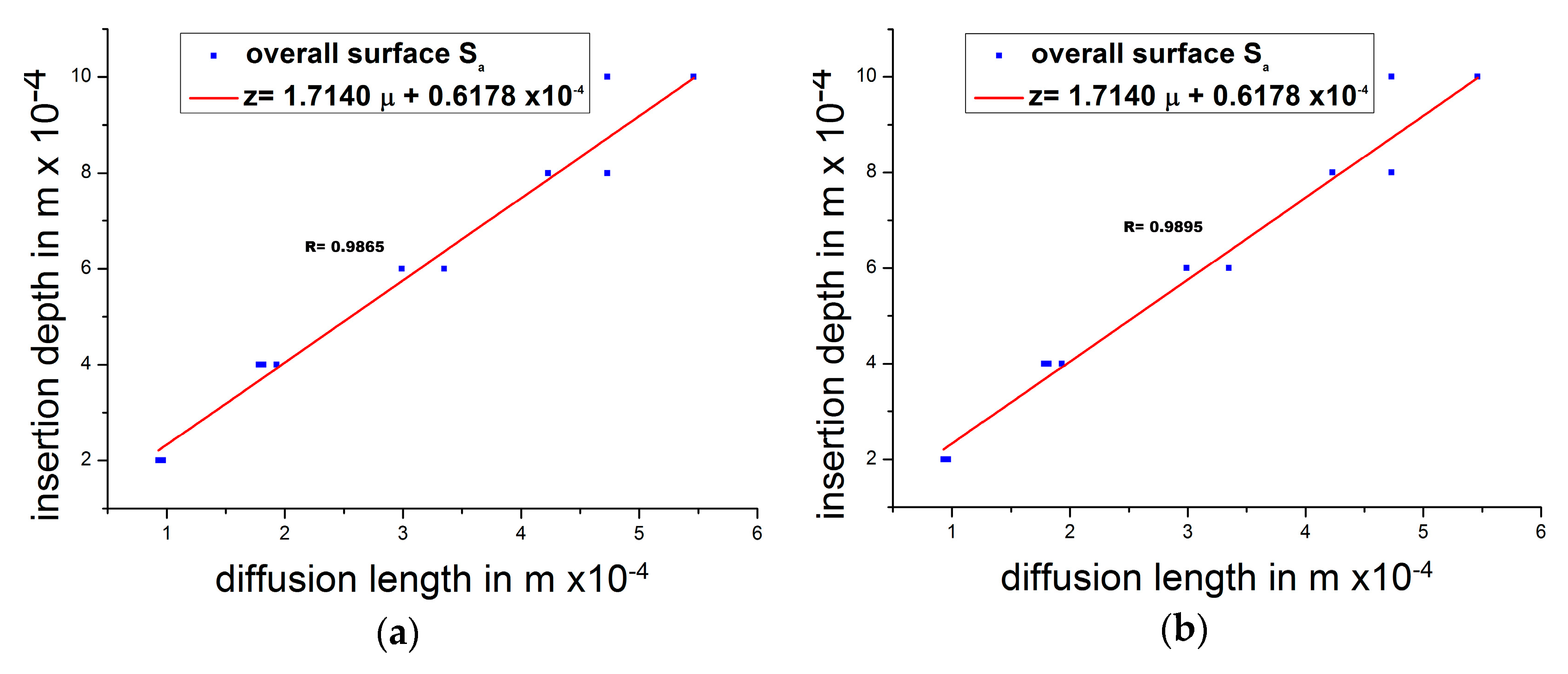
3.3. Comparison of Temporal and Frequency Domain Analysis for the Acquisition of Depth Information

In the previous subsections, results from the quantitative analysis of the CFRP sample were presented, based on the use of the two depth prediction methods. Figure 12 shows a comparison of the measured depths from each individual method in terms of prediction errors. These 3D plots intend to summarise the above discussed quantitative results in a single imaging result, enabling relative comparisons. For this purpose, the scale of the error axis was fixed to be the same in all the three plots, enabling the qualitative evaluation of the produced errors according to the height of each respective bar. The above can be performed as the plots include all the detected defects and the location of each error bar corresponds to the location of the specific insertion with respect to the defect description figure included on the top right side of the figure.

As can be seen from the previously mentioned plots, generally, temporal analysis for depth determination produced larger prediction errors with respect to the correspondent method on the frequency domain. For instance, while peak slope time method provided large divergences on depth prediction of Series B and C defects, this was importantly reduced on the results acquired from the two respective procedures on the frequency domain. Additionally, for some defects mainly in the deeper series which were estimated with a considerable error in the frequency domain, these were not able to be detected and quantified in the temporal domain. Contrarily, the comparison of quantification results acquired by the phase data showed that the selection of the entire surface as sound area either produced similar results with those provided from the random sound area or in some instances this method provided results closer to the actual depth.

As regards the error production and its correlation with the depth, it can be seen that larger errors were produced mainly on Series B and C when working with temperature data, while, in phase data manipulation, a considerable error was produced for defects located at depths of 0.2 mm and 0.4 mm, respectively. Contrarily, more efficient results were produced for Series A, D and E in time domain analysis and for the deeper Series C, D and E in the respective frequency domain analysis. As stated above, the increased errors produced for Series B and C on the temporal analysis can be attributed to the 3D conduction problem, which is not presented on the shallower defects series due to the early time detection and on the deepest ones due to weak signal that they produced. One other hand, the deviations from the actual depth observed from frequency analysis can be attributed to the increased noise levels on the phase contrast plots when the defect is visible in a large frequency range.

4. Evaluation of Analysis Parameters for Depth Prediction

Through the above quantitative analysis of the CFRP component in both the temporal and frequency domains, the acquisition of depth results was achieved and a discussion concerning the possible parameters for error production was done. In the present section, a thorough analysis for the influence degree of these parameters is performed with the aim to assess in a clearer manner how they affect the quantitative depth estimations.

4.1. Selection of Sampling Frequency

From the results presented above it, was observed that a low sampling resolution can be a strong limitation especially in the case of measurements over time for defects close to the surface. For this purpose, new measurements were performed to evaluate the effect of the sampling resolution on the depth results. In particular, a new dataset was collected, monitoring the heat diffusion into the material bulk with a frame rate of 88 Hz. The new sampling frequency contributed to the increase of the temporal resolution reducing the time step from 25 ms to 11 ms. Indicative results from the time domain analysis of the defects in the Series A and B, which produced the largest deviations, are summarised in

Table 2. Depth estimations for the defects of Series A and B.

Def. No	Measured Peak Slope Time in s	Calculated Depth in ×10−1 mm	Error (%)	Def. No	Measured Peak Slope Time in s	Calculated Depth in ×10−1 mm	Error (%)
A5	0.0341	1.97	−1.5	B5	0.2045	4.82	20.5
A4	0.0341	1.97	−1.5	B4	0.1932	4.69	17.2
A3	0.0341	1.97	−1.5	B3	0.1818	4.55	13.7
A2	0.0341	1.97	−1.5	B2	0.2045	4.82	20.5
A1	0.0341	1.97	−1.5	B1	0.2159	4.96	24

. Apart from the change of the sampling resolution, all other experimental parameters were the same as in the previous measurements (i.e., selection of the sound area next to each detected defect).

As can be seen from the results in Table 2, by increasing approximately twice the temporal monitoring resolution, the error production is dramatically reduced. In particular, when studying the heat diffusion with a time step of 25 ms the error production for the defects of Series A was 15%, while by reducing this step to the value of 11 ms the error was calculated to be 1.5%. On the other hand, larger deviations were observed for series’ B defects which however are also reduced if compared with the previous analysis. As discussed in the previous analysis, the large deviations observed on series’ B defects can also be a result of the 3D heat conduction effect, nonetheless from the results in Table 2 it can be seen that a higher sampling frequency can partially overcome the above negative effect.

4.2. Selection of Sound Area

As discussed above, an inappropriate selection of a sound area may affect the calculations for depth accuracy, making this decision a crucial parameter when depth estimations have to be performed. As a result, different procedures were followed for the respective depth measurements in both the time and frequency domain analyses. The plot of Figure 13b presents the thermal contrast slope evolutions to time for defect A1, after selecting three different sound areas as illustrated in Figure 13a. In particular, sound area 1 was selected next to the defect A1, while sound areas 2 and 3 were selected next to the top and vertical edges of the surface, respectively. As can be seen from this indicative plotting result, the different sound areas produced contrast slope evolution curves with different behaviours.

Moreover, the above described procedure was repeated in the frequency domain. An indicative plotting result for the defect C4 is presented in Figure 14. Similar to time domain analysis, the same sound areas 1, 2, and 3 were used as well as the overall surface as a sound area. The comparison of the different plots of Figure 14 is revealing that an enhanced similarity was produced regardless the selection of the sound area, indicating that this parameter has a negligible impact when working with phase data.

4.3. Assessment of Correlation Factor C in Frequency Domain Analysis

As presented in the Introduction, depth quantifications using phase data require knowledge of the correlation factor C, which range from 1.5 to 2, with the value of 1.82 typically adapted in experimental studies. Nevertheless, when investigating anisotropic materials such as the present CFRP panel, the above value may be different, creating uncertainties on the acquired depth results. In this direction, the selection of the correlation factor was assessed in a graphical manner, plotting the nominal depth z of the insertions as a function of the measured diffusion length µ and retrieving the slope of the produced linear function, after linearly fitting these experimental data. Figure 15 presents the correlation results acquired from the two quantification procedures either selecting a sound area from the background (left column plot) or selecting the entire surface as a sound area (right column plot). As stated above, the experimental data were fitted by a least square linear fitting function resulting to high correlation coefficients (0.98). Regardless of the procedure used to estimate the depth, the constant C was measured to be 1.69 in the former case and 1.71 in the latter one (between the range discussed above and very close to the value used in this study). From the graphical assessment of the correlation factor, it can be seen that the value used in this study had a low impact on the acquired results. However, if these graphically retrieved slopes were used for depth quantifications, the results presented on the tables would provide a greater accuracy than this derived using the value of 1.82.

5. Conclusions

In the present study, a CFRP specimen with internal simulated delaminations of various sizes and depth locations was investigated by means of PT for the retrieval of quantitative depth information. Hidden features located in a depth range from 0.2 mm to 1 mm and varying in size from 3 mm to 15 mm were quantitatively characterised using two different analysis procedures through which the impact of different analysis parameters was also assessed. The produced results indicated that the two different analyses provided efficient depth estimations for the inserted features, while the comparison of temporal and frequency domain quantification in terms of error production showed that frequency domain analysis produced measured depths closer to their nominal values. Moreover, the quantification in the frequency domain was further improved by considering the entire surface of the panel as the sound area because the defective zones in the present case occupy a small region with respect to the entire surface. Contrarily, when working with peak slope time and especially when an uneven heating application is presented, depth quantification may be performed selecting different sound areas for depths determinations, ensuring that both the defective and the sound area have received the same amount of heat energy. As regards the selection of the experimental and analysis parameters, time resolution had a great impact on the determination of the characteristic times used for depth estimations and this parameter produced large errors when defects near the surface have to be quantitatively determined. On the other hand, as frequency is inversely proportional to time, the temporal resolution had an impact on the frequency resolution as well. Contrary to temporal data analysis, the low frequency resolution impacted the results of the deeper defects, as the frequency visibility range was lower for these features.

For the continuation of this research, and because these quantification methods require the value of thermal diffusivity α to be available, it is highly recommended to also assess the produced depth accuracy when this value is known. In such a manner, the impact degree of this parameter could be more accurately estimated. Moreover, based on this preliminary study, the application of quantitative infrared thermography for depth prediction in different materials and/or for the characterisation of different defects would provide a clearer view in the assessment of these depth prediction methods. In this direction, a comparative study incorporating different methodologies for depth prediction, such as the Logarithmic Peak Second-Derivative Time method [41], techniques based on the development of numerical modelling [42], or the recently developed Pulse Compression Thermography [43,44,45], which has shown to provide results with enhanced SNR, can define more representatively the strengths and weaknesses of each quantitative technique.

References

1. Maldague, X.P.V. Nondestructive Evaluation of Materials by Infrared Thermography, 1st ed.; Springer-Verlag: London, UK, 1993; pp. 73–99. ISBN 978-1-4471-1995-1. [Google Scholar]
2. Shepard, S.M. Thermal nondestructive evaluation of composite materials and structures. In Comprehensive Composite Materials II, 2nd ed.; Zweben, C.H., Beaumont, P.W.R., Eds.; Elsevier Science: Cambridge, MA, USA, 2017; Volume 7, pp. 250–269. ISBN 978-0-08-100534-7. [Google Scholar]
3. Maierhofer, C.; Röllig, M.; Krankenhagen, R.; Myrach, P. Comparison of quantitative defect characterization using pulse-phase and lock-in thermography. Appl. Opt. 2016, 55, 76–86. [Google Scholar] [CrossRef] [PubMed]
4. Krishnapillai, M.; Jones, R.; Marshall, I.H.; Bannister, M.; Rajic, N. NDTE using pulse thermography: Numerical modeling of composite subsurface defects. Compos. Struct. 2006, 75, 241–249. [Google Scholar] [CrossRef]
5. Theodorakeas, P.; Avdelidis, N.P.; Hatziioannidis, I.; Cheilakou, E.; Marini, R.; Koui, M. Comparative evaluation of aerospace composites using thermography and ultrasonic NDT techniques. In Proceedings of the SPIE 9485, Thermosense: Thermal Infrared Applications XXXVII, Baltimore, MD, USA, 20–24 April 2015. [Google Scholar]
6. Maldague, X.P.V. Theory and Practice of Infrared Technology for Nondestructive Testing, 1st ed.; John-Wiley & Sons: New York, NY, USA, 2001; ISBN 0471181900. [Google Scholar]
7. Peeters, J.; Ibarra-Castanedo, C.; Khodayar, F.; Mokhtari, Y.; Sfarra, S.; Zhang, H.; Maldague, X.; Dirckx, J.J.J.; Steenackers, G. Optimised Dynamic line scan thermographic detection of CFRP inserts using FE updating and POD analysis. NDT E Int. 2018, 93, 141–149. [Google Scholar] [CrossRef]
8. Theodorakeas, P.; Avdelidis, N.P.; Hrissagis, K.; Ibarra-Castanedo, C.; Koui, M.; Malague, X.P.V. Automated transient thermography for the inspection of CFRP structures: Experimental results and developed procedures. In Proceedings of the SPIE 8013, Thermosense: Thermal Infrared Applications XXXIII, Orlando, FL, USA, 25–29 April 2011. [Google Scholar]
9. Avdelidis, N.P.; Ibarra-Castanedo, C.; Theodorakeas, P.; Bendada, A.; Saarimaki, E.; Kauppinen, T.; Koui, M.; Maldague, X.P.V. NDT characterisation of carbon-fibre and glass-fibre composites using non-invasive imaging techniques. In Proceedings of the 10th Quantitative Infrared Thermography Conference (QIRT10), Quebec City, QC, Canada, 27–30 July 2010; pp. 703–710. [Google Scholar]
10. Montanini, R. Quantitative determination of subsurface defects in a reference specimen made of Plexiglas by means of lock-in and pulse phase infrared thermography. Infrared Phys. Technol. 2010, 53, 363–371. [Google Scholar] [CrossRef]
11. Ibarra- Castanedo, C.; Avdelidis, N.P.; Grinzato, E.G.; Bison, P.G.; Marinetti, S.; Chen, L.; Genest, M.; Maldague, X.P.V. Quantitative inspection of non-planar composite specimens by pulsed phase thermography. QIRT 2006, 3, 25–40. [Google Scholar] [CrossRef]
12. James, P.H.; Welch, C.S.; Winfree, W.P. A numerical grid generation scheme for thermal simulation in laminated structures. In Review of Progress in Quantitative Nondestructive Evaluation; Thompson, D.O., Chimenti, D.E., Eds.; Plenum Press: New York, NY, USA, 1989; Volume 8, pp. 801–809. [Google Scholar]
13. Krapez, J.C.; Maldague, X.P.V.; Cielo, P. Thermographic nondestructive evaluation: Data inversion procedures part II: 2-D Analysis and Experimental Results. Res. Nondestruct. Eval. 1991, 3, 101–124. [Google Scholar] [CrossRef]
14. Zeng, Z.; Tao, N.; Feng, L.; Zhang, C. Specified value based defect depth prediction using pulsed thermography. J. Appl. Phys. 2012, 112, 023112. [Google Scholar] [CrossRef]
15. Ibarra-Castanedo, C.; Maldague, X.P.V. Defect depth retrieval from pulsed phase thermographic data on Plexiglas and aluminum samples. In Proceedings of the SPIE 5405, Thermosense XXVI, Orlando, FL, USA, 12–16 April 2004. [Google Scholar]
16. Deemer, C.; Sun, J.G.; Ellingson, W.A.; Short, S. Front-flash thermal imaging characterisation of continuous fiber ceramic composites. In 23rd Annual Conference on Composites, Advanced Ceramics, Materials, and Structures: A: Ceramic Engineering and Science Proceedings; Ustundag, E., Fischman, G., Eds.; The American Ceramic Society: Westerville, OH, USA, 1999; Volume 20, pp. 317–324. [Google Scholar]
17. Theodorakeas, P. Quantitative Analysis and Defect Assessment Using Infrared Thermographic Approaches. Ph.D. Thesis, National Technical University of Athens, Athens, Greece, 2013. [Google Scholar]
18. Ibarra-Castanedo, C.; Gonzalez, D.; Maldague, X. Automatic algorithm for quantitative pulsed phase thermography calculations. In Proceedings of the 16th World Conference on Nondestructive Testing, Montreal, QC, Canada, August 30–September 3 2004. [Google Scholar]
19. Schlichting, J.; Maierhofer, C.; Kreutzbruck, M. Defect sizing by local excitation thermography. QIRT 2011, 8, 51–63. [Google Scholar] [CrossRef]
20. Plotnikov, Y.A.; Winfree, W.P. Advanced image processing for defect visualization in infrared thermography. In Proceedings of the SPIE 3361, Thermosense XX, Orlando, FL, USA, 13–17 April 1998; pp. 331–338. [Google Scholar]
21. Hamzah, A.R.; Delpech, P.; Saintey, M.B.; Almond, D.P. Experimental investigations of defect sizing by transient thermography. Insight 1996, 38, 167–171. [Google Scholar]
22. Bison, P.; Bortolin, A.; Cadelano, G.; Ferrarini, G.; Grinzato, E. Comparison of some thermographic techniques applied to thermal properties characterisation of porous materials. In Proceedings of the 11th Quantitative Infrared Thermography Conference (QIRT2012), Naples, Italy, 11–14 June 2012. [Google Scholar]
23. Maierhofer, C.; Brink, A.; Rolling, M.; Wiggenhauser, H. Quantitative impulse- thermography as non-destructive testing method in civil engineering—Experimental results and numerical simulations. Constr. Build. Mater. 2005, 19, 731–737. [Google Scholar] [CrossRef]
24. Theodorakeas, P.; Avdelidis, N.P.; Cheilakou, E.; Koui, M. Quantitative analysis of plastered mosaics by means of active infrared thermography. Constr. Build. Mater. 2014, 73, 417–425. [Google Scholar] [CrossRef]
25. Zeng, Z.; Li, C.; Tao, N.; Feng, L.; Zhang, C. Depth prediction of non-air interface defect using pulsed thermography. NDT E Int. 2012, 48, 39–45. [Google Scholar] [CrossRef]
26. Almond, D.P.; Patel, P.M. Photothermal Science and Techniques, 1st ed.; Chapman & Hall: London, UK, 1996; ISBN 978-0-412-57880-9. [Google Scholar]
27. Lau, S.K.; Almond, D.P.; Milne, J.M. A quantitative analysis of pulsed video thermography. NDT E Int. 1991, 24, 195–202. [Google Scholar] [CrossRef]
28. Krapez, J.C.; Lepoutre, F.; Balageas, D. Early Detection of thermal contrast in pulsed stimulated thermography. J. Phys. IV 1994, 4, C7.47–C7.50. [Google Scholar] [CrossRef]
29. Krapez, J.C.; Balageas, D.; Deom, A.; Lepoutre, F. Early Detection by stimulated infrared thermography. Comparison with Ultrasonics and Holo/Shearography. In Advances in Signal Processing for Nondestructive Evaluation of Materials; Maldague, X.P.V., Ed.; Springer: Dordrecht, The Netherlands, 1994; Volume 262, pp. 303–321. ISBN 978-94-011-1056-3. [Google Scholar]
30. Plotnikov, Y.A.; Winfree, W.P. Temporal treatment of a thermal response for defect depth estimation. In Review of Progress in Quantitative Nondestructive Evaluation; Thompson, D.O., Chimenti, D.E., Eds.; Plenum Press: New York, NY, USA, 1999; Volume 19, pp. 587–594. [Google Scholar]
31. Favro, L.D.; Han, X.; Kuo, P.K.; Thomas, R.L. Imaging the early time behaviour of reflected thermal wave pulses. In Proceedings of the SPIE 2473, Thermosense XVIII, Orlando, FL, USA, 8–12 April 1996; 1996; pp. 331–338. [Google Scholar]
32. Sun, J.G. Analysis of pulsed thermography methods for defect depth prediction. J. Heat Transf. 2006, 128, 329–338. [Google Scholar] [CrossRef]
33. Ringermacher, H.I.; Archacki, R.J.; Veronesi, W.A. Nondestructive Testing: Transient Depth Thermography. U.S. Patent US5711603, 1998. [Google Scholar]
34. Ibarra-Castanedo, C.; Maldague, X.P.V. Pulsed Phase Thermography Reviewed. QIRT 2004, 1, 47–70. [Google Scholar] [CrossRef]
35. Ibarra-Castanedo, C.; Maldague, X.P.V. Interactive methodology for Optimized Defect characterization by quantitative pulsed phase thermography. Res. Nondestruct. Eval. 2005, 16, 175–193. [Google Scholar] [CrossRef]
36. Ibarra-Castanedo, C. Quantitative subsurface defect evaluation by pulsed phase thermography: Depth retrieval with the phase. Ph.D. Thesis, Université Laval, Quebec City, QC, Canada, 2005. [Google Scholar]
37. Busse, G. Optoacoustic phase angle measurement for probing a metal. Appl. Phys. Lett. 1979, 35, 759–760. [Google Scholar] [CrossRef]
38. Thomas, R.L.; Pouch, J.J.; Wong, H.Y.; Favro, L.D.; Kuo, P.K. Subsurface flaw detection in metals by photoacustic microscopy. Appl. Phys. 1980, 51, 1152–1156. [Google Scholar] [CrossRef]
39. Meloa, C.; Carlomagno, G.M. Recent advances in the use of infrared thermography. J. Meas. Sci. Technol. 2004, 15, R27–R58. [Google Scholar] [CrossRef]
40. Theodorakeas, P.; Avdelidis, N.P.; Ibarra-Castanedo, C.; Koui, M.; Maldague, X. Pulsed thermographic inspection of CFRP structures: Experimental results and image analysis tools. In Proceedings of the SPIE 9062: Smart Sensor Phenomena, Technology, Networks, and Systems Integration, San Diego, CA, USA, 9–13 March 2014. [Google Scholar]
41. Shepard, S.M.; Lhota, J.R.; Rubadeux, A.; Wang, D.; Ahmed, T. Reconstruction and Enhancement of active thermographic image sequences. Opt. Eng. 2003, 42, 1337–1342. [Google Scholar] [CrossRef]
42. Peeters, J.; Ibarra-Castanedo, C.; Sfarra, S.; Maldague, X.; Dirckx, J.J.J.; Steenackers, G. Robust Quantitative Depth Estimation on CFRP samples using active thermography inspection & numerical simulation updating. NDT E Int. 2017, 87, 119–123. [Google Scholar] [CrossRef]
43. Tabatabaei, N.; Mandelis, A. Thermal-wave radar: A novel subsurface imaging modality with extended depth-resolution dynamic range. Rev. Sci. Instrum. 2009, 034902. [Google Scholar] [CrossRef] [PubMed]
44. Ghali, V.S.; Jonnalagadda, N.; Mulaveesala, R. Three-dimensional pulse compression for infrared nondestructive testing. IEEE Sens. J. 2009, 9, 832–833. [Google Scholar] [CrossRef]
45. Silipigni, G.; Burrascano, P.; Hutchins, D.A.; Laureti, S.; Petrucci, R.; Senni, L.; Torre, L.; Ricci, M. Optimization of the pulse compression technique applied to the infrared thermography nondestructive evaluation. NDT E Int. 2017, 87, 100–110. [Google Scholar] [CrossRef]
Figure 1. Schematic representation of defects characteristics and sample description.
Applsci 08 00409 g001
Figure 2. Selection of the sound area for each detected defect in order to calculate the peak slope time from the respective thermal contrast curve in the time domain analysis.
Applsci 08 00409 g002
Figure 3. (a) Raw thermal image of the inspected surface at t = 1.25 s after the application of the heating pulse; and (b) phase image of the inspected surface at f = 0.16 Hz.
Applsci 08 00409 g003
Figure 4. Temporal evolution of: (a) the thermal contrast curves; and (b) the correspondent slope of the thermal contrasts for the detected insertions on the trapezoid surface located to the depth of 0.2 mm (Series A).
Applsci 08 00409 g004
Figure 5. Temporal evolution of: (a) the thermal contrast curves; and (b) the correspondent slope of the thermal contrasts for the detected insertions on the trapezoid surface located to the depth of 0.4 mm (Series B).
Applsci 08 00409 g005
Figure 6. Temporal evolution of: (a) the thermal contrast curves; and (b) the correspondent slope of the thermal contrasts for the detected insertions on the trapezoid surface located to the depth of 0.6 mm (Series C).
Applsci 08 00409 g006
Figure 7. Temporal evolution of: (a) the thermal contrast curves; and (b) the correspondent slope of the thermal contrasts for the detected insertions on the trapezoid surface located to the depth of 0.8 mm (Series D).
Applsci 08 00409 g007
Figure 8. Temporal evolution of: (a) the thermal contrast curves; and (b) the correspondent slope of the thermal contrasts for the detected insertions on the trapezoid surface located to the depth of 1 mm (Series E).
Applsci 08 00409 g008
Figure 9. Phase contrast profiles of the Series A insertions (0.2 mm) after: (a) selecting the left top corner; and (b) the whole surface as a sound area.
Applsci 08 00409 g009
Figure 10. Phase contrast profiles of the Series B insertions (0.4 mm) after: (a) selecting the left top corner; and (b) the whole surface as a sound area.
Applsci 08 00409 g010
Figure 11. Phase contrast profiles for: (a,b) the defects of Series C (0.6 mm); (c,d) the defects of Series D (0.8 mm); and (e,f) the defects of Series E (1 mm). The left side plots correspond to the phase contrasts calculated through the aid of the top left sound area and the right plots correspond to the phase contrasts selecting the entire surface as a sound area.
Applsci 08 00409 g011aApplsci 08 00409 g011b
Figure 12. 3D representation of insertions estimated depth in terms of error production for all the detected defects in the trapezoid specimen through: (a) peak slope time; (b) blind frequency (random sound area); and (c) blind frequency (overall surface).
Applsci 08 00409 g012
Figure 13. (a) Thermal image of the inspected surface showing the regions from which sound areas 1,2, and 3 were selected to calculate the slope of the thermal contrast for Defect A1; and (b) temporal evolution of the correspondent thermal contrast slope curves.
Applsci 08 00409 g013
Figure 14. Phase contrast profiles for defect C4 after selecting three different sound areas from the background and the overall surface.
Applsci 08 00409 g014
Figure 15. Correlation results after: (a) selecting a sound area from the background; and (b) selecting the entire surface as a sound area.
Applsci 08 00409 g015