A Kernel Least Mean Square Algorithm Based on Randomized Feature Networks

Department of Automatic Testing and Control, Harbin Institute of Technology, Harbin 150080, China
*
Author to whom correspondence should be addressed.
Appl. Sci. 2018, 8(3), 458; https://doi.org/10.3390/app8030458
Submission received: 27 January 2018
/
Revised: 11 March 2018
/
Accepted: 15 March 2018
/
Published: 16 March 2018
Abstract
:To construct an online kernel adaptive filter in a non-stationary environment, we propose a randomized feature networks-based kernel least mean square (KLMS-RFN) algorithm. In contrast to the Gaussian kernel, which implicitly maps the input to an infinite dimensional space in theory, the randomized feature mapping transform inputs samples into a relatively low-dimensional feature space, where the transformed samples are approximately equivalent to those in the feature space using a shift-invariant kernel. The mean square convergence process of the proposed algorithm is investigated under the uniform convergence analysis method of a nonlinear adaptive filter. The computational complexity is also evaluated. In Lorenz time series prediction and nonstationary channel equalization scenarios, the simulation results demonstrate the effectiveness of the proposed algorithm.
1. Introduction
In recent years, kernel-based learning has attracted much attention because the designed kernel-based nonlinear algorithm shows extraordinary improvements in performance as compared to the linear one (although at the cost of computational complexity). Representative techniques are the support vector machine (SVM), kernel principal component analysis (KPCA), and the kernel Fisher discriminant (KFD) [1]. Currently, applying the kernel method to the applications of adaptive signal processing is becoming increasingly popular [2,3]. Based on the idea of developing an adaptive filtering technique in the reproducing kernel Hilbert space (RKHS), kernel adaptive filtering (KAF) was proposed; this approach includes a class of nonlinear adaptive filtering algorithms, such as the kernel least mean square (KLMS) algorithm [4], the kernel recursive least squares (KRLS) algorithm [5] and kernel affine projection algorithms (KAPAs) [6]. Compared with other nonlinear adaptive filters, the characteristics of KAF provided by the reproducing kernel Hilbert spaces mainly include the following: (1) general modeling capability; (2) convexity; and (3) flexibility in the tradeoff between performance and complexity. Therefore, kernel-based adaptive algorithms have been widely studied [2,7,8,9,10].
The bottleneck of the kernel adaptive filter is the increase in computational complexity for the training samples during the learning process. It is well established that the kernel function used in the kernel adaptive filter can replace the inner production of the unknown feature mapping function. The implicit mapping mechanism of the kernel trick brings the benefits of the direct use of kernel functions without considering the details of the mapping method from the original space to the high-dimensional feature space. However, the drawback is also quite obvious, as the calculation cost of the kernel matrix will be unacceptable for real-time applications due to the growing weight networks. To restrict the growth of the weight network, several online sparsification criteria were proposed for KAFs to select valid samples in the learning process, such as approximate linear dependency (ALD) [5], the novelty criterion (NC) [11], the surprise criterion (SC) [12], the coherence criterion (CC) [13], the quantization criterion [14], and sparsity-promoting regularization [15,16]. Among these criteria, the quantization criterion-based kernel least mean square (QKLMS) algorithm can perform better in the tradeoff between steady-state error and computational complexity [14]. Although these methods are quite effective in restricting the growth of the weight network, for a nonstationary scenario, the scale of the selected samples will exhibit further growth when the feature of input signals changes because the redundant samples are not pruned during the adaptive learning process. The challenge in limiting the applications of the above improved KLMS algorithm is the lack of online computing ability in a nonstationary environment. To solve the growing problem of the weight network further, the fixed-budget quantized kernel least mean square (QKLMS-FB) algorithm was proposed; the algorithm does not only prune redundant samples but also limits the network size to a preset upper bound [17]. However, the improper setting of the budget may dramatically degrade the accuracy. Further effort is required to determine the appropriate preset budget.
The existing KAFs, which are commonly based on the classic kernel trick, have the drawback of relying on training data due to the implicit mapping mechanism. Based on the scenario of the kernel trick, the transformation does not need to be constructed because the KAFs can be trained and evaluated by computing the kernel function, such as the classical Gaussian kernel, instead of calculating the transformed input vector in reproducing kernel Hilbert space. For implicit mapping-based KAFs, each training sample must be screened by sparsification criteria to limit the growth of the network size. Moreover, in nonstationary situations, all selected samples must be evaluated by the significance criteria to determine whether the new sample should be added to centers and which samples should be pruned. During this process, all selected samples and their significant evaluation results must be saved. A large scale of centers not only brings huge storage costs but also increases the burden of computation.
To overcome the above difficulties, a novel idea of constructing a nonlinear kernel adaptive filter is proposed in this paper. Because the growth of weight network mainly occurs because the accurate mapping relationship of kernel function cannot be obtained, if an approximate kernel mapping function can be obtained, then the iteratively calculated weight coefficients can avoid the growing structure of the weight network. Fortunately, it has been proven that the shift-invariant kernel can be uniformly approximated by the inner products of the randomized features [18,19]. Furthermore, the combination of randomized features with simple linear learning approaches can compete favorably in terms of speed and accuracy with the state-of-the-art kernel-based algorithm [18]. The main advantage of explicitly mapping the input sample into the random Fourier feature space (a relatively low-dimensional space) is that the recursive calculation machine of the linear adaptive algorithm can be utilized in each iteration. In addition, the learning process can eliminate the dependence on the historical training data because the feature information of historical data can be stored in the weight coefficients. In fact, random Fourier feature mapping as an effective explicit mapping method has been widely used in classification and regression applications [20,21,22]. As far as we know, it has never been used in the nonlinear adaptive signal processing field. To introduce this method into the kernel adaptive filter, the KLMS algorithm is taken as an example due to its simplicity and effectiveness. A framework of the explicit mapping-based KLMS algorithm is given, and the randomized feature networks-based kernel least mean square (KLMS-RFN) algorithm is presented by introducing an explicit random projection strategy. To exhibit the proposed KLMS-RFN algorithm, the following efforts have been made: (1) within the steady-state analysis framework based on the energy conservation relation, a convergence analysis of the proposed algorithm including the mean square convergence condition and a steady-state error analysis is given; (2) the detailed computation complexity of the KLMS-RFN algorithm is presented; and (3) extensive simulations are conducted to demonstrate the performance of the proposed algorithm.
The remainder of this article is organized as follows. In Section 2, the background information of the KLMS algorithm and the random feature map is introduced. In addition, the unified framework for constructing the explicit-mapped KLMS algorithm and the KLMS-RFN algorithm is presented. The convergence analysis of the proposed KLMS-RFN algorithm is shown in Section 3. The computation complexity is analyzed in Section 4. Simulation results are illustrated in Section 5. Finally, Section 6 presents the conclusion and discussions of proposed approach.
2. The KLMS Algorithm Based on Random Fourier Features
2.1. The KLMS Algorithm
Before introducing the proposed method, the KLMS is briefly described. The KLMS is the combination of the kernel method and the traditional least mean square algorithm [4]. The kernel method can ensure the existence of a representation that maps the elements of space X to the elements of the high-dimensional feature space H. Then, the least mean square algorithm performs linear filtering of the transformed data . The KLMS algorithm is given as follows. The filter output can be represented as
The weight update equation in the high dimensional space is
where is the prediction error, is the step size, and represents transformation of the sample vector into the feature space . The direct computation of the weight update Equation (2) is impractical for the Gaussian kernel because the kernel mapping function is unavailable. However, the weight vector at iteration n can be non-recursively represented by the following equation:
According to Mercer’s theorem, for any kernel, there exists a mapping such that
Therefore, the filter output of KLMS is given by
Thus, to compute the filter output, an appropriate kernel function must be chosen. The most commonly used kernel is the Gaussian kernel given by
where denotes the kernel parameter. The default kernel function used in this paper is the Gaussian kernel. When the Gaussian kernel is chosen, the KLMS algorithm is actually a growing radial basis function (GRBF) network [14]. New input samples are added to the dictionary and are called centers . The centers will increase with the training data, resulting in great computational and storage burdens.
2.2. The Random Fourier Feature Mapping
The randomized feature mapping method was proposed by Rahimi and Recht [18,19] and has been widely used in classification applications [21,23]. The input samples can be mapped into a randomized Fourier feature space, in which the inner product of any two transformed vectors is equivalent to a shift-invariant kernel (such as Gaussian kernel) operation. Assume that there exists a feature map : such that the inner product between a pair of transformed points approximates their kernel evaluation:
To construct the feature space, where the inner product of the randomized features can uniformly approximate the shift-invariant kernel , the inverse Fourier transform of the well-scaled shift-invariant kernel is assumed to be a proper probability distribution, which can be ensured by Bochner’s theorem [24]. In addition, defining , the following formula can be obtained:
such that is an unbiased estimate of when is randomly sampled from the possibility distribution [18]. To obtain the real-valued random feature that meets the condition , the probability distribution and kernel should be real. Therefore, the is substituted by . Furthermore, according to the conclusion of the authors of [25], the mapping relation can be expressed as . To lower the variance of , the map is normalized. Therefore, the real-valued and normalized approximation can be expressed as
where the real-valued random Fourier feature vector . is independent and identically distributed samples drawn from . The parameter M of random Fourier features represents the dimension of an Euclidean inner product space. In addition to the mapping function , the feature mapping function where is also drawn from and b is drawn uniformly from also satisfies the the condition shown by Equation (9).
2.3. Randomized Feature Networks-Based KLMS Algorithm
In this paper, the random Fourier feature is used to construct an online kernel adaptive filtering algorithm. Based on the conclusions made by the authors of [25], the feature map of is better than the map for Gaussian kernel. Therefore, the randomized feature network is constructed based on the mapping function . Without special explanation, the Gaussian kernel is the default kernel function. Thus, the vector is randomly sampled form the Gaussian probability distribution. For the Gaussian kernel with mean 0 and covariance , can be obtained, where is the kernel bandwidth. Before introducing the randomized feature networks-based KLMS algorithm, the unified kernel-based least mean square scheme based on the explicit feature mapping method is given. Distinct from the implicit mapped KLMS algorithm proposed by the authors of [4], the explicit-mapped KLMS algorithm has similar simplicity to the original LMS algorithm because of its ability to work directly with the weights in the relatively low-dimensional space. For the given training sample, set , and consider the learning problem of a nonlinear function :
where is the input vector and d is the output signal. For the kernel function that can be approximated by
the corresponding nonlinear adaptive algorithm can be constructed using the following steps. First, for the given explicit mapping function , the transformed input vector can be represented by , where denotes that the input vector is transformed into the feature space , which is a relatively low-dimensional space. Second, for the nth iteration, substituting into Equation (1) with the feature vector , the filter output can be computed by
where is the weight vector obtained in the th iteration, and the feature vector can be pre-calculated by an approximate mapping function. The update equation of weight vector in the feature space can be expressed as
where is the step size and is the prediction error computed by
Based on the kernel adaptive filter theory, the above equations, including (12)–(14), constitute the basic framework of the explicit-mapped kernel least mean square algorithm. Given the approximate kernel mapping function , the corresponding kernel-based least mean square algorithm can be constructed. In contrast to the weight updating function applied for the implicit map, the weight vector updating function (13) can be directly achieved by computing the feature mapping function, and the feature information of historical samples can be saved in the weight vector during the iteration process instead of storing the important samples. The real-valued random Fourier feature vector is introduced into the explicit mapped KLMS framework in this paper; the corresponding KLMS-RFN algorithm is shown in Algorithm 1.
| Algorithm 1: The KLMS-RFN Algorithm. |
|
The main characteristics of the proposed KLMS-RFN algorithm can be described as follows: Firstly, the algorithm can save much of the storage cost by eliminating the dependence on the input samples because the KLMS-RFN algorithm does not need to store the important samples. Secondly, compared with the implicit mapping-based KLMS algorithm introduced in [4], the computation complexity of the KLMS-RFN algorithm is lower than that of the computing kernel matrix when the size of the selected samples is large. Thirdly, in addition, the KLMS-RFN algorithm can be used as an online learning algorithm in the nonstationary environment because it can overcome the constraints of a growing weight network and the complex process of updating the sample set to track the feature changes of the input signal. Fourthly, it is a uniform framework of the kernel adaptive algorithm based on explicit mapping mechanism, and different explicit mapping methods can be incorporated into this framework to obtain the corresponding nonlinear adaptive algorithm.
3. The Mean Square Convergence Analysis
The convergence performance is the key aspect of an adaptive filter. The energy relation [26] is a unified tool for analyzing the steady state and transient performance of the nonlinear adaptive filter. The energy conservation relation has been used to analyze the convergence performance of the QKLMS algorithm, which is based on the implicit mapping method [14,27]. In this section, we perform the mean square convergence analysis for the KLMS-RFN by studying the energy flow through each iteration. Firstly, the fundamental energy relation is introduced. Secondly, we present a sufficient condition for mean square convergence. Thirdly, lower and upper bounds on the theoretical value of the steady-state excess mean square error are established.
3.1. The Energy Conversion Relation
Consider a learning system that can estimate the nonlinear mapping relation of
where is the mapping function to estimate, is the transformed feature vector of the input, is the weight vector to estimate an optimal vector , and is uncorrelated interference noise. A different mapping method can represent a class of KLMS algorithms. The weight update of the estimator can be expressed as
Subtracting from both sides of Equation (16) yields
where is the weight error vector in iteration n. Define the priori error and the posteriori error as
The relation between the priori error and the posteriori error is
where . Substituting Equation (19) into Equation (18), we have
To obtain the energy conversion relation, square both sides of Equation (20)
3.2. Mean Square Convergence Condition
To achieve the convergence condition, substitute the error relation
into the energy conversion relation (22) and obtain
By taking the expectations of both sides of (24), the following is obtained:
Assume that the disturbance noise is independent and identically distributed (iid), and has a different distribution to the input sequence ; this assumption is commonly used in convergence analysis [14,26]. Thus, we have
where is the variance of . Equation (25) can be rewritten as
To ensure the convergence of the learning system, the following should be satisfied:
i.e.,
Therefore, with the monotonic decrease of the weight error power , the step size should satisfy the following convergence condition:
3.3. Steady State Mean Square Error Analysis
The steady state mean square error (MSE) is an important indicator of the algorithm’s performance, and it can be represented by
because the noise is dependent from the vector . The steady state analysis of the algorithm can be equivalent to obtaining the excess mean square error (EMSE)
Regarding the steady state, the following assumption can be made:
Thus, Equation (27) is simplified as
After derivation, the following is obtained:
The above equation is similar to the steady state MSE results of the linear LMS obtained in [26], confirming the concept that the KLMS is merely the linear LMS in a high-dimensional feature space [4]. To evaluate tighter expressions of the steady state performance, the following two conditions are considered:
- (1)
- When the step size is sufficiently small, the term can be assumed to be far less than . Therefore, for a small , the following is obtained:
- (2)
- When the step size is large (the value is not infinitesimally small to guarantee filter stability), the following independence assumption is required to find the expression for EMSE. At steady-state, the input signal is statistically independent of . Thus, we obtain
4. Computational Complexity
For N memory elements of input vector and M dimensions of random Fourier features, the computational load per iteration of KLMS-RFN algorithm is calculated Table 1.
As shown in Table 1, the computational complexity of the KLMS-RFN algorithm is mainly related to the dimension of the random Fourier features and the input signal vector. When the dimension of input vector is a constant, the computation complexity of KLMS-RFN will be .
Consider the following calculation of kernel function , where denotes a dictionary with D samples and is a D dimensional error vector. The computation requirement of computing the Gaussian kernel includes multiplications, additions, and D calculations. Therefore, the entire computation complexity can be considered . For the QKLMS-FB algorithm, the computation complexity of updating significance is , when D is the network size of QKLMS-FB [17]. According to whether a new center must be added, the corresponding computation complexity of QKLMS-FB will be two times or three times . Therefore, the computational complexity of QKLMS-FB algorithm is not a fixed value during the training process. The detailed comparison of computation complexity between the proposed algorithm and QKLMS-FB is described in the simulation section.
5. Simulations and Results
To evaluate the performance of the proposed KLMS-RFN algorithm, extensive simulations based on chaotic time series prediction and nonlinear channel equalization are conducted. The commonly used Lorenz chaotic time series are generated as the training data to be predicted. Moreover, the nonlinear channel equalization with a time-varying channel and an abrupt change channel are used to demonstrate the advantages of the proposed algorithm. In this simulation, we focus mainly on the nonstationary situations to show the advantages of the proposed algorithm in online applications.
5.1. Lorenz Time Series Prediction
The problem setting for time series prediction is based on the previous five inputs as the input vector to predict the current points . A chaotic time series is a highly nonstationary time series in the real world [28,29]. The Lorenz model can be described as the three ordinary differential equations:
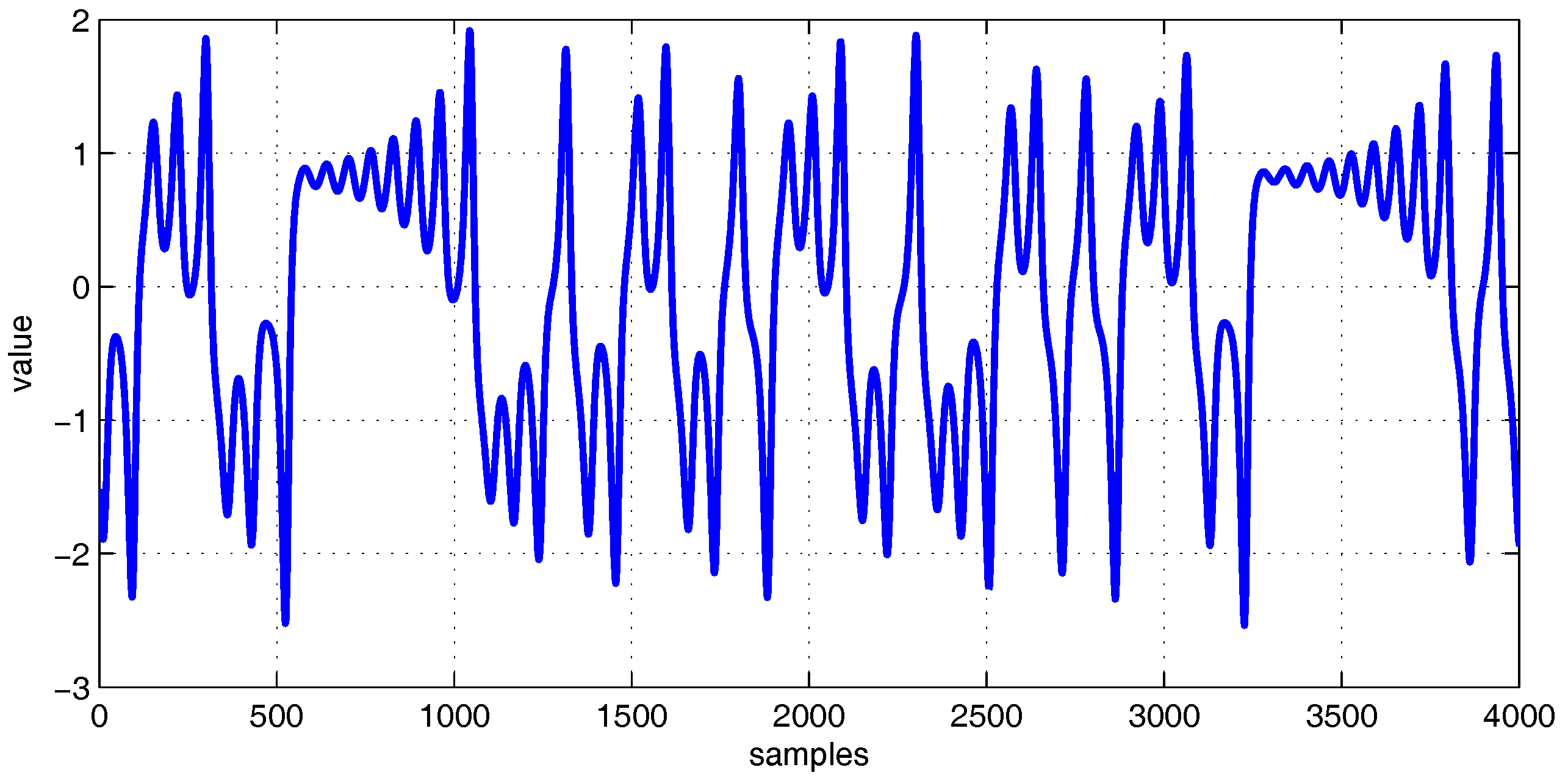
where a, b, and c are set as 10, 8/3, and 28, respectively [30]. The step size in the fourth-order Runge-Kutta method is 0.01. The time delay of the prediction is chosen as 1. The length of generated training samples is 4200, among which the first 200 data are discarded to wash out the initial transient. The left 4000 samples are used as the training set. An extra 200 samples are generated as the testing data to measure the prediction performance. The zero-mean Gaussian white noise with the noise level of 20 dB signal-to-noise ratio (SNR) is added to the time series. For all algorithms compared in this simulation, the step size is set to 0.1. Figure 1 shows the Lorenz time series.
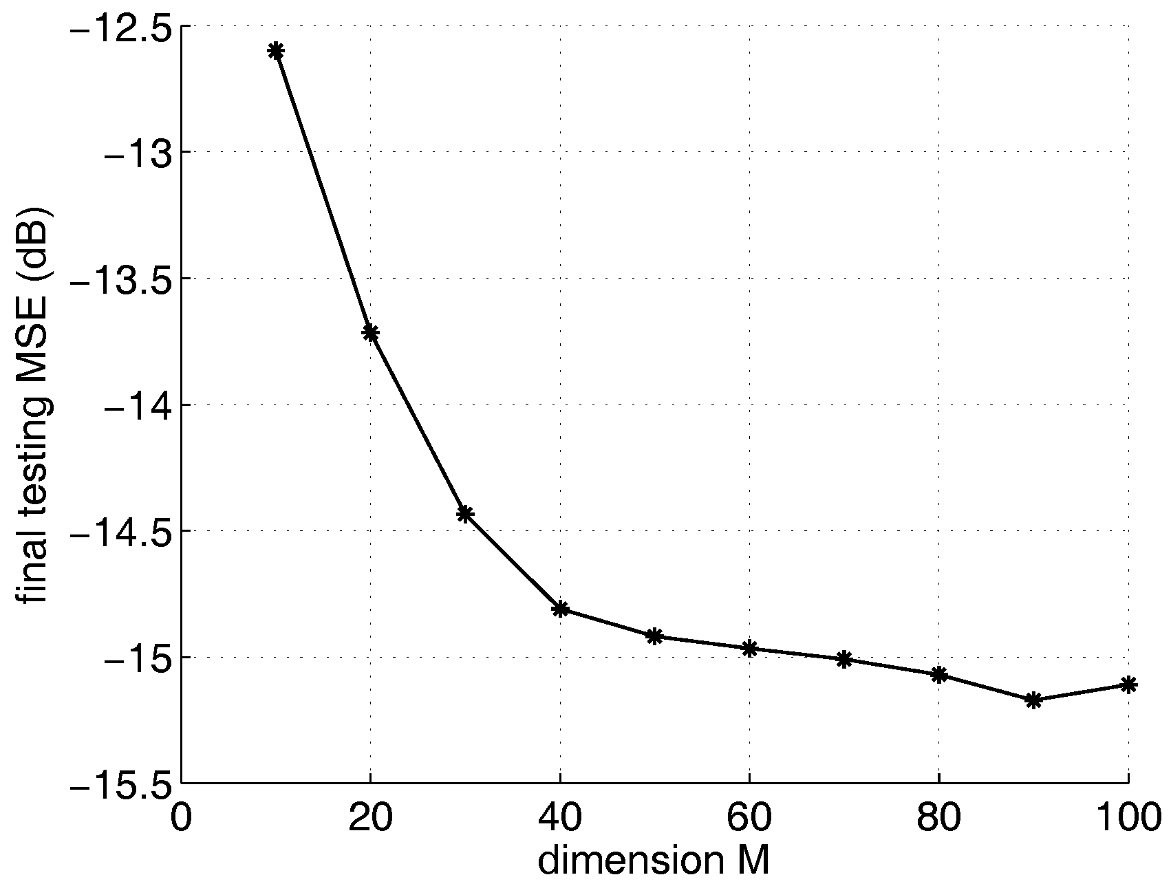
To evaluate the impact of the dimension parameter of KLMS-RFN on the steady state error, the kernel parameter of KLMS-RFN is set to 0.707. After fixing the kernel parameter and the step size, the steady state performance of KLMS-RFN is only affected by the dimension M. The value of parameter M ranges from 10 to 100, with an interval of 10. The smaller MSE equates to better performance in the comparison of different algorithms. As we can see from Figure 2, the final testing MSE of KLMS-RFN becomes better as the dimension increases. However, the performance will not be significantly improved as the dimension increases to a certain extent because the more features that are used to predict the time series, the better the predicting accuracy will be. When the number of dimensions increases to a certain extent, the number of redundant sample features will increase, leading to a slower improvement in accuracy.
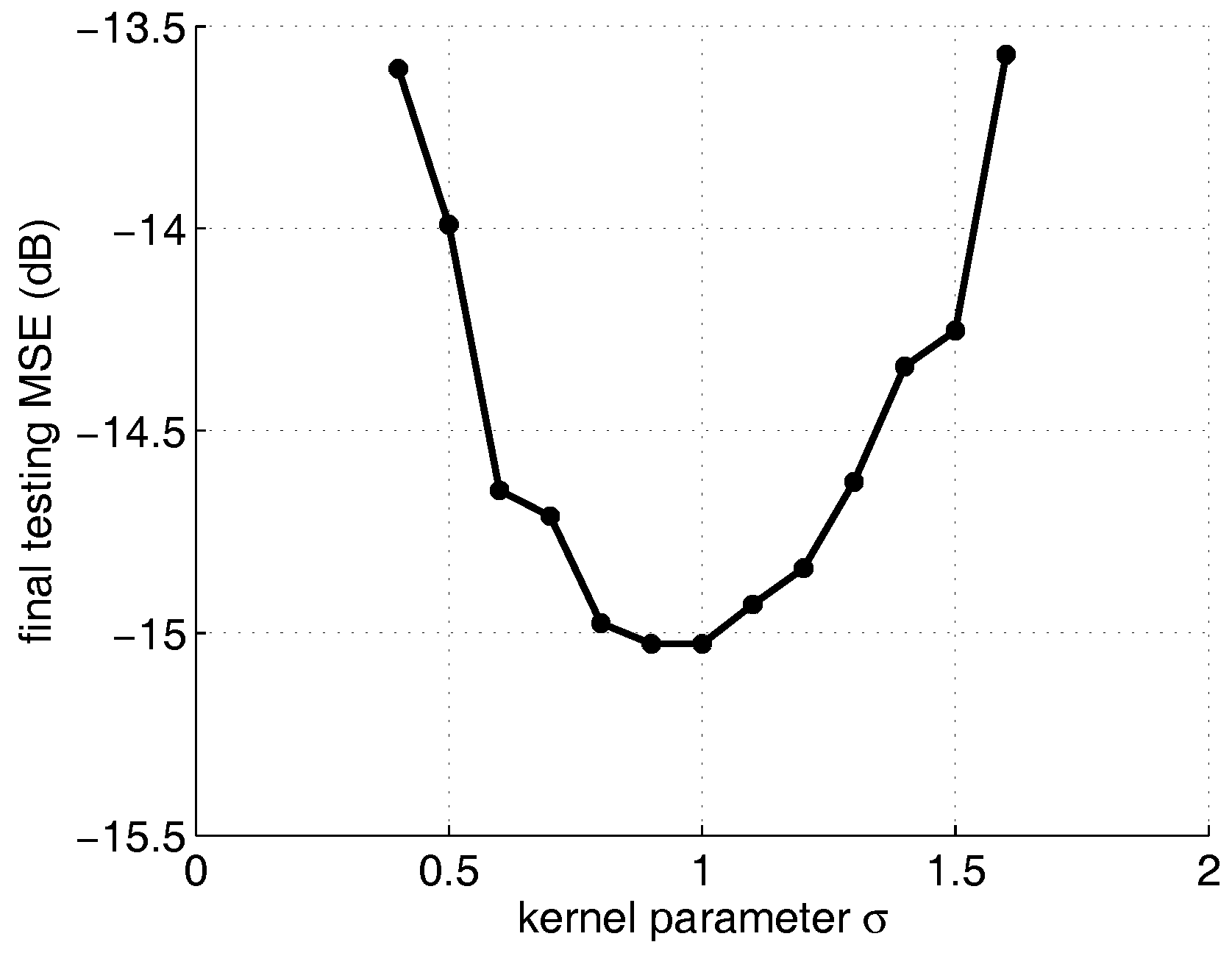
To evaluate the influence of kernel parameter on the steady state error of the KLMS-RFN algorithm, the dimension is chosen as 50, and the value of the kernel parameter ranges from 0.4 to 1.6. Figure 3 shows that the final MSE varies from −11.1 dB to −15.8 dB and finally increases to −14 dB under different . The optimum value of the kernel parameter is 1. Both small and large kernel parameters will lead to accuracy degradation.
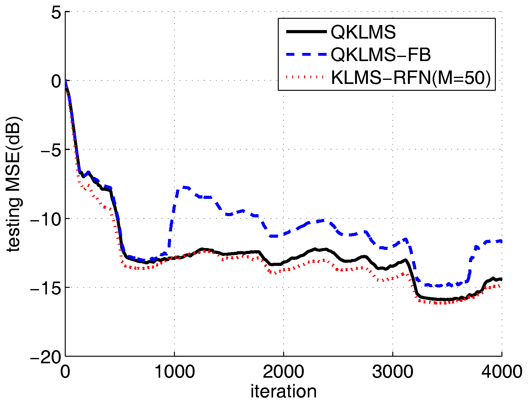
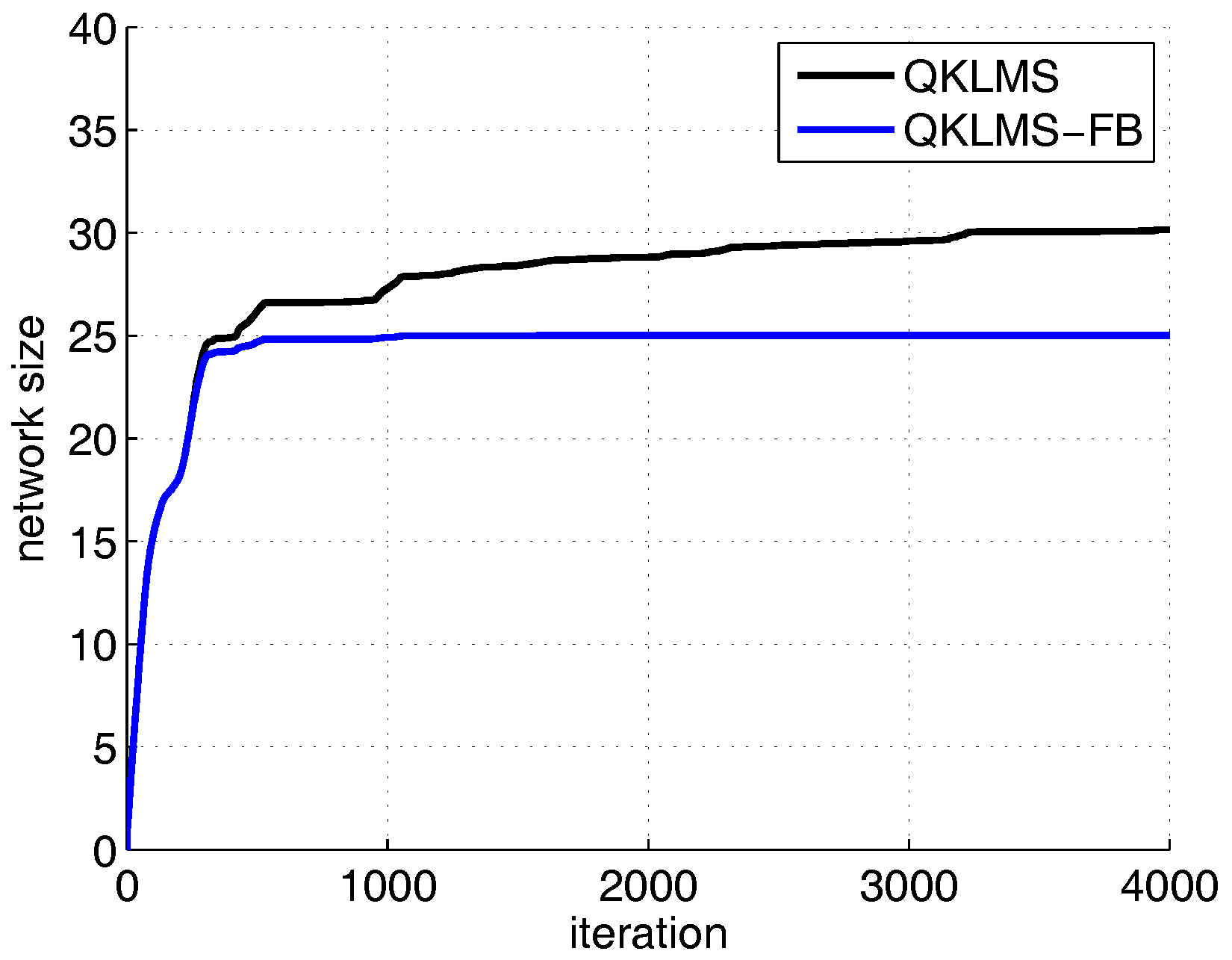
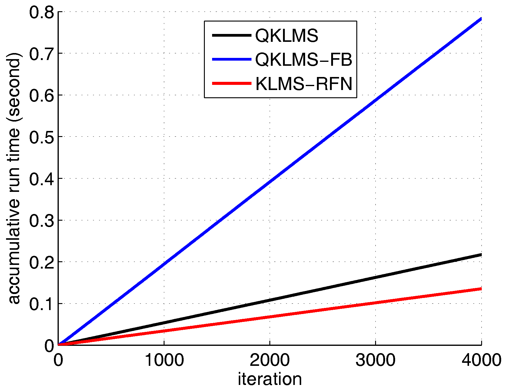
To compare the performance of the proposed algorithm with the QKLMS and QKLMS-FB algorithm, the dimension number of the KLMS-RFN is fixed at 50. The kernel parameter of the QKLMS, QKLMS-FB, and KLMS-RFN is chosen as . The parameters and of the QKLMS-FB are set to 0.4 and 0.96, respectively. The of the QKLMS is set to be the same as for the QKLMS-FB. The budget of the QKLMS-FB algorithm is set to 25. The testing MSE curves and the network size growth curves averaged over 100 Monte Carlo simulations are shown in Figure 4 and Figure 5. The final network size of the QKLMS-FB achieves the preset budget. The final network size of the QKLMS is larger than that of the the QKLMS-FB, which means more memories and computations are required by the QKLMS when calculating the kernel matrix. The final MSE test values for the QKLMS, QKLMS-FB, and KLMS-RFN are −15.37 dB, −12.46 dB, and −15.37 dB, respectively, and are calculated by averaging the last 200 samples. The smaller MSE equates to better steady state performance in the comparison of different algorithms. The proposed algorithm shows the similar performance in accuracy to the QKLMS-FB when the dimension is chosen to be 50. Meanwhile, the accumulative run time is also given. The total run times of the QKLMS, QKLMS-FB, and KLMS-RFN are 0.2171 s, 0.7833 s, and 0.1353 s, respectively, after 4000 iterations. As we can see from Figure 6, the proposed KLMS-RFN is faster than the QKLMS and QKLMS-FB in training.
5.2. Nonlinear Channel Equalization
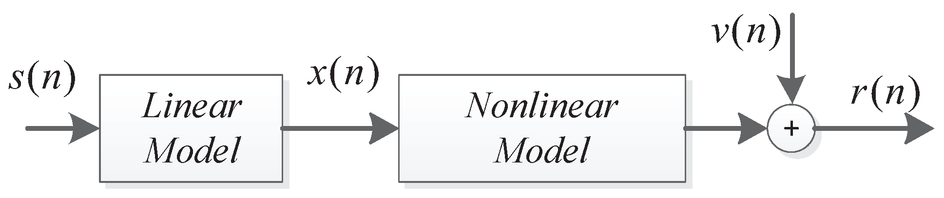
Consider the nonlinear channel consisting of a linear filter and a memory-less nonlinearity, as shown in Figure 7.
5.2.1. Time-Varying Channel Equalization
The time -varying nonlinear channel used in this simulation is often encountered in satellite communication links, as mentioned in [31,32]. The linear channel impulse response is . Here, the channel impulse response is used; such a channel is more likely to be encountered in a real communication system. For the time-varying channel model, the transfer function is defined as
where , and are the time-varying coefficients and are generated by using a second-order Markov model, in which a white Gaussian noise source drives a second-order Butterworth low-pass filter. To generate the time-varying coefficients, the simulation code can be found in [33]. The output of the nonlinear channel is described by
where is 20-dB white Gaussian noise.
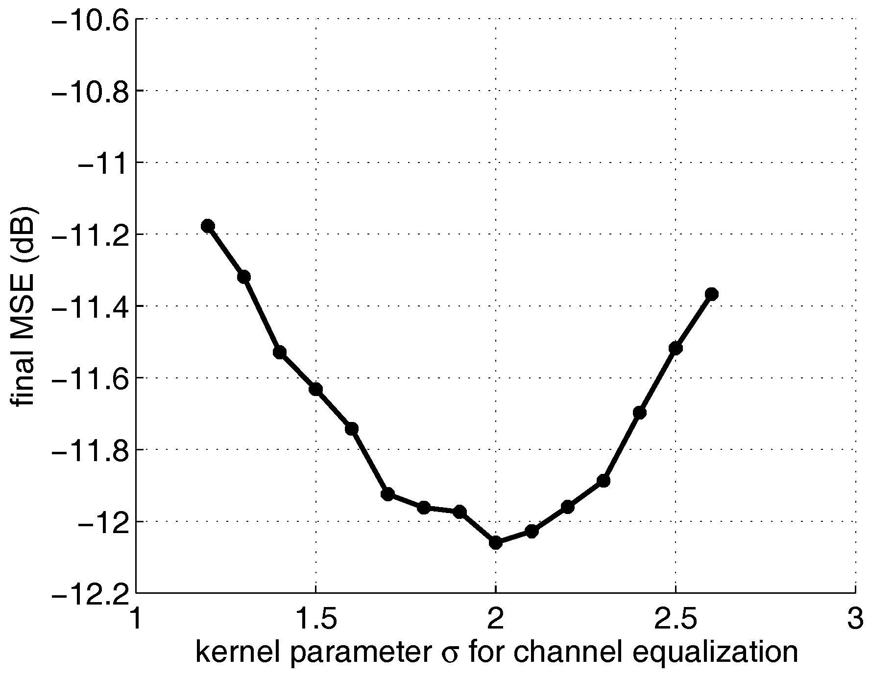
To determine the optimum value of the kernel parameter for a time-varying channel, the dimension of the KLMS-RFN is set to 50. The range of is chosen as 1.2 to 2.6. The MSEs of the KLMS-RFN over 500 Monte Carlo simulations are shown in Figure 8. The optimum value of the kernel parameter for equalizing the time-varying channel used in this simulation is 2. The same rule is used, i.e., that small and large kernel parameters can result in a reduction in accuracy.
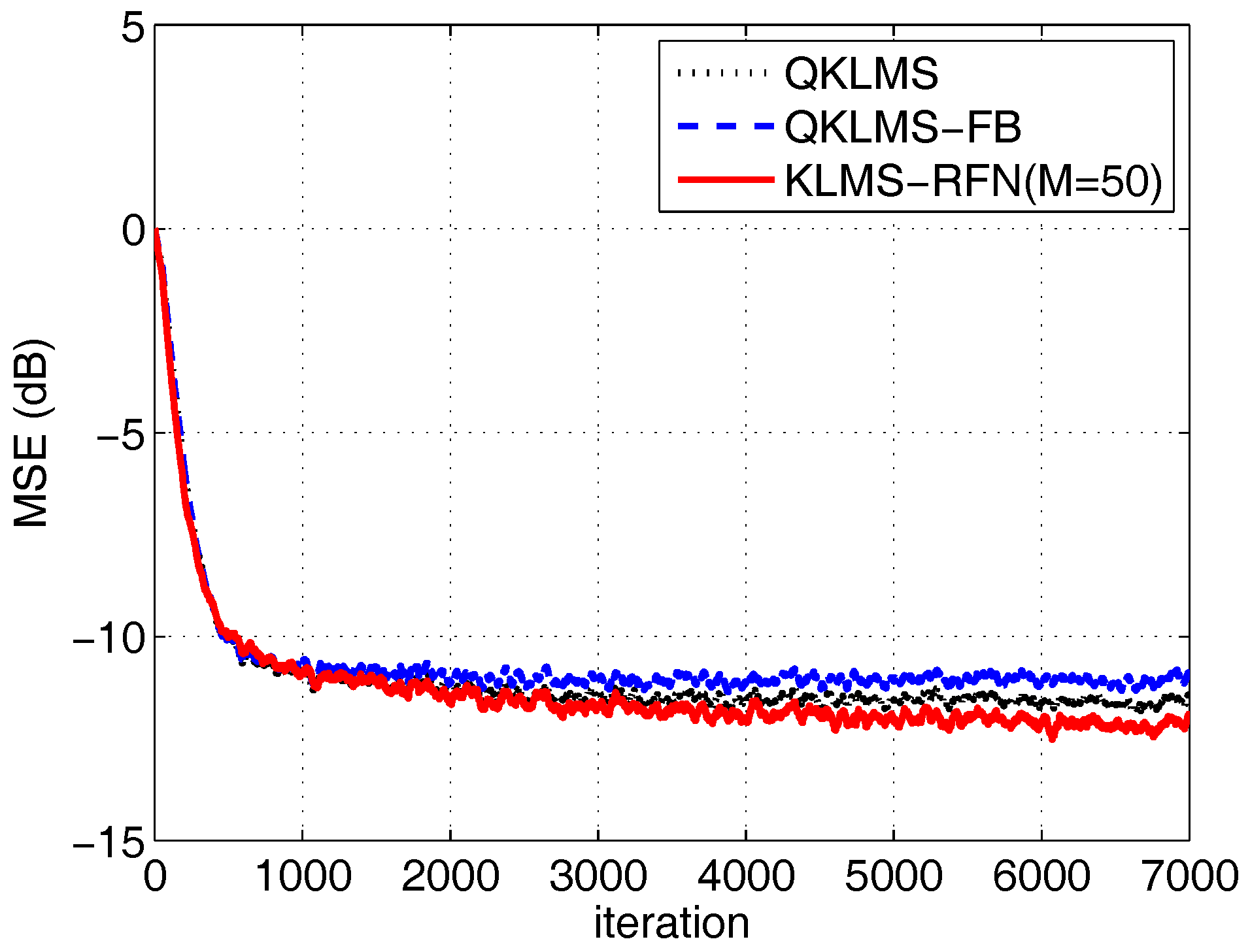
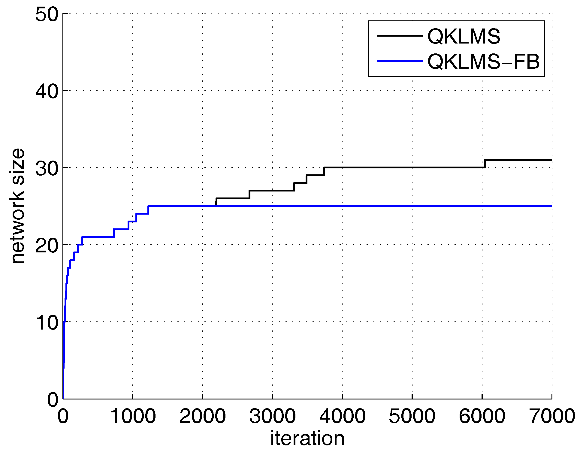
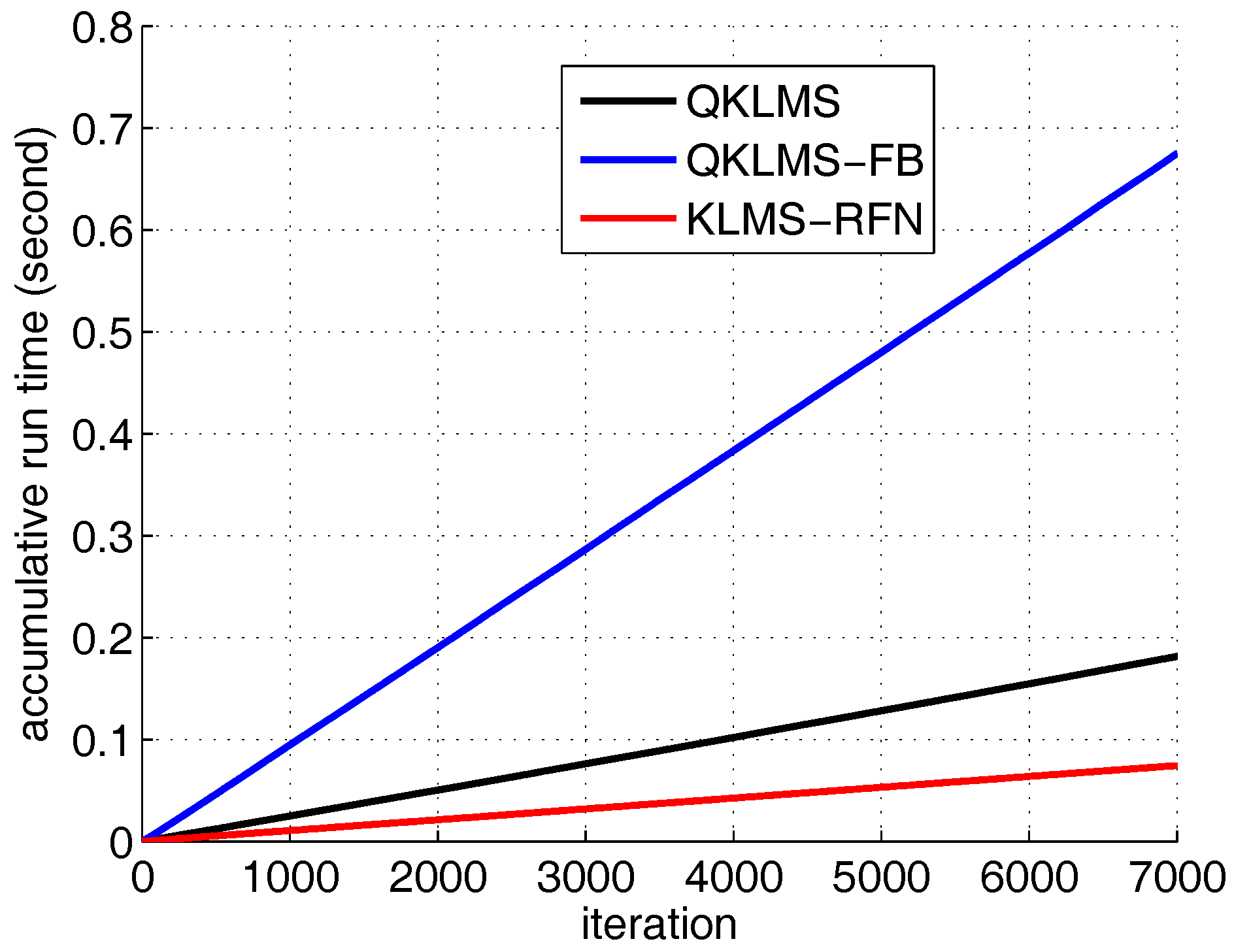
Next, we compare the performance of the KLMS-RFN in equalization with the QKLMS and QKLMS-FB. Their kernel parameters are chosen as 2. All step sizes are set to 0.1. The number of dimensions of the KLMS-RFN is 50. The values of of the QKLMS and QKLMS-FB are both 0.3. The and budget D of the QKLMS-FB are 0.96 and 25, respectively. The MSE curve after 100 independent trials is shown in Figure 9. The network size grown curves of the QKLMS and QKLMS-FB are shown in Figure 10. The network size of the QKLMS-FB achieves its fixed budget, which is lower than the final network size of the QKLMS. The run time curves of the QKLMS, QKLMS-FB, and KLMS-RFN are also given as shown in Figure 11. After 7000 iterations, the total run times of the QKLMS, QKLMS-FB, and KLMS-RFN in time-varying channel equalization are 0.1816 s, 0.6749 s, and 0.0745 s, respectively. The final MSEs of the QKLMS, QKLMS-FB, and KLMS-RFN (M = 50) are −11.55 dB, −10.97 dB, and −12.10 dB, respectively. At the same coverage speed, the KLMS-RFN shows the best performance.
5.2.2. Abruptly Changed Channel Equalization
With several practical nonlinear channel models, the channel impulse response of the linear part can be described by
where the parameter determines the eigenvalue ratio (EVR) of the channel and denotes the difficulty of equalizing a channel [34,35]. Here, is chosen as 2.9 in the first 3000 samples and increases to 3.1 with abrupt change rate for the next 3000 samples and returns to 2.9 for the last 3000 samples. The corresponding normalized channel impulse responses in the z-transform domain are given by
The output of the nonlinear channel is defined by , where represents 20-dB SNR white Gaussian noise. A series of binary signal is used as the desired channel input.
In this simulation, the kernel size of the KLMS-RFN, QKLMS, and QKLMS-FB are set to , and all step sizes are set to . The parameter of the QKLMS and QKLMS-FB are set to be the same with 0.7. The parameter and fixed-budget size of the QKLMS-FB are chosen as 0.96 and 50, respectively. Two learning curves of the KLMS-RFN with dimensions of 50 and 100 are used to demonstrate the performance of the proposed algorithm.
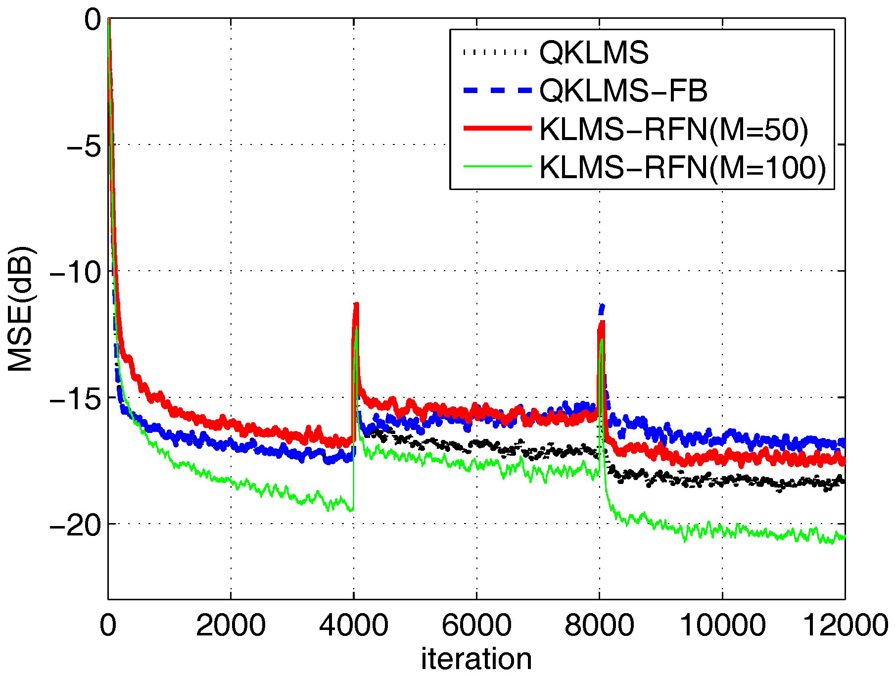
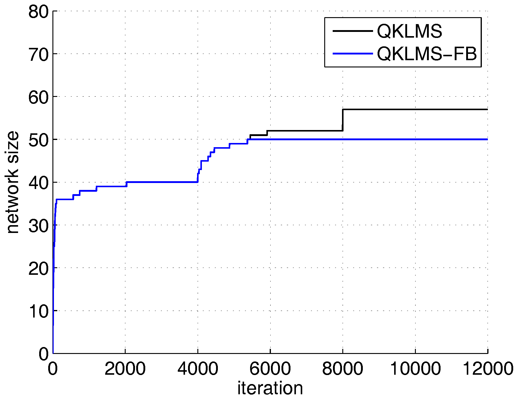
The learning and network size growth curves over 100 Monte Carlo runs are shown in Figure 12 and Figure 13. As indicated in the nonstationary channel equalization with an abrupt change in condition, the following remarks can be made. For the performance of convergence, the proposed method can effectively track the non-stationary change of channel, as shown in Figure 12. On comparing two learning curves of the KLMS-RFN with different dimensions, increasing the number of dimensions did not accelerate the convergence speed of the KLMS-RFN algorithm. This result is reasonable because these features are independent of each other in the process of convergence and because the updating of their weight coefficients is controlled by the step size, which influences the convergence speed.
An analysis of the details is indicated in Figure 12. For the first segment, the QKLMS-FB can achieve the same MSE of −17.13 dB with the QKLMS but with lower computational complexity. After the channel deterioration in segment 2, the QKLMS-FB achieves convergence first and then suffers from performance degradation, with a final MSE of −15.12 at iteration 8000, due to the limitation of the preset budget (see the separation point at almost 4150 in Figure 13). In segment 3 (iteration from 8001 to 12,000), the channel model returns to the initial condition. Compared with the performance in segment 1, the steady-state MSE of the QKLMS-FB algorithm is −17.18 dB, whereas the KLMS-RFN can rapidly achieve MSE values of −16.53 dB (M = 50) and −19.15 dB (M = 100) in the steady state. In segment 3, the QKLMS-FB achieves an MSE value of −16.83 dB, which is worse than the MSE value of −17.18 dB obtained in segment 1. This difference may be due to the limitation in the budget size and the defect in pruning criteria. When the channel model changes, the QKLMS-FB will update the dictionary by pruning some historical centers and adding new centers. During that process, some relatively unimportant new feature samples are retained, and some significant centers cannot be retrieved based on the significance metrics criteria. However, this does not affect KLMS-RFN because the explicit mapping-based algorithm does not rely on historical samples.
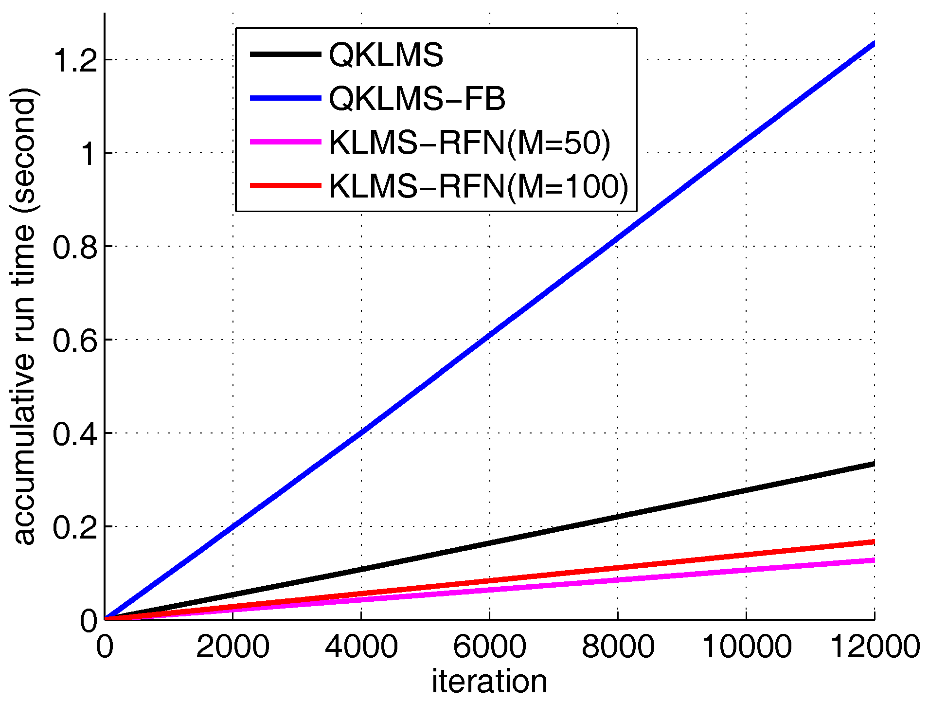
In the steady state performance, the final MSEs of the QKLMS, QKLMS-FB, KLMS-RFN (M = 50), and KLMS-RFN (M = 100) are −18.28 dB, −16.83 dB, −17.52 dB, and −20.55 dB, respectively. The KLMS-RFN (M = 100) achieves the lowest MSE; however, the computational complexity of KLMS-RFN with 100 dimensions is similar to that of the QKLMS-FB. Comparing the aspect of run time, the KLMS-RFN algorithm needs less time in training than the compared algorithm, as shown in Figure 14. After 12,000 iterations, the total run times of the QKLMS, QKLMS-FB and KLMS-RFN in abrupt change channel equalization are 0.3342 s, 1.2349 s, 0.1277 s and 0.1671 s, respectively.
6. Discussion and Conclusions
In this paper, the KLMS-RFN algorithm is proposed to improve the performance of the online kernel-based LMS algorithm in a nonstationary environment by constructing the explicit mapping KLMS framework and introducing the random Fourier features into the kernel adaptive filter. Instead of using the kernel matrix, the KLMS-RFN algorithm can utilize the linear machine for which evaluation process can be realized by simply computing the transformed feature vector in relatively low-dimensional space. Therefore, there is no requirement to establish a dictionary and update it in each iteration, as is the case in the sparsification method-based KLMS algorithm. The mean square convergence and computation complexity analysis are given. The simulation results indicate that the proposed method achieves better performance in nonstationary conditions. The combination of the explicit mapping method and the kernel adaptive filter presents a wide range of possibilities for the further development of the nonlinear adaptive filtering algorithm. Thus, further work may focus on optimizing the random chosen feature vector to achieve better accuracy. In addition, an adaptive strategy may be useful to further improve the convergence performance of the proposed algorithm.
Author Contributions
Yuqi Liu, Chao Sun and Shouda Jiang contributed equally to the development of the research topic and to the writing of the manuscript.
Conflicts of Interest
The authors declare no conflict of interest.
References
- Muller, K.; Mika, S.; Ratsch, G.; Tsuda, K.; Scholkopf, B.; Muller, K.R.; Ratsch, G.; Scholkopf, B. An introduction to kernel-based learning algorithms. IEEE Trans. Neural Netw. 2001, 12, 181. [Google Scholar] [CrossRef] [PubMed]
- Rojo-Alvarez, J.L.; Martinez-Ramon, M.; Munoz-Mari, J.; Camps-Valls, G. Adaptive Kernel Learning for Signal Processing. In Digital Signal Processing with Kernel Methods; Wiley-IEEE Press: Hoboken, NJ, USA, 2018; pp. 387–431. [Google Scholar] [CrossRef]
- Ding, G.; Wu, Q.; Yao, Y.D.; Wang, J. Kernel-Based Learning for Statistical Signal Processing in Cognitive Radio Networks: Theoretical Foundations, Example Applications, and Future Directions. IEEE Signal Process. Mag. 2013, 30, 126–136. [Google Scholar] [CrossRef]
- Liu, W.; Pokharel, P.P.; Principe, J.C. The Kernel Least-Mean-Square Algorithm. IEEE Trans. Signal Process. 2008, 56, 543–554. [Google Scholar] [CrossRef]
- Engel, Y.; Mannor, S.; Meir, R. The kernel recursive least-squares algorithm. IEEE Trans. Signal Process. 2004, 52, 2275–2285. [Google Scholar] [CrossRef]
- Liu, W.; Principe, J.C. Kernel Affine Projection Algorithms. Eurasip. J. Adv. Signal Process. 2008, 2008, 1–12. [Google Scholar] [CrossRef]
- Parreira, W.D.; Bermudez, J.C.M.; Richard, C.; Tourneret, J.Y. Stochastic behavior analysis of the Gaussian Kernel Least Mean Square algorithm. IEEE Trans. Signal Process. 2012, 60, 2208–2222. [Google Scholar] [CrossRef] [Green Version]
- Zhao, J.; Liao, X.; Wang, S.; Chi, K.T. Kernel Least Mean Square with Single Feedback. IEEE Signal Process. Lett. 2015, 22, 953–957. [Google Scholar] [CrossRef]
- Paul, T.K.; Ogunfunmi, T. A Kernel Adaptive Algorithm for Quaternion-Valued Inputs. IEEE Trans. Neural Netw. Learn. Syst. 2015, 26, 2422–2439. [Google Scholar] [CrossRef] [PubMed]
- Haghighat, N.; Kalbkhani, H.; Shayesteh, M.G.; Nouri, M. Variable bit rate video traffic prediction based on kernel least mean square method. IET Image Process. 2015, 9, 777–794. [Google Scholar] [CrossRef]
- Platt, J.C. A Resource-Allocating Network for Function Interpolation. Neural Comput. 1991, 3, 213–225. [Google Scholar] [CrossRef]
- Liu, W.; Park, I.; Principe, J.C. An Information Theoretic Approach of Designing Sparse Kernel Adaptive Filters. IEEE Trans. Neural Netw. 2009, 20, 1950–1961. [Google Scholar] [CrossRef] [PubMed]
- Richard, C.; Bermudez, J.C.M.; Honeine, P. Online Prediction of Time Series Data With Kernels. IEEE Trans. Signal Process. 2009, 57, 1058–1067. [Google Scholar] [CrossRef]
- Chen, B.; Zhao, S.; Zhu, P.; Principe, J.C. Quantized Kernel Least Mean Square Algorithm. IEEE Trans. Neural Netw. Learn. Syst. 2012, 23, 22–32. [Google Scholar] [CrossRef] [PubMed]
- Chen, B.; Zheng, N.; Principe, J.C. Sparse kernel recursive least squares using L1 regularization and a fixed-point sub-iteration. In Proceedings of the 2014 IEEE International Conference on Acoustics, Speech and Signal Processing (ICASSP), Florence, Italy, 4–9 May 2014; pp. 5257–5261. [Google Scholar]
- Gao, W.; Chen, J.; Richard, C.; Huang, J. Online Dictionary Learning for Kernel LMS. IEEE Trans. Signal Process. 2014, 62, 2765–2777. [Google Scholar]
- Zhao, S.; Chen, B.; Zhu, P.; Principe, J.C. Fixed budget quantized kernel least-mean-square algorithm. Signal Process. 2013, 93, 2759–2770. [Google Scholar] [CrossRef]
- Rahimi, A.; Recht, B. Random features for large-scale kernel machines. In Proceedings of the International Conference on Neural Information Processing Systems, Vancouver, BC, Canada, 3–6 December 2007; pp. 1177–1184. [Google Scholar]
- Rahimi, A.; Recht, B. Uniform approximation of functions with random bases. In Proceedings of the Allerton Conference on Communication, Control, and Computing, Urbana-Champaign, IL, USA, 23–26 September 2008; pp. 555–561. [Google Scholar]
- Shakiba, N.; Rueda, L. MicroRNA identification using linear dimensionality reduction with explicit feature mapping. BMC Proc. 2013, 7, S8. [Google Scholar] [CrossRef] [PubMed]
- Hu, Z.; Lin, M.; Zhang, C. Dependent Online Kernel Learning with Constant Number of Random Fourier Features. IEEE Trans. Neural Netw. Learn. Syst. 2015, 26, 2464–2476. [Google Scholar] [CrossRef] [PubMed]
- Boroumand, M.; Fridrich, J. Applications of Explicit Non-Linear Feature Maps in Steganalysis. IEEE Trans. Inf. Forensics Secur. 2018, 13, 823–833. [Google Scholar] [CrossRef]
- Sharma, M.; Jayadeva; Soman, S.; Pant, H. Large-Scale Minimal Complexity Machines Using Explicit Feature Maps. IEEE Trans. Syst. Man Cybern. Syst. 2017, 47, 2653–2662. [Google Scholar] [CrossRef]
- Rudin, W. Fourier Analysis on Groups; Interscience Publishers: Geneva, Switzerland, 1962; p. 82. [Google Scholar]
- Sutherland, D.J.; Schneider, J. On the error of random fourier features. In Proceedings of the Conference on Uncertainty in Artificial Intelligence, Amsterdam, The Netherlands, 12–16 July 2015; pp. 862–871. [Google Scholar]
- Yousef, N.R.; Sayed, A.H. A unified approach to the steady-state and tracking analyses of adaptive filters. IEEE Trans. Signal Process. 2001, 49, 314–324. [Google Scholar] [CrossRef]
- Al-Naffouri, T.Y.; Sayed, A.H. Transient analysis of data-normalized adaptive filters. IEEE Trans. Signal Process. 2003, 51, 639–652. [Google Scholar] [CrossRef]
- Mirmomeni, M.; Lucas, C.; Araabi, B.N.; Moshiri, B.; Bidar, M.R. Recursive spectral analysis of natural time series based on eigenvector matrix perturbation for online applications. IET Signal Process. 2011, 5, 515–526. [Google Scholar] [CrossRef]
- Chandra, R.; Zhang, M. Cooperative coevolution of Elman recurrent neural networks for chaotic time series prediction. Neurocomputing 2012, 86, 116–123. [Google Scholar] [CrossRef]
- Miranian, A.; Abdollahzade, M. Developing a local least-squares support vector machines-based neuro-fuzzy model for nonlinear and chaotic time series prediction. IEEE Trans. Neural Netw. Learn. Syst. 2013, 24, 207–218. [Google Scholar] [CrossRef] [PubMed]
- Kechriotis, G.; Zervas, E.; Manolakos, E.S. Using recurrent neural networks for adaptive communication channel equalization. IEEE Trans. Neural Netw. 1994, 5, 267–278. [Google Scholar] [CrossRef] [PubMed]
- Choi, J.; Lima, A.C.C.; Haykin, S. Kalman filter-trained recurrent neural equalizers for time-varying channels. IEEE Trans. Commun. 2005, 53, 472–480. [Google Scholar] [CrossRef]
- Liang, Q.; Mendel, J.M. Equalization of nonlinear time-varying channels using type-2 fuzzy adaptive filters. IEEE Trans. Fuzzy Syst. 2000, 8, 551–563. [Google Scholar] [CrossRef]
- Patra, J.C.; Meher, P.K.; Chakraborty, G. Nonlinear channel equalization for wireless communication systems using Legendre neural networks. Signal Process. 2009, 89, 2251–2262. [Google Scholar] [CrossRef]
- Xu, L.; Huang, D.; Guo, Y.J. Robust Blind Learning Algorithm for Nonlinear Equalization Using Input Decision Information. IEEE Trans. Neural Netw. Learn. Syst. 2015, 26, 3009–3020. [Google Scholar] [CrossRef] [PubMed]
Figure 1.
The Lorenz time series to be processed.

Figure 2.
The curve of final testing mean square error for the randomized feature networks-based kernel least mean square algorithm (KLMS-RFN) as the dimension M increases from 10 to 100.
Figure 2.
The curve of final testing mean square error for the randomized feature networks-based kernel least mean square algorithm (KLMS-RFN) as the dimension M increases from 10 to 100.

Figure 3.
The final testing MSE curve of KLMS-RFN algorithm with the kernel parameter varying from 0.4 to 1.6.
Figure 3.
The final testing MSE curve of KLMS-RFN algorithm with the kernel parameter varying from 0.4 to 1.6.

Figure 4.
The testing MSE curves of the KLMS-RFN, quantization criterion-based kernel least mean square (QKLMS), and fixed-budget quantized kernel least mean square (QKLMS-FB) algorithms for Lorenz time series prediction.
Figure 4.
The testing MSE curves of the KLMS-RFN, quantization criterion-based kernel least mean square (QKLMS), and fixed-budget quantized kernel least mean square (QKLMS-FB) algorithms for Lorenz time series prediction.

Figure 5.
The network size growth curves of the QKLMS and QKLMS-FB algorithms for Lorenz time series prediction.
Figure 5.
The network size growth curves of the QKLMS and QKLMS-FB algorithms for Lorenz time series prediction.

Figure 6.
The accumulative run times of the QKLMS, QKLMS-FB, and KLMS-RFN algorithms for Lorenz time series prediction.
Figure 6.
The accumulative run times of the QKLMS, QKLMS-FB, and KLMS-RFN algorithms for Lorenz time series prediction.

Figure 7.
The structure of the nonlinear channel.

Figure 8.
The final MSE curve of the KLMS-RFN algorithm with a varied kernel parameter from 1.2 to 2.6 in time-varying channel equalization.
Figure 8.
The final MSE curve of the KLMS-RFN algorithm with a varied kernel parameter from 1.2 to 2.6 in time-varying channel equalization.

Figure 9.
The learning curves of the QKLMS, QKLMS-FB, and KLMS-RFN algorithms in time-varying channel equalization.
Figure 9.
The learning curves of the QKLMS, QKLMS-FB, and KLMS-RFN algorithms in time-varying channel equalization.

Figure 10.
The network size growth curves of the QKLMS and QKLMS-FB algorithms in time-varying channel equalization.
Figure 10.
The network size growth curves of the QKLMS and QKLMS-FB algorithms in time-varying channel equalization.

Figure 11.
The run time curves of the QKLMS, QKLMS-FB, and KLMS-RFN algorithms in time-varying channel equalization.
Figure 11.
The run time curves of the QKLMS, QKLMS-FB, and KLMS-RFN algorithms in time-varying channel equalization.

Figure 12.
The learning curves of the QKLMS, QKLMS-FB, and KLMS-RFN algorithms in channel equalization with an abrupt change in condition.
Figure 12.
The learning curves of the QKLMS, QKLMS-FB, and KLMS-RFN algorithms in channel equalization with an abrupt change in condition.

Figure 13.
The network size growth curves of the QKLMS and QKLMS-FB algorithms in channel equalization with an abrupt change in condition.
Figure 13.
The network size growth curves of the QKLMS and QKLMS-FB algorithms in channel equalization with an abrupt change in condition.

Figure 14.
The run time curves of the QKLMS, QKLMS-FB, and KLMS-RFN algorithms in channel equalization with an abrupt change in condition.
Figure 14.
The run time curves of the QKLMS, QKLMS-FB, and KLMS-RFN algorithms in channel equalization with an abrupt change in condition.


Table 1.
The complexity of the KLMS-RFN algorithm.
| The Number of Calculations of the KLMS-RFN Algorithm. |
|---|
| (1) Calculating random Fourier feature vectors |
| Number of multiplications ; |
| Number of additions ; |
| Number of calculation |
| (2) Calculating the output of the filter |
| Number of multiplications ; |
| Number of additions ; |
| (3) Updating the weight vector |
| Number of multiplications ; |
| Number of additions ; |
| (4) Total calculations |
| Total number of multiplications ; |
| Total number of additions ; |
| Total number of |
© 2018 by the authors. Licensee MDPI, Basel, Switzerland. This article is an open access article distributed under the terms and conditions of the Creative Commons Attribution (CC BY) license (http://creativecommons.org/licenses/by/4.0/).
Share and Cite
MDPI and ACS Style
Liu, Y.; Sun, C.; Jiang, S. A Kernel Least Mean Square Algorithm Based on Randomized Feature Networks. Appl. Sci. 2018, 8, 458. https://doi.org/10.3390/app8030458
AMA Style
Liu Y, Sun C, Jiang S. A Kernel Least Mean Square Algorithm Based on Randomized Feature Networks. Applied Sciences. 2018; 8(3):458. https://doi.org/10.3390/app8030458
Chicago/Turabian StyleLiu, Yuqi, Chao Sun, and Shouda Jiang. 2018. "A Kernel Least Mean Square Algorithm Based on Randomized Feature Networks" Applied Sciences 8, no. 3: 458. https://doi.org/10.3390/app8030458
Note that from the first issue of 2016, this journal uses article numbers instead of page numbers. See further details here.