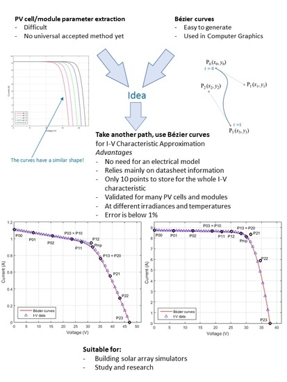
Photovoltaic Cell and Module I-V Characteristic Approximation Using Bézier Curves


Abstract
:
1. Introduction
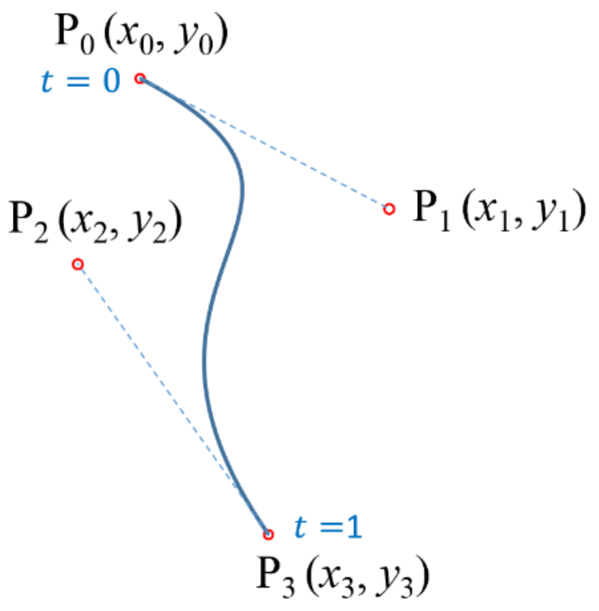
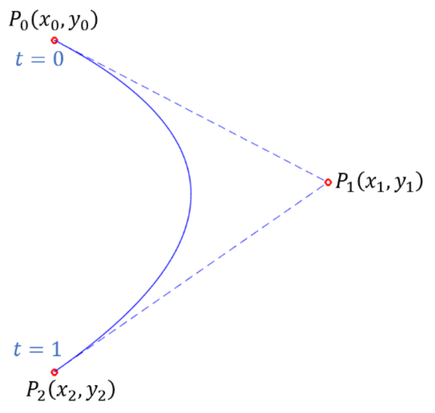
2. Definition of the Bézier Curves
3. Materials and Methods
4. Results
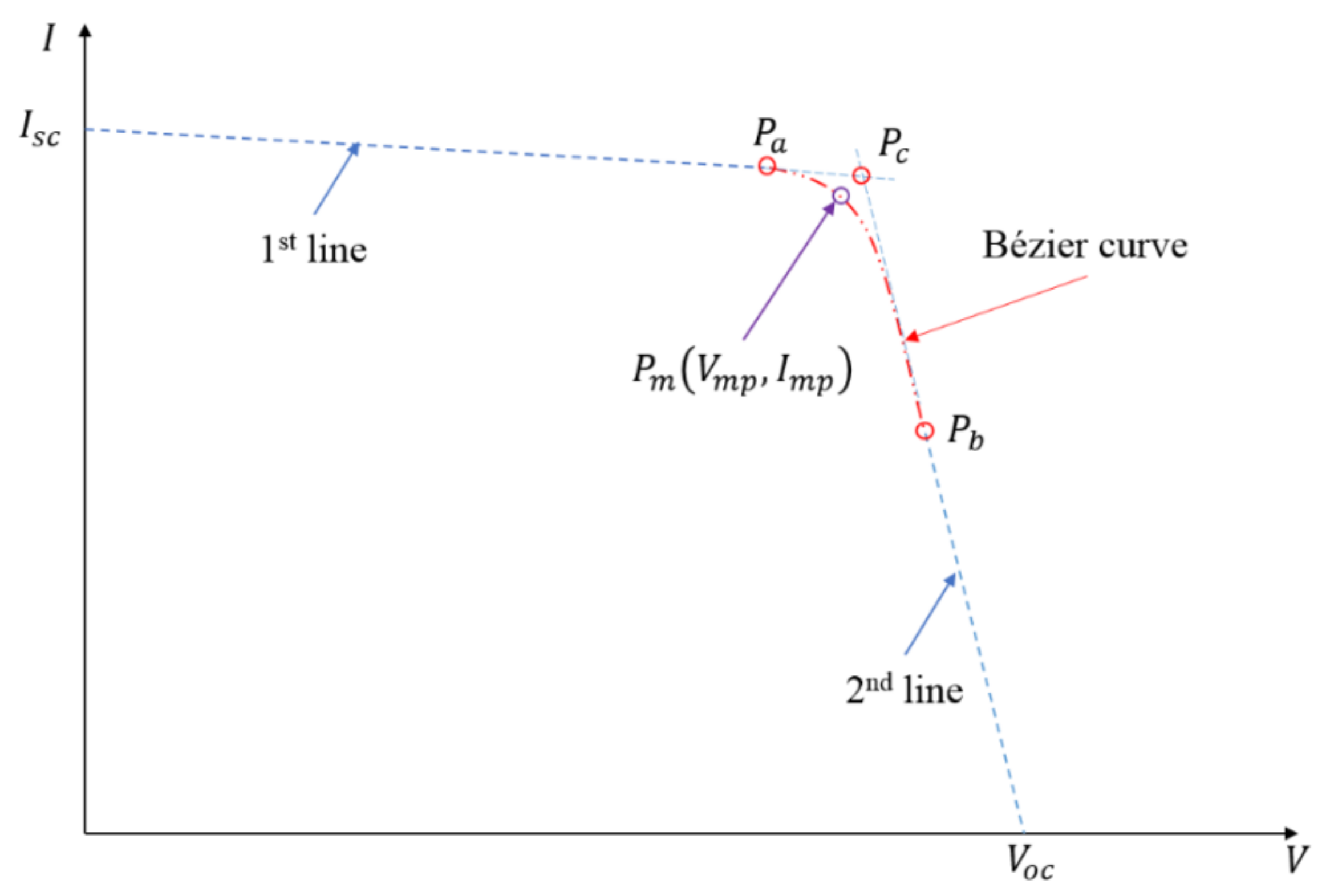
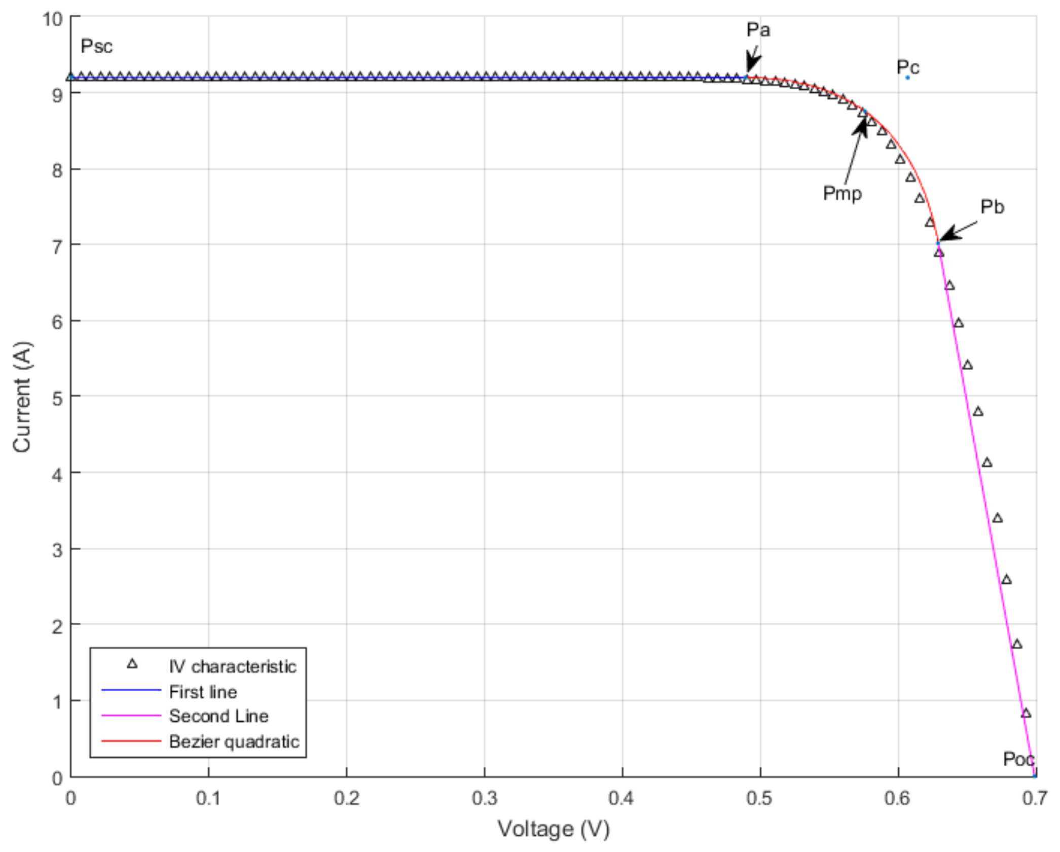
4.1. I-V Characteristic Approximation with Two Segments and a Quadratic Bézier Curve
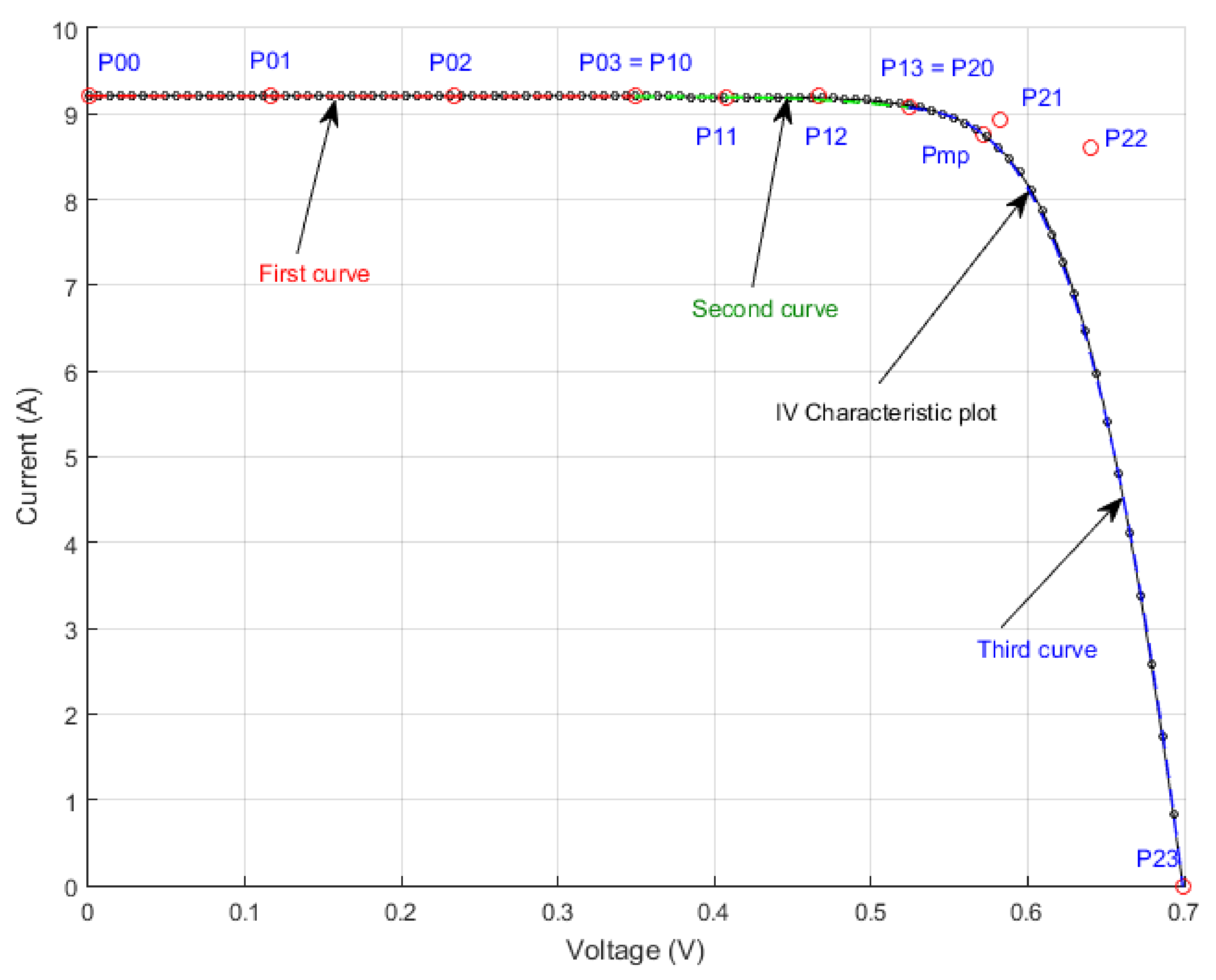
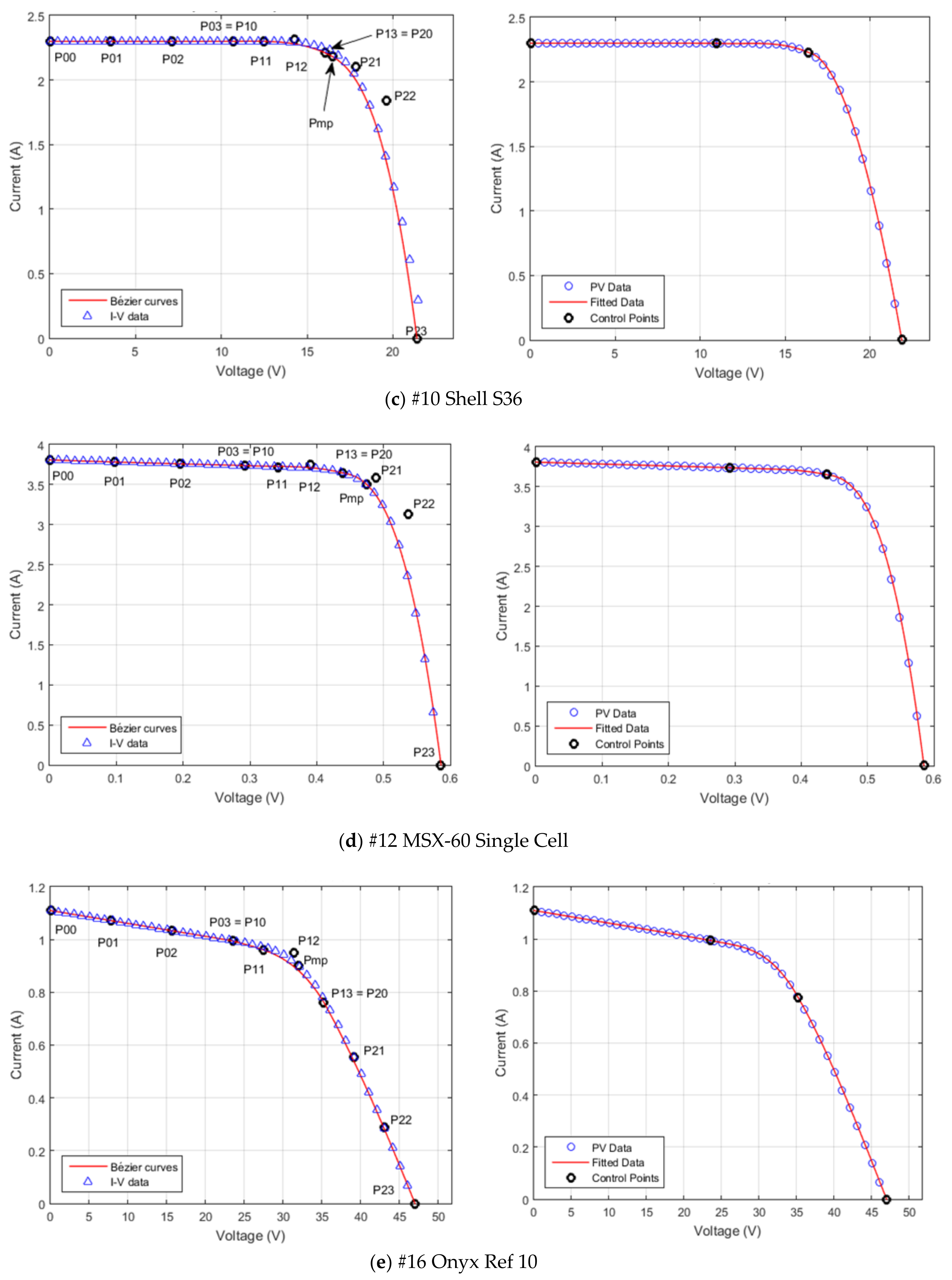
4.2. I-V Characteristic Approximation with Three Cubic Bézier Curves
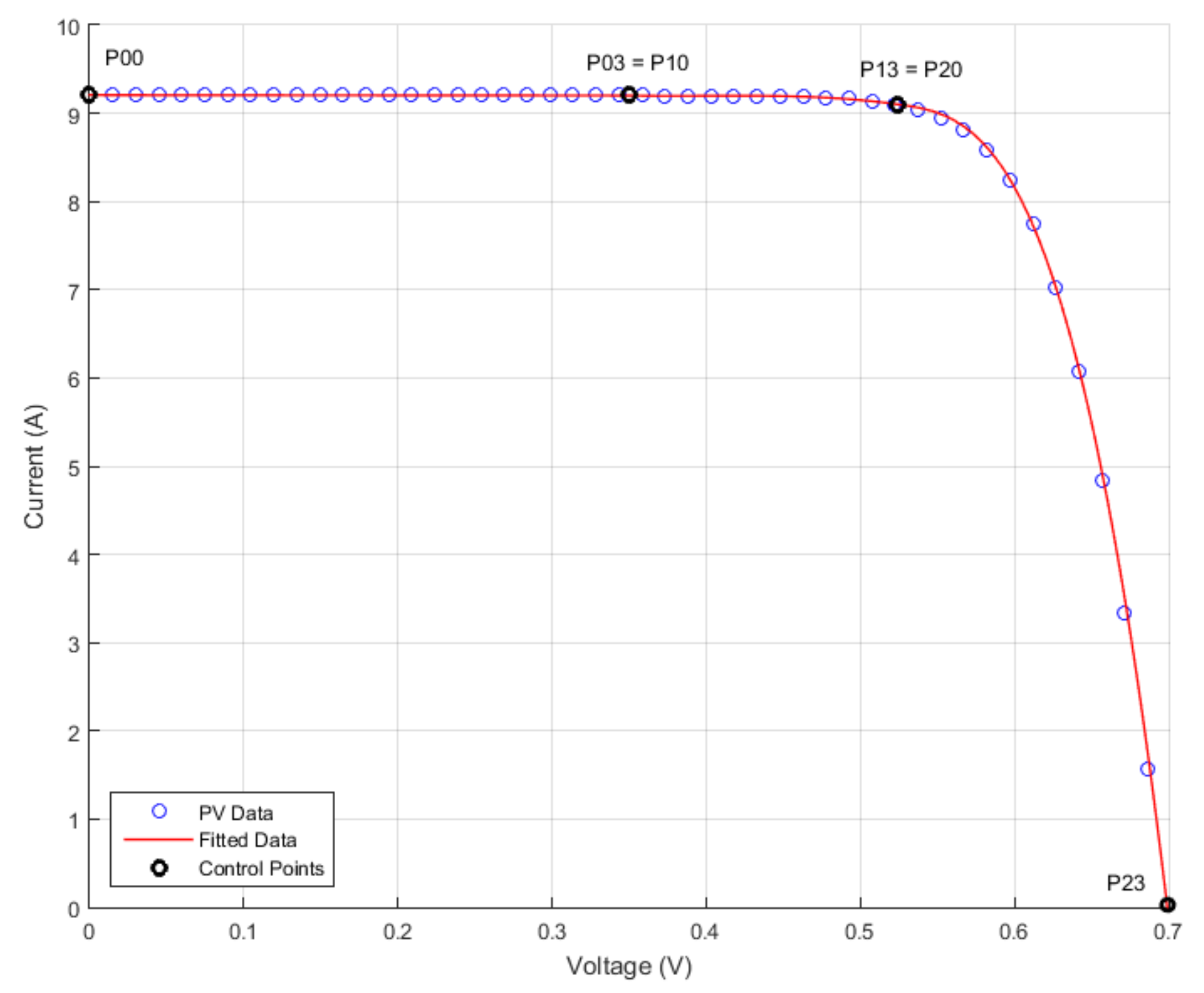
4.3. Data Fitting Using the Least Squares Method
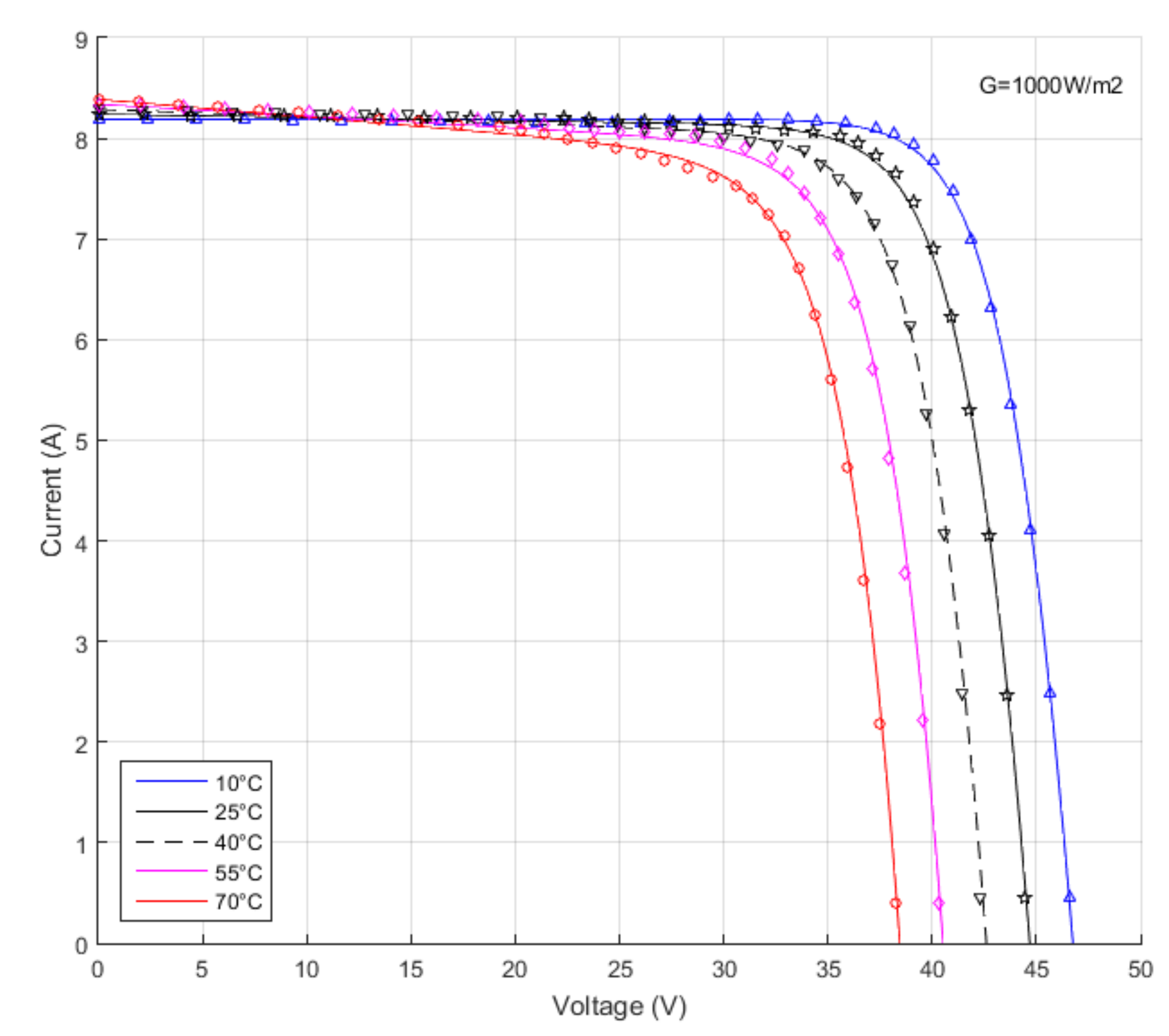
4.4. Parameter Variation
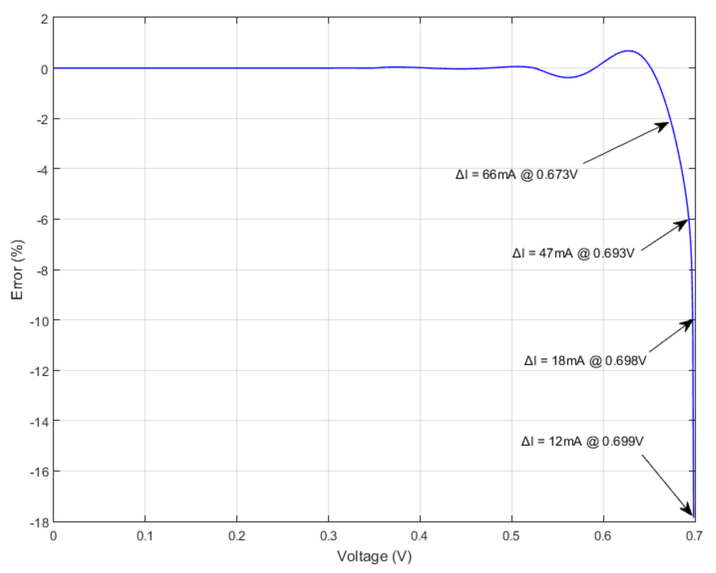
4.5. Final Validation
5. Discussion
6. Conclusions
Supplementary Files
Supplementary File 1Acknowledgments
Author Contributions
Conflicts of Interest
Nomenclature
| Main Symbols | |
| Diode ideality factor | |
| Actual irradiance | |
| Reference irradiance, 1000 W/m2 | |
| Output current | |
| Output current at maximum power point | |
| Short circuit current | |
| Short circuit current 25 °C | |
| Boltzmann constant | |
| Current temperature coefficient, A/K | |
| Voltage temperature coefficient, V/K | |
| temperature exponent | |
| Number of series cells | |
| Maximum output power | |
| Electron charge | |
| Series resistance | |
| Series resistance at 25 °C | |
| Series resistance based on I-V characteristic slope close to | |
| Parallel (shunt) resistance | |
| Parallel (shunt) resistance, at 25 °C | |
| Parallel (shunt) resistance based on I-V characteristic slope close to | |
| Internal temperature, (K) | |
| Reference temperature 298.15 K | |
| Temperature difference | |
| Output voltage | |
| Open circuit voltage | |
| Open circuit reference voltage at 25 °C | |
| Solar cell open circuit voltage | |
| Solar cell open circuit reference voltage at 25 °C | |
| Output voltage at maximum power point | |
| Abbreviations | |
| AM | Air Mass |
| MPPT | Maximum Power Point Tracking |
| PV | Photovoltaic |
| SAS | Solar Array Simulator |
| STC | Standard Test Conditions (cell temp. 25 °C; irradiance 1000 W/m2; air mass 1.5) |
| Greek Symbols | |
| Series resistance temperature coefficient (linear law) |
References
- 4Q 2017 Frontier Power Market Outlook. Available online: https://about.bnef.com/blog/4q-2017-frontier-power-market-outlook/ (accessed on 3 January 2018).
- Solar PV 2018. Available online: https://www.pv-magazine.com/2017/12/01/solar-pv-2018-installs-of-111-gw-a-polysilicon-factory-boom-and-0-30w-for-modules-2/ (accessed on 3 January 2018).
- Phang, J.C.H.; Chan, D.S.H.; Phillips, J.R. Accurate Analytical Method for the Extraction of Solar Cell Model Parameters. Electron. Lett. 1984, 20, 406–408. [Google Scholar] [CrossRef]
- Garrido-Alzar, C.L. Algorithm for extraction of solar cell parameters from I–V curve using double exponential mode. Renew. Energy 1997, 10, 125–128. [Google Scholar] [CrossRef]
- Villalva, M.G.; Gazoli, J.R.; Filho, E.R. Comprehensive Approach to Modeling and Simulation of Photovoltaic Arrays. IEEE Trans. Power Electr. 2009, 24, 1198–1208. [Google Scholar] [CrossRef]
- Babu, B.C.; Gurjar, S. A novel simplified two-diode model of photovoltaic (PV) module. IEEE J. Photovolt. 2014, 4, 1156–1161. [Google Scholar] [CrossRef]
- Cubas, J.; Pindado, S.; de Manuel, C. Explicit Expressions for Solar Panel Equivalent Circuit Parameters Based on Analytical Formulation and the Lambert W-Function. Energies 2014, 7, 4098–4115. [Google Scholar] [CrossRef]
- Chander, S.; Purohit, A.; Sharma, A.; Nehra, S.P.; Dhaka, M.S. A study on photovoltaic parameters of mono-crystalline silicon solar cell with cell temperature. Energy Rep. 2015, 1, 104–109. [Google Scholar] [CrossRef]
- Ishaque, K.; Salam, Z. An improved modeling method to determine the model parameters of photovoltaic (PV) modules using differential evolution (DE). Sol. Energy 2011, 85, 2349–2359. [Google Scholar] [CrossRef]
- Franzitta, V.; Orioli, A.; Di Gangi, A. Assessment of the Usability and Accuracy of the Simplified One-Diode Models for Photovoltaic Modules. Energies 2016, 9, 1019. [Google Scholar] [CrossRef]
- Franzitta, V.; Orioli, A.; Gangi, A.D. Assessment of the Usability and Accuracy of Two-Diode Models for Photovoltaic Modules. Energies 2017, 10, 564. [Google Scholar] [CrossRef]
- Gontean, A.; Lica, S.; Bularka, S.; Szabo, R.; Lascu, D. A Novel High Accuracy PV Cell Model Including Self Heating and Parameter Variation. Energies 2018, 11, 36. [Google Scholar] [CrossRef]
- Cuce, E.; Cuce, P.M.; Karakas, I.H.; Bali, T. An accurate model for photovoltaic (PV) modules to determine electrical characteristics and thermodynamic performance parameters. Energy Convers. Manag. 2017, 146, 205–216. [Google Scholar] [CrossRef]
- Farin, G. A History of Curves and Surfaces in CAGD. In Handbook of Computer Aided Geometric Design; Farin, G.E., Hoschek, J., Kim, M.S., Eds.; Elsevier: Amsterdam, The Netherlands, 2002; pp. 1–22. ISBN 978-0-444-51104-1. [Google Scholar] [CrossRef]
- Farin, G. Curves and Surfaces for CAGD. A Practical Guide, 5th ed.; Academic Press: San Francisco, CA, USA, 2002; pp. 81–95. ISBN 1-55860-737-4. [Google Scholar] [CrossRef]
- Mortenson, M.E. Geometric Modeling, 3rd ed.; Industrial Press: South Norwalk, CT, USA, 2006; ISBN 978-0-831-13298-9. [Google Scholar]
- Farin, G. Shape Representation. In Wiley Encyclopedia of Electrical and Electronics Engineering; 13 July 2007; ISBN 978-0-471-34608-1. Available online: http://onlinelibrary.wiley.com/doi/10.1002/047134608X.W7525.pub2/full (accessed on 30 March 2018). [CrossRef]
- Tromba, D.; Munteanu, L.; Schneider, V.; Holzapfel, F. Approach trajectory generation using Bézier curves. In Proceedings of the 2015 IEEE International Conference on Aerospace Electronics and Remote Sensing Technology (ICARES), Bali, Indonesia, 3–5 December 2015. [Google Scholar] [CrossRef]
- Jalba, A.C.; Wilkinson, M.; Roerdink, J. Shape representation and recognition through morphological curvature scale spaces. IEEE Trans. Image Process. 2006, 15, 331–341. [Google Scholar] [CrossRef] [PubMed]
- Prautzsch, H.; Boehm, W.; Paluszny, M. Bézier and B-Spline Techniques; Spinger: Berlin, Germany, 2002; pp. 9–57. ISBN 3-540-43761-4. [Google Scholar]
- Farin, G. Class A Bézier curves. Comput. Aided Geom. Des. 2006, 23, 573–581. Available online: https://pdfs.semanticscholar.org/1412/bd2310c3f76a31e49129402895564b751e8d.pdf (accessed on 30 March 2018). [CrossRef]
- De Boor, C.; Rice, J.R. Least Squares Cubic Spline Approximation I-Fixed Knots; Dept. of Computer Sciences, Purdue University: West Lafayette, IN, USA, 1968; Available online: ftp://ftp.cs.wisc.edu/Approx/tr20.pdf (accessed on 30 March 2018).
- Levien, R.; Séquin, C. Interpolating Splines: Which is the fairest of them all? Comput. Aided Des. Appl. 2009, 6, 91–102. Available online: http://levien.com/phd/LevienSequinCAD09_014.pdf (accessed on 30 March 2018). [CrossRef]
- Bartoň, M.; Gershon, E. Spiral fat arcs—Bounding regions with cubic convergence. Graph. Models 2011, 73, 50–57. Available online: http://www.cs.technion.ac.il/~gershon/papers/SpiralFatArcs.pdf (accessed on 30 March 2018). [CrossRef]
- 156 mm Monocrystalline Mono Solar Cell 6x6. Available online: https://www.aliexpress.com/item/50pcs-lot-4-6W-156mm-mono-solar-cells-6x6-150feet-Tabbing-Wire-15feet-Busbar-Wire-1pc/1932804007.html (accessed on 21 September 2017).
- MünchenSolar. M Series Monocrystalline MSMDxxxAS-36.EU Datasheet. Available online: https://cdn.enf.com.cn/Product/pdf/Crystalline/559cd7e85436f.pdf (accessed on 31 January 2018).
- Mugnaini, D. Bézier Curve with Draggable Control Points. Draw, Manipulate and Reconstruct Bézier Curves, Version 1.11. Available online: https://www.mathworks.com/matlabcentral/fileexchange/51046-bézier-curve-with-draggable-control-points (accessed on 30 December 2017).
- Garrity, M. Bézier Curves and Kronecker’s Tensor Product. 13 October 2014. Available online: https://blogs.mathworks.com/graphics/2014/10/13/bézier-curves/ (accessed on 31 December 2017).
- Khan, M. Cubic Bézier Least Square Fitting, Version 1.4. Available online: https://www.mathworks.com/matlabcentral/fileexchange/15542-cubic-bézier-least-square-fitting (accessed on 30 December 2017).
- Thermo-Electric Hybrid Solar System (TESS), Grant PN-III-P2-2.1-PED-2016-0074. Available online: http://tess.upt.ro (accessed on 12 April 2018).
- Wolberg, J. Data Analysis Using the Method of Least Squares. Extracting the Most Information from Experiments; Springer: Berlin/Heidelberg, Germany, 2006; ISBN 978-3-540-25674-8. [Google Scholar] [CrossRef]
- Hansen, P.C.; Pereyra, V.; Scherer, G. Least Squares Data Fitting with Applications; JHU Press: Baltimore, ML, USA, 2013; ISBN 978-1-421-40786-9. [Google Scholar]
- Shao, L.; Zhou, H. Curve Fitting with Bézier Cubics. Graph.l Models Image Process. 1996, 58, 223–232. [Google Scholar] [CrossRef]
- Zhao, L.; Jiang, J.; Song, C.; Bao, L.; Gao, J. Parameter Optimization for Bézier Curve Fitting Based on Genetic Algorithm. In Advances in Swarm Intelligence; Tan, Y., Shi, Y., Mo, H., Eds.; Springer: Berlin, Germany, 2013; Volume 7928. [Google Scholar] [CrossRef]
- Shell SP70 Photovoltaic Solar Module, Product Information Sheet. Available online: http://www.solenerg.com.br/files/SP70.pdf (accessed on 15 March 2018).
- Isofoton I-150 InDach Solar Panel Specifications. Available online: http://www.posharp.com/i-150-indach-solar-panel-from-isofoton_p337595585d.aspx (accessed on 15 March 2018).
- Bosch Solar Module c-Si M 60 Model M245 3BB. Available online: http://www.bosch-solarenergy.de/media/us/alle_pdfs_1/technische_dokumente_3/datenblaetter_1/kristalline_module_6/p_60_eu30014_1/Bosch_Solar_Module_c_Si_M_60_EU30014_en_Europe.pdf (accessed on 16 March 2018).
- München Solarenergie GmbH MSP300AS-36.EU. Available online: http://www.secondsol.de/handelsplatz/herstellerdatenblatt/photovoltaikmodule/Polykristallin/M%C3%BCnchen%20Solarenergie%20GmbH/MSP300AS-36.EU.htm (accessed on 16 March 2018).
- Kyocera KC200GT. High Efficiency Multicrystal Photovoltaic Module. Available online: https://www.kyocerasolar.com/dealers/product-center/archives/spec-sheets/KC200GT.pdf (accessed on 16 March 2018).
- Kyocera KC85T. High Efficiency Multicrystal Photovoltaic Module. Available online: https://www.kyocerasolar.com/dealers/product-center/archives/spec-sheets/KC85T.pdf (accessed on 17 March 2018).
- Kyocera KD245GH-4FB2 High Efficiency Multi-Crystalline Photovoltaic Module. Available online: http://www.australiansolar.com.au/images/KD245GH-4FB2.pdf (accessed on 17 March 2018).
- Kyocera KD135SX_UPU Technical Data. Available online: http://www.datasheetspdf.com/pdf/846173/KYOCERA/KD135SX-UPU/1 (accessed on 17 March 2018).
- Sharp ND-224UC1 (224W) Solar Panel Technical Data. Available online: http://files.sharpusa.com/Downloads/Solar/Products/sol_dow_ND224UC1.pdf (accessed on 17 March 2018).
- Shell Solar Revised 2nd ed. Available online: http://www.efn-uk.org/l-street/renewables-lib/solar-reports/index_files/Shell-Solar.pdf (accessed on 18 March 2018).
- Solarex MSX-60 and MSX-64 Photovoltaic Modules Technical Data. Available online: https://www.solarelectricsupply.com/media/custom/upload/Solarex-MSX64.pdf (accessed on 18 March 2018).
- Amerisolar AS-6P Technical Data. Available online: https://www.acosolar.com/amfilerating/file/download/file_id/448/?___store=solar_all (accessed on 18 March 2018).
- Sanyo HIT-240 HDE4 Technical Data. Available online: http://future-energy-solutions.co.uk/wp-content/uploads/2014/10/Panasonic-Datasheet-HIT-240W.pdf (accessed on 18 March 2018).
- Onyx 1200x600 ref10 Technical Data. Available online: http://onyxsolardownloads.com/docs/ALL-YOU-NEED/Technical_Guide.pdf (accessed on 17 March 2018).
- 6.5Wp L Cell a-Si cell Technical Data. Available online: https://www.enfsolar.com/pv/cell-datasheet/1696 (accessed on 19 March 2018).
- Hermann, S.; Klette, R. Multigrid Analysis of Curvature Estimators. In Proceedings of the Image and Vision Computing ’03, Palmerston North, New Zealand, 26–28 November 2003; pp. 108–112. Available online: https://pdfs.semanticscholar.org/c7c4/d51563997009797bb83211a34687203c5e3c.pdf (accessed on 29 March 2018).
- Jianfei, P. Curvature Estimation. Available online: https://www.mathworks.com/matlabcentral/fileexchange/40920-curvature-estimation (accessed on 29 March 2018).


| Symbol | Description | Value |
|---|---|---|
| Cell open circuit voltage | 0.699 V | |
| Short circuit current | 9.207 A | |
| Maximum power voltage | 0.572 V | |
| Maximum power current | 8.756 A | |
| Shunt resistance at | 73.19 Ω | |
| Series resistance at | 3.8 mΩ |
| Symbol | Description | Value |
|---|---|---|
| Cell open circuit voltage | 44.68 V | |
| Short circuit current | 8.24 A | |
| Maximum power voltage | 37.66 V | |
| Maximum power current | 7.70 A | |
| Shunt resistance at | 316 Ω | |
| Series resistance at | 130 mΩ | |
| Current temperature coefficient | 3.296 mA/K | |
| Voltage temperature coefficient | −146.256 mV/K | |
| Number of series cell | 72 |
| Point | coordinate (V) | coordinate (A) |
|---|---|---|
| First line segment | ||
| 0 | 9.207 | |
| 0.4893 | 9.2003 | |
| Quadratic Bézier Curve | ||
| 0.4893 | 9.2003 | |
| 0.6070 | 9.1987 | |
| 0.6291 | 7.0181 | |
| Second line segment | ||
| 0.6291 | 7.0181 | |
| 0.699 | 0 | |
| Point | coordinate (V) | coordinate (A) |
|---|---|---|
| First Bézier cubic curve | ||
| 0 | 9.207 | |
| 0.1165 | 9.206 | |
| 0.2330 | 9.204 | |
| 0.3495 | 9.202 | |
| Second Bézier cubic curve | ||
| 0.3495 | 9.202 | |
| 0.4078 | 9.197 | |
| 0.4660 | 9.210 | |
| 0.5243 | 9.074 | |
| Third Bézier cubic curve | ||
| 0.5243 | 9.074 | |
| 0.5825 | 8.939 | |
| 0.6408 | 8.616 | |
| 0.6990 | 0 | |
| Least Squares Method | Proposed Method | |||
|---|---|---|---|---|
| Point | coordinate (V) | coordinate (A) | coordinate (V) | coordinate (A) |
| First Bézier cubic curve | ||||
| 0 | 9.207 | 0 | 9.207 | |
| 0.1165 | 9.206 | 0.1165 | 9.206 | |
| 0.2330 | 9.204 | 0.2330 | 9.204 | |
| 0.3495 | 9.202 | 0.3495 | 9.202 | |
| Second Bézier cubic curve | ||||
| 0.3495 | 9.202 | 0.3495 | 9.202 | |
| 0.4076 | 9.183 | 0.4078 | 9.197 | |
| 0.4658 | 9.245 | 0.4660 | 9.210 | |
| 0.5239 | 9.103 | 0.5243 | 9.074 | |
| Third Bézier cubic curve | ||||
| 0.5239 | 9.103 | 0.5243 | 9.074 | |
| 0.5823 | 8.9646 | 0.5825 | 8.939 | |
| 0.6406 | 8.6724 | 0.6408 | 8.616 | |
| 0.6990 | 0.004 | 0.6990 | 0 | |
| No. | PV Type | Tech | |||||||
|---|---|---|---|---|---|---|---|---|---|
| 1 | Shell SP-70 | Mono | 36 | 21.4 | 16.5 | 4.24 | 4.7 | −0.076 | 0.002 |
| 2 | Isofoton I150 InDach | Mono | 36 | 22.6 | 18.5 | 8.12 | 8.7 | −0.1026 | 0.00365 |
| 3 | Bosch M245 3BB | Mono | 60 | 37.8 | 30.11 | 8.14 | 8.72 | −0.11718 | 0.002703 |
| 4 | MSP300AS-36.EU | Poly | 72 | 44.48 | 37.42 | 8.02 | 8.58 | −0.14678 | 0.003432 |
| 5 | Kyocera KG200GT | Poly | 54 | 32.9 | 26.3 | 7.61 | 8.21 | −0.123 | 0.00318 |
| 6 | Kyocera KC85T | Poly | 36 | 21.7 | 17.4 | 5.02 | 5.34 | −0.0821 | 0.00212 |
| 7 | Kyocera KD135SX_UPU | Poly | 36 | 22.1 | 17.7 | 7.63 | 8.37 | −0.08 | 0.00502 |
| 8 | Kyocera KD245GH-4FB2 | Poly | 60 | 36.9 | 29.8 | 8.23 | 8.91 | −0.133 | 0.00535 |
| 9 | Sharp ND-224uC1 | Poly | 60 | 36.6 | 29.3 | 7.66 | 8.33 | −0.13176 | 0.004415 |
| 10 | Shell S36 | Poly | 36 | 21.4 | 16.5 | 2.18 | 2.3 | −0.076 | 0.001 |
| 11 | Solarex MSX-60 | Poly | 36 | 21.1 | 17.1 | 3.5 | 3.8 | −0.08 | 0.003 |
| 12 | Solarex MSX-60—cell | Poly | 1 | 0.586 | 0.475 | −0.00222 | |||
| 13 | Amerisolar AS-6P 300W | Poly | 72 | 44.7 | 36.7 | 8.19 | 8.68 | −0.14751 | 4.86E-03 |
| 14 | Shell ST40 | Thin-Film | 36 | 23.3 | 16.6 | 2.41 | 2.68 | −0.1 | 0.00035 |
| 15 | Sanyo HIT-240 HDE4 | HIT | 60 | 43.6 | 35.5 | 6.77 | 7.37 | −0.109 | 0.00221 |
| 16 | Onyx 1200 × 600 Ref10 | aSi glass | 72 | 47 | 32 | 0.9 | 1.11 | −0.0893 | 0.000999 |
| 17 | Onyx 1200 × 600 Ref30 | 0.63 | 0.74 | 0.000666 | |||||
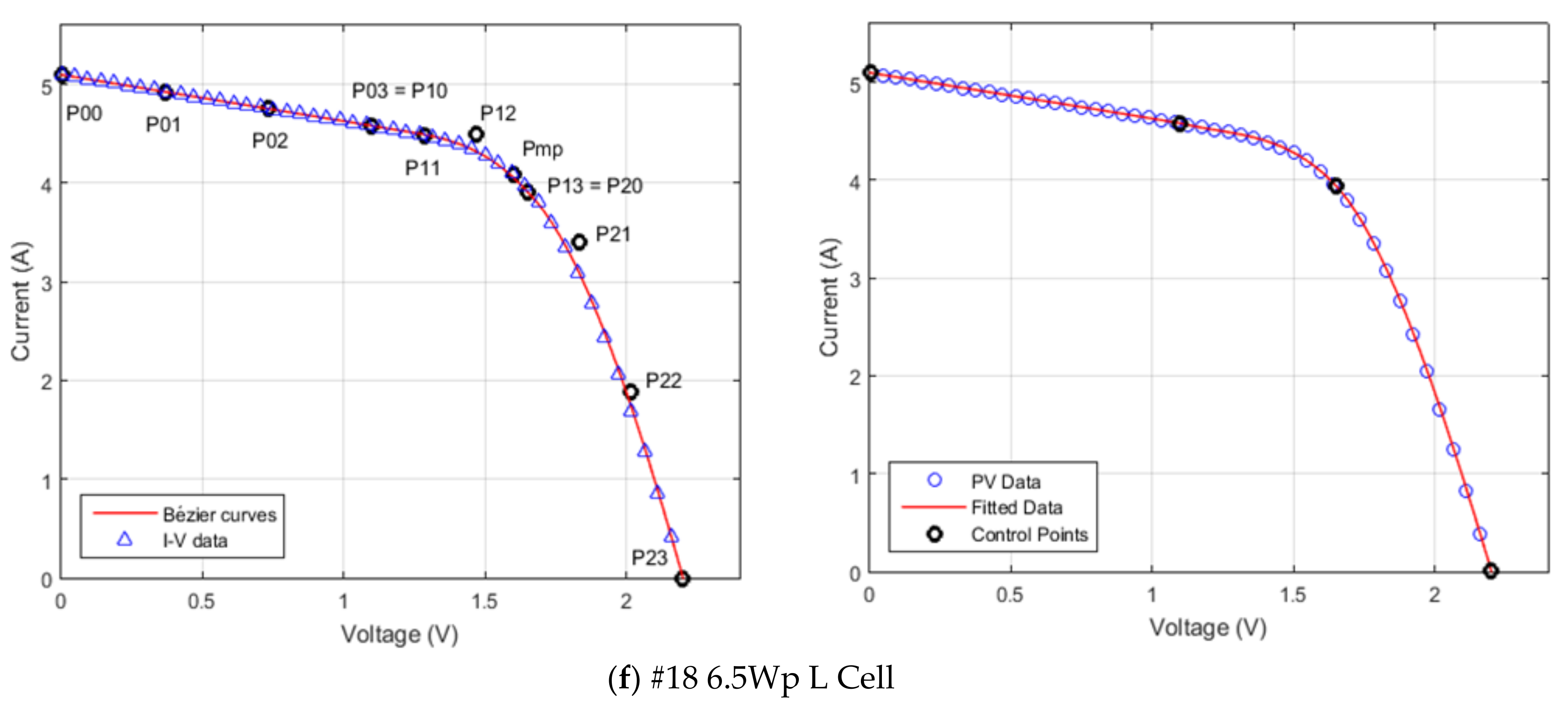
| 18 | 6.5 Wp L Cel | aSi cell | 1 | 2.2 | 1.6 | 4.09 | 5.1 | −0.00836 | 0.00612 |
| No. | |||||||
|---|---|---|---|---|---|---|---|
| 1 | 0.506 | 74.30 | 6.57 × 10⁻¹⁰ | 4.732 | 1.022 | 0.691 | 95.27 |
| 2 | 0.109 | 284.83 | 2.17 × 10⁻⁸ | 8.703 | 1.234 | 0.233 | 304.09 |
| 3 | 0.378 | 220.45 | 2.55 × 10⁻¹⁰ | 8.735 | 1.012 | 0.535 | 266.54 |
| 4 | 0.142 | 192.59 | 5.23 × 10⁻¹⁰ | 8.586 | 1.023 | 0.372 | 202.92 |
| 5 | 0.308 | 193.05 | 2.15 × 10⁻⁹ | 8.223 | 1.076 | 0.463 | 225.66 |
| 6 | 0.277 | 439.46 | 1.63 × 10⁻⁹ | 5.343 | 1.071 | 0.437 | 502.34 |
| 7 | 0.19 | 51.83 | 1.51 × 10⁻⁹ | 8.401 | 1.067 | 0.3161 | 60.474 |
| 8 | 0.28 | 140.26 | 1.56 × 10⁻⁹ | 8.928 | 1.067 | 0.438 | 161.66 |
| 9 | 0.317 | 108.98 | 1.41 × 10⁻⁹ | 8.354 | 1.057 | 0.501 | 127.07 |
| 10 | 0.968 | 1.24E+06 | 3.41 × 10⁻¹⁰ | 2.3 | 1.022 | 1.332 | 151053 |
| 11 | 0.316 | 146.08 | 1.22 × 10⁻⁹ | 3.808 | 1.045 | 0.557 | 164.26 |
| 12 | 0.009 | 4.19 | 1.21 × 10⁻⁹ | 3.809 | 1.045 | 0.016 | 4.788 |
| 13 | 0.264 | 405.65 | 5.50 × 10⁻¹⁰ | 8.686 | 1.030 | 0.458 | 450.79 |
| 14 | 1.555 | 210.33 | 3.30 × 10⁻⁹ | 2.7 | 1.23 | 2.168 | 300.48 |
| 15 | 0.437 | 117.72 | 1.75 × 10⁻¹¹ | 7.397 | 1.058 | 0.637 | 138.19 |
| 16 | 11.57 | 186.22 | 1.21 × 10⁻¹³ | 1.179 | 0.856 | 13.60 | 204.51 |
| 17 | 16.639 | 418.79 | 8.60 × 10⁻¹⁴ | 0.769 | 0.856 | 19.50 | 459.43 |
| 18 | 0.079 | 2.06 | 1.52 × 10⁻⁹ | 5.296 | 3.938 | 0.103 | 2.13 |
| No. | x Coordinates (V) | y Coordinates (A) | |||||||||
|---|---|---|---|---|---|---|---|---|---|---|---|
| 03 | 13 | 00 | 01 | 02 | 03 | 11 | 12 | 13 | 21 | 22 | |
| 1 | 10.628 | 15.931 | 4.732 | 4.684 | 4.637 | 4.588 | 4.538 | 4.606 | 4.360 | 4.212 | 2.575 |
| 2 | 11.295 | 16.930 | 8.703 | 8.690 | 8.678 | 8.663 | 8.635 | 8.696 | 8.508 | 8.210 | 8.125 |
| 3 | 18.870 | 28.285 | 8.735 | 8.706 | 8.678 | 8.649 | 8.604 | 8.697 | 8.453 | 8.529 | 5.997 |
| 4 | 22.224 | 33.312 | 8.586 | 8.547 | 8.509 | 8.470 | 8.443 | 8.453 | 8.370 | 7.684 | 9.991 |
| 5 | 16.425 | 24.620 | 8.223 | 8.194 | 8.167 | 8.137 | 8.094 | 8.178 | 7.930 | 7.909 | 5.930 |
| 6 | 10.845 | 16.256 | 5.343 | 5.335 | 5.327 | 5.318 | 5.298 | 5.350 | 5.212 | 5.200 | 4.168 |
| 7 | 10.975 | 16.451 | 8.401 | 8.3301 | 8.260 | 8.189 | 8.128 | 8.178 | 7.946 | 7.918 | 6.273 |
| 8 | 18.415 | 27.603 | 8.928 | 8.883 | 8.841 | 8.796 | 8.749 | 8.812 | 8.595 | 8.581 | 7.029 |
| 9 | 18.228 | 27.362 | 8.354 | 8.298 | 8.243 | 8.187 | 8.133 | 8.191 | 7.967 | 7.954 | 6.288 |
| 10 | 10.940 | 16.399 | 2.300 | 2.300 | 2.300 | 2.299 | 2.287 | 2.331 | 2.226 | 2.180 | 1.367 |
| 11 | 10.527 | 15.779 | 3.808 | 3.784 | 3.760 | 3.736 | 3.715 | 3.733 | 3.649 | 3.599 | 3.241 |
| 12 | 0.293 | 0.438 | 3.809 | 3.786 | 3.763 | 3.739 | 3.718 | 3.738 | 3.652 | 3.608 | 3.204 |
| 13 | 22.336 | 33.479 | 8.686 | 8.667 | 8.649 | 8.630 | 8.606 | 8.650 | 8.525 | 8.411 | 8.209 |
| 14 | 11.565 | 17.335 | 2.700 | 2.680 | 2.666 | 2.642 | 2.606 | 2.669 | 2.275 | 1.868 | 0.969 |
| 15 | 21.720 | 32.557 | 7.397 | 7.336 | 7.274 | 7.213 | 7.168 | 7.185 | 7.063 | 7.200 | 5.950 |
| 16 | 23.500 | 35.225 | 1.110 | 1.0717 | 1.0343 | 0.995 | 0.971 | 0.978 | 0.775 | 0.578 | 0.289 |
| 17 | 23.500 | 35.225 | 0.740 | 0.723 | 0.707 | 0.689 | 0.677 | 0.686 | 0.542 | 0.403 | 0.201 |
| 18 | 1.100 | 1.649 | 5.100 | 4.928 | 4.760 | 4.584 | 4.456 | 4.506 | 3.949 | 3.372 | 1.786 |
| No. | Current () Error | Max. Power Error | ||||||
|---|---|---|---|---|---|---|---|---|
| Avg.Rel. (%) | Coordinates | Abs. (mA) | Rel. (%) | Abs. (W) | Rel. (%) | Comp. (W) | ||
| (V) | (A) | |||||||
| 1 | −0.11 | 18.423 | 3.247 | 16.63 | 0.52 | −0.363 | −0.52 | 70.32 |
| 2 | −0.08 | 20.398 | 6.325 | 21.97 | 0.35 | −0.246 | −0.16 | 150.47 |
| 3 | −0.21 | 32.952 | 6.615 | 59.85 | 0.90 | −1.80 | −0.74 | 246.90 |
| 4 | 0.10 | 34.638 | 8.319 | 92.81 | 1.12 | −1.99 | −0.66 | 302.10 |
| 5 | −0.19 | 28.788 | 6.183 | 50.70 | 0.82 | −1.223 | −0.61 | 201.37 |
| 6 | −0.20 | 19.077 | 4.105 | 33.65 | 0.82 | −0.481 | −0.55 | 87.83 |
| 7 | −0.20 | 19.306 | 6.225 | 52.58 | 0.84 | −0.227 | −0.17 | 135.28 |
| 8 | −0.20 | 32.432 | 6.801 | 57.57 | 0.85 | −1.242 | −0.51 | 246.50 |
| 9 | −0.20 | 32.103 | 6.248 | 53.40 | 0.86 | −1.308 | −0.58 | 225.75 |
| 10 | −0.13 | 18.548 | 1.675 | 9.200 | 0.55 | −0.240 | −0.67 | 36.21 |
| 11 | −0.17 | 18.697 | 2.867 | 19.97 | 0.70 | −0.215 | −0.36 | 60.07 |
| 12 | −0.17 | 0.519 | 2.872 | 20.60 | 0.72 | −0.006 | −0.38 | 1.669 |
| 13 | −0.17 | 39.909 | 6.788 | 47.91 | 0.71 | −0.914 | −0.30 | 301.49 |
| 14 | 0.03 | 12.255 | 2.635 | 3.32 | 0.13 | 0.093 | 0.23 | 39.91 |
| 15 | −0.27 | 38.253 | 5.730 | 67.47 | 1.18 | −1.253 | −0.52 | 241.59 |
| 16 | 0.04 | 30.966 | 0.925 | 0.94 | 0.10 | 0.015 | 0.05 | 28.79 |
| 17 | 0.04 | 30.816 | 0.650 | 0.79 | 0.12 | 0.010 | 0.05 | 20.15 |
| 18 | 0.014 | 1.578 | 4.142 | 7.09 | 0.17 | 0.01 | 0.16 | 6.53 |
© 2018 by the authors. Licensee MDPI, Basel, Switzerland. This article is an open access article distributed under the terms and conditions of the Creative Commons Attribution (CC BY) license (http://creativecommons.org/licenses/by/4.0/).
Share and Cite
Szabo, R.; Gontean, A. Photovoltaic Cell and Module I-V Characteristic Approximation Using Bézier Curves. Appl. Sci. 2018, 8, 655. https://doi.org/10.3390/app8050655
Szabo R, Gontean A. Photovoltaic Cell and Module I-V Characteristic Approximation Using Bézier Curves. Applied Sciences. 2018; 8(5):655. https://doi.org/10.3390/app8050655
Chicago/Turabian StyleSzabo, Roland, and Aurel Gontean. 2018. "Photovoltaic Cell and Module I-V Characteristic Approximation Using Bézier Curves" Applied Sciences 8, no. 5: 655. https://doi.org/10.3390/app8050655
APA StyleSzabo, R., & Gontean, A. (2018). Photovoltaic Cell and Module I-V Characteristic Approximation Using Bézier Curves. Applied Sciences, 8(5), 655. https://doi.org/10.3390/app8050655