Comparison of Heuristic Algorithms in Discrete Search and Surveillance Tasks Using Aerial Swarms


Centre for Automation and Robotics (CAR), Technical University of Madrid (UPM), 28006 Madrid , Spain
*
Author to whom correspondence should be addressed.
†
Current address: C/ José Gutiérrez Abascal, 2, 28006 Madrid, Spain.
Appl. Sci. 2018, 8(5), 711; https://doi.org/10.3390/app8050711
Submission received: 24 March 2018
/
Revised: 24 April 2018
/
Accepted: 2 May 2018
/
Published: 3 May 2018
(This article belongs to the Special Issue Swarm Robotics)
Abstract
:The search of a given area is one of the most studied tasks in swarm robotics. Different heuristic methods have been studied in the past taking into account the peculiarities of these systems (number of robots, limited communications and sensing and computational capacities). In this work, we introduce a behavioral network made up of different well-known behaviors that act together to achieve a good performance, while adapting to different scenarios. The algorithm is compared with six strategies based on movement patterns in terms of three performance models. For the comparison, four scenario types are considered: plain, with obstacles, with the target location probability distribution and a combination of obstacles and the target location probability distribution. For each scenario type, different variations are considered, such as the number of agents and area size. Results show that although simplistic solutions may be convenient for the simplest scenario type, for the more complex ones, the proposed algorithm achieves better results.
1. Introduction
1.1. Multi-Agent and Swarm Robotics
In nature, as well as in our societies, it is easy to find individuals that act together to achieve a specific goal. In some cases, a good performance cannot be achieved without a coordinated action of various agents. In some other cases, it may be even mandatory to use more than one agent. With the development of robotics, it has been possible to cover increasingly complex tasks by using groups of intelligent agents that coordinately act as a team. In many circumstances, subdividing those tasks not only speeds up their fulfillment, but also allows specialization by allocating specific tasks to agents designed for those purposes. On the other hand, multi-agent systems present important complexities that must be correctly addressed, among which we can highlight the coordination of the agents, the communications between them and how to make the team learn in order to improve the performance.
There are several cases in which the use of multi-agent systems may be desirable. In [1], three types of tasks are considered: tasks that require multiple agents (for example, a task that needs the simultaneous presence of an agent in two places separated by a great distance); tasks that are traditionally multi-agent (e.g., because they can be naturally divided); and tasks that might benefit from the use of multiple agents. Search, surveillance and exploration belong to this last group. Some other tasks might not benefit from the use of more than one robot, either because they are simple or because the development of the coordination and the communication between the members is a barrier not worth overcoming.
Some examples in nature show that individually, simple animals have been capable of surviving during millions of years all over the Earth. Consider for example the most well known of these animals, ants. Ants have a very simple nervous system made up by 250,000 neurons and very limited sensing and communication capabilities. Communications are achieved mostly by pheromones [2], chemicals spread in the environment used to mark trails, warn other members of the nest and confuse enemies. It is obvious how difficult it would be for them if they had to survive individually. However, acting as a coordinated group, they have survived for 130 million years and form around 15–25% of the terrestrial animal biomass. The reason why such a simple creature has been so successful is because of their collective behavior. Every ant acts in a very simple way that turns out to be very inefficient individually. However, collectively, because of the high number of members, an efficient behavior emerges. Similar social structures and interactions may be found in other species, such as bees, termites, fishes (forming schools), ungulates and birds (flocks).
Swarm behaviors are a particular case of collective behavior, in which a large number of members is involved, requiring very limited communications between them and being individually simple. Some researches started bringing the ideas of swarms in nature to the robotics field. Goals are achieved using a high number of homogeneous robots, which behave following simple and mostly reactive rules. The pioneers of swarm robotics appeared in the late 1980s and the beginning of the 1990s [3,4,5]. Swarm robotic systems present some well-known advantages such as robustness, simplicity, scalability and flexibility, while it is difficult to achieve a good global performance [6]. More recently, many researchers have used the term swarm robotics to name or classify these works. Hardware miniaturization and cost reduction have made possible new research lines in this direction, and hundreds of papers developing all sorts of algorithms have been published.
1.2. Search with Swarms
From the very beginning of the development of swarm robotics, researches have focused on implementing behaviors in robots to solve simple tasks [7]. Those behaviors are mainly inspired by how natural swarms act, and the missions may be used as test beds for more complex and useful tasks. Typical examples of them are aggregation (gathering in a common place), flocking, foraging (collecting items scattered in the space), path formation (establishing a path of robots between two points) and deployment (expanding and occupying the available space). Note that all of these behaviors are very common in animal swarms such as fish schools, bird flocks, ants and bees.
Besides those basic tasks, more complex missions have been also studied in the past. Exploration of unknown areas, search, surveillance, patrolling, collaborative manipulation and self-assembly are only some examples of missions that have been carried out with robotic swarms. In this work, the focus is on the search task, where multiple and different solutions have been proposed over the years. Most of these methods may be assigned to one of the following categories:
As can be seen, all the previous solutions are heuristic methods, since they do not guarantee optimal solutions. There have been approaches trying to optimally solve the search, although they require high computational loads, and the calculations only reach reduced time horizons. Note that the number of solutions increase exponentially with the number of agents, making the finding of optimal solutions almost intractable. Some of these methods will be briefly reviewed in Section 1.4.
In this paper, we propose an algorithm based on a behavioral network, made up by different behaviors that act together to obtain a common decision in order to lead each agent. On the one hand, this type of control responds quickly to changes in the environment (which is a typical property of reactive systems). On the other hand, the behaviors are capable of constructing representations of the world (they have memory, a typical property of the deliberative controls). Decisions are taken as a result of the interactions between the behaviors and the environment and between the behaviors. All this results in a good trade-off between reactive and mid-term decisions [17]. Behavior-based architectures turn out to be adequate for changing and stochastic environments, and therefore, they are also very suitable for multi-agent systems. Note that if each agent makes its own decisions (there is no central planning), the state of the task changes rapidly, and planning at the individual level becomes likely unfeasible.
The search task is an interesting challenge not only because of its direct application in real-world situations, but also because it may be extended to similar, but more complex tasks such as surveillance, exploration, patrolling, area coverage and the so-called traveling salesman problem:
- Exploration: This differs from search in that there does not exist a previous map of the area.
- Surveillance: This is basically persistently searching a given area. Each zone must be re-visited frequently enough to ensure up-to-date information.
- Patrolling: Similar to surveillance, the area of interest is restricted to singular points or lines (for instance, corridors inside a building).
- Probabilistic maps and obstacles: Another extension of the search task in its simplest form is the inclusion of probabilistic maps, which consider prior knowledge about where it is more likely that a target is located in the area. Moreover, obstacles may be included, it being impossible for the agents to go through them.
Authors frequently define area coverage as deploying the agents until they reach certain fixed positions so that the covered area (by either the sensor or the communication footprint) is maximized. However, some other authors use the word coverage to define a task similar to search. For instance, in [18], the search area is covered by subdividing it into k regions, which are individually assigned to k robots. Each robot searches then in its assigned area following regular patterns. Another example can be found in [19], where the coverage task is addressed using the spanning tree coverage method. In any case, the strategies proposed in these works do not differ from the strategies listed above.
1.3. Search Patterns
In order to organize the search, most of the past works based on patterns have made use of dividing the area into cells, taking into account if they have been visited or not. The sensed area is frequently restricted to those cells, and therefore, the search implies visiting all the existing cells. The agent’s movement is restricted, and they are only allowed to travel between the centers of adjacent cells. With these assumptions, the search is simplified since it becomes a discrete problem. In the following, the main works addressing this kind of mission by implementing movement patterns are analyzed.
In [20], the task is addressed with an algorithm made up by four behaviors that act together:
- Contour following: This leads the agent along boundaries, i.e., cells that have at least one non-visited cell surrounding them. This is the behavior with the highest priority.
- Avoidance: When two agents are within a given range, this behavior is triggered. The velocity command is perpendicular to their mutual collision course, and it is added to the contour following the behavior output.
- Gradient descend: Having defined a distance field, computed at each cell as the distance to the closest non-visited cell, when this behavior is active, it leads the agent along the gradient. It is activated when an agent is completely surrounded by visited cells.
- Random movement: The agent decides randomly which cell to visit next. It is activated when none of the other behaviors are active.
The distance matrix is treated here as a pheromone field. The members of the swarm share information with the agents within a communication range, updating the distance matrix (i.e., which cells have been visited). Assuming a constant velocity and considering that traveling diagonally requires the same time as traveling in the other directions, the minimum needed time is then , where is the number of cells and l is the number of agents. The algorithm is tested for different numbers of agents, as well as for different avoidance and communication ranges. The needed time to accomplish the mission is used as the performance measurement. The influence of implementing a central communication point, which distributes the state of the search grid among the agents, is analyzed. Having distributed the agents randomly, the results show that the time needed to finish the mission is higher than the theoretical lower bound, even with the centralization of the information. However, even with short communication ranges, the overtime to complete the search is less than 50%, with a standard deviation of 6% on average due to the variability in the initial conditions. With only one agent, the time needed is close to the minimum bound. Furthermore, another performance measurement criterion is proposed:
where are the number of cells visited more than once and N is the total number of cells. Again, for only one member, this ratio is close to one, whereas for the higher number of agents, this figure decreases. If the communication range increases, the solution converges to the centralized map, as expected.
In another work [21], three search strategies are compared in a mission in which the agents are deployed in an area that contains targets to be localized and destroyed, forming coalitions. The three studied strategies are:
- Random search: Each agent follows its current heading until one boundary is reached. At that moment, it changes its direction to re-enter the search area.
- Search lanes: The area is organized into lanes, and each agent is assigned to a unique one. Once a lane has been traveled, a new one is assigned.
- Grid-based search: The agents go to the closest non-visited cell.
Since in this work, targets to be destroyed are considered, the search task stops to pursue and destroy them. Therefore, no absolute search performance metric is provided, and these behaviors are compared by only considering the time needed to complete the mission. Monte Carlo simulations are run varying the number of agents and targets.
There have been many works in which the task is solved by partitioning the area and assigning individually those partitions to the agents. For instance, in [22], each partition is filled with zig-zag lanes, computed to be energetically efficient. However, the algorithm requires that the area is a polygon on whose boundaries the UAVs must be initially placed, restricting the initial positions.
Making use of the probability that a target is located in a specific cell in [23], scores are assigned to each one, taking also into account forbidden flying zones and areas that should be avoided if possible. The scores are updated either externally or because of the findings of the agents. The agents select the cell to visit depending on that score. In this work, the area is partitioned using a Voronoi diagram, and the results are compared with other algorithms:
- Lawn mower: Each agent moves in a straight line, and when it encounters an obstacle, it turns to head in a clear direction.
- Raster scan: The agents move in parallel lanes north/south or east/west.
- Gradient climb: This is a greedy algorithm based on the surrounding cell scores.
- Randomized Voronoi: The area is partitioned with the Voronoi diagram using the agent’s position as the generators.
- Full algorithm: This is the same algorithm, developed in previous works, but without the Voronoi partitioning.
The algorithms are compared using as a performance measurement the mean cell scores, computed along 20 runs, the most efficient algorithm being the one proposed in the work. This result seems reasonable, since the performance is measured using the same score on which the algorithm is based.
1.4. Optimal Methods in Discrete Search Tasks
Although the discrete search task using teams of agents has been shown to be a hard problem to solve optimally, there have been some works addressing the problem by looking for optimal solutions. For instance, in [24], an exact mixed-integer linear programing formulation to solve in an optimal way the search of a discretized area is proposed. Given a mission state defined by the position of the agents and the cells already visited, the best sequence of movements is calculated for a specific time horizon. While the found path is being followed, a new sequence is generated over a receding horizon. Eight possible movements are considered at each decision instant, as well as a prior belief about where the targets are possibly located. The authors remark that the number of possible solutions for n agents and a time horizon of T movements is , which reaches prohibitive values quickly. Using a six-core processor, for a grid of 10 × 10 cells and considering two and five agents, with time horizons of 10 and 20 steps, optimal solutions are found within one minute (except for one of the cases studied, which needed 142 s). Bigger scenarios and/or more agents are unfeasible to solve.
In [25], a receding time horizon is also used to optimize on-line the trajectories of a group of UAVs in a discrete bi-dimensional search area. Based on the current state of the agents, the optimizer tries to maximize the reward of finding a target and of exploring the area, while it keeps the energy consumption low. The optimization problem is broken down into local ones assuming communications between the agents, so that it can be solved in a decentralized way. For this procedure, Nash optimality is considered and a particle swarm optimization used as the optimizer tool. Simulations are carried out in a search area of 50 km × 50 km (a grid of 500 × 500 units), and the results show that although the decentralized optimization does not reach the performance of the centralized one, it requires half of the computational time.
1.5. Organization of This Paper
This paper is organized as follows: In Section 2, the problem is presented, defining the search area and its grid, the agent’s dynamics and the measurement of the algorithms’ performance. Furthermore, the four different types of scenarios used to compare the algorithms are shown; in Section 3, the proposed algorithm based on a set of behaviors is explained in detail, as well as how it is configured for any scenario. In Section 5, the algorithms are compared measuring their performance for the four scenarios types; also, the communications needed by each algorithm and their adaptation to surveillance missions are analyzed. Finally, in Section 6, the conclusions of this work are depicted, as well as the proposed future developments.
The main contributions of this papers are: (i) the proposal of a behavioral network made up by six behaviors; (ii) systematical comparison with six search patterns in four different scenario types, considering the wide variations of the parameters that define each scenario; (iii) a performance model for this type of mission.
2. Problem Formulation
2.1. Scenario
The task proposed consists of observing a given two-dimensional search space, which is a rectangular area subdivided into cells of fixed size. The movement of the agents is restricted to those cells, so that each agent is allowed to move from the center of each cell to the center of any of the eight adjacent cells. As already mentioned, this assumption is convenient, since it converts the search into a discrete problem, simplifying it.
We consider that the search is carried out by flying robots, more specifically, multicopters. The agents are capable of flying at a constant altitude and at given commanded velocity and are equipped with a camera capable of detecting targets within a circular area of radius . This area is called the sensor footprint. The team of robots is made up by of equal multicopters, initially deployed randomly in non-coincident positions in the search area. Each agent will be configured equally, i.e., the control parameters will be the same for each one.
Having divided the search space into a grid, with a total area of (m), we allow the robots to move to any adjacent cell. In order to ensure that the cells are completely observed by the sensor footprint, they must be inscribed in it. Therefore, the number of cells in each direction is:
where indicates the ceil function, and the dimensions of each search cell are:
When flying in any direction, part of the adjacent cells is observed; see Figure 1. Those cells, which we will denominate from now on search cells, should be then subdivided into thinner cells to take into account whether those portions of space have been observed or not. We will refer to these other cells as discretization cells. Therefore, the movement will be restricted to the search cells, but not the search task itself, since a search cell can be completely observed without visiting it. We consider for the rest of the work a size of the discretization cells of 2 × 2 m, i.e., .
In Figure 1, both types of cells have been represented. We define observing a cell as placing an agent so that at least half of that discretization cell is inside the sensor footprint. We also define visiting a cell as placing an agent in the center of that search cell. Since the search cells are inscribed in the sensor footprint, visiting a search cell implies observing the discretization cells inside it.
In Table 1, the parameters that define the scenarios with their considered range of values have been presented. Note that instead of limiting the total search area , it is more sensible to limit the search area per agent, . On the other hand, we define the aspect ratio of the search space as:
2.2. Plain, Obstacles and Probability Scenarios
Given the scenario above described, four different types of scenarios are considered:
- Plain scenario: In the simplest scenario type, every cell is flyable, and all the discretization cells must be observed at least once to finish the mission (see Figure 2a).
- Probability distribution scenario: We assume prior knowledge about the possible location of targets to be found. According to this distribution, targets are generated. The search is finished when all the targets have been observed. The probability distribution is generated using the midpoint displacement method, normally used as a terrain generator method. The initial distribution is generated randomly with a roughness and its derivative . Seven iterations are applied. In Figure 2b, an example of this scenario type is shown.
- Obstacles scenario: Some of the search cells are occupied, and the agents cannot fly through them. The search is completed when all the discrete cells that are not inside the obstacles have been observed at least once. The map is generated using the Schelling segregation model, fixing the tolerance limit to 0.3 and the percentage of the population that look for new houses to 0.7. The percentage of non-flyable search cells is drawn from a normal distribution , while the percentage of empty cells (cells that may be occupied by obstacles) is drawn from . Once the equilibrium has been reached, the empty cells are transformed into flyable cells. It is checked that every flyable cell can be reached (i.e., there are no cells completely surrounded by obstacles). An example of the result of this procedure has been shown in Figure 2c.
- Probability distribution and obstacles scenario: Both the probability distribution of target locations and obstacles are considered; see Figure 2d.
2.3. Model of the Agent
2.3.1. Dynamics
The agent considered here is a multicopter, i.e., a holonomic UAV capable of flying in any direction and keeping a fixed position. The high level control generates a commanded velocity in the plane, defined by two variables, a reference velocity and its heading . The actual velocity vector is modeled as:
where is assumed to be dependent on the change of the flying direction:
where is the time instant at which the agent changes its direction and is the characteristic time for the velocity reduction due to the change in the flying direction ().
2.3.2. Energy Consumption
The agents are considered to have an energy consumption proportionally to the flown distance:
where is the dimensionless energy needed to fly a distance d (m) and is a coefficient. Furthermore, if a quadcopter changes its flying direction, an extra energy consumption is considered:
where is the dimensionless energy needed to change the flying direction in radians and is a coefficient. The remaining energy in each quadcopter will be then calculated as:
being the maximum energy in the quadcopter’s batteries. In Table 2, the chosen values for the parameters that define the model have been presented.
2.4. Measuring the Performance
As already seen, in past works, several different ways of measuring the performance of a search task have been proposed. Some of them are not absolute metrics, i.e., they have been created ad hoc for specific missions or situations and cannot be translated in a general way to other search missions. The best way to measure the efficiency would be comparing the performance with a solution whose optimality is ensured. However, as we have seen, only partial optimal solutions (with limited time horizons) have been achieved. Therefore, we will make use of three different models or methods to measure the efficiency.
2.4.1. Model 1
The first model we consider is the one presented in [23]. The efficiency is measured with a coefficient between the total number of search cells and the number of search cells that have been visited more than once:
where is the number of search cells visited more than once and N is the total number of search cells. Note that if every cell is visited only once, the efficiency reaches the maximum value, equal to one.
2.4.2. Model 2
In the first model of the efficiency, the search cells have been considered to measure it, counting whether they have been visited more than once or not. However, when traveling diagonally, parts of the surrounding cells are observed, as well. In order to take this into account, in this second model, Equation (10) is used, but considering the discretization cells:
being the discretization cells that have been observed more than once and n the total number of discretization cells. With this approach, a result closer to the reality is expected.
2.4.3. Model 3
A final third model of the efficiency is proposed, and it is based on the time the team of agents need to complete the search. The ideal performance would be reached if the search area was completely observed without observing any of the discretization cells more than once and if during the search process, no part of the agent’s footprint is outside the search area. If this were the case, the time needed to observe a specific area would be:
where is the observed area at and is the actual observed area at the end of the mission. Note that in some missions, depending on the search area per agent, the footprint sensor radius and the configuration of the algorithm, it may be if the available energy is limited. If this is the case, we consider that the search is not completed. If a group of agents needs a time to completely observe that area, we can define the efficiency as:
where . Note that reaching an efficiency equal to one, i.e., , is not possible since the footprint invades part of the adjacent cells, and therefore, when flying over the cells at the boundaries, part of the sensor footprint would be outside the search area, implying a loss of efficiency. It is also very likely that some of the discretization cells are observed more than once. Probably if we chose the search cells so that the footprint is inscribed inside them, the efficiency would increase. However, the corners of the search area would never be observed.
2.4.4. Fitness Function
In Section 2.3.2, we have assumed that each agent accounts for a specific amount of available energy; once it is consumed, it stops flying, and therefore, it stops observing the scenario. Depending on how efficient the configuration of the algorithm is and on the scenario characteristics, it may happen that the search area is not completely observed. In those cases, the efficiency will be penalized by only considering 25% of the efficiency. Note that it may happen that for the same scenario, with the same configuration of the algorithm, the task may be completed or not depending on the initial conditions. In those cases, the efficiency penalization will be only applied for the trials in which the search has not been completed.
We assume that the efficiency depends on the initial conditions, for a given configuration and scenario . We consider that a configuration is robust if for different initial conditions, it achieves efficiencies with a small standard deviation, since it is capable of carrying out the task within similar periods of time, independently of the initial positions. Therefore, instead of evaluating the goodness of the configuration with the efficiency, we define a fitness function that accounts for this:
where is a correction factor that penalizes high standard deviations, being ; is the penalization in the case that the search is not completed. Based on experience, it has been chosen , considering this value as reachable if the algorithm is properly configured. In Figure 3, the correction factor has been represented for as a function of the standard deviation.
3. Proposed Search Algorithm, a Set of Behaviors: A1
3.1. Search Behavior
This first behavior is the main one and leads the multicopter to search unexplored areas. It is based on the presence of virtual pheromones, whose dynamics and different classes are explained in the next subsections. The virtual pheromones are created on the search space and are absorbed by the robots as the area is observed. The robots are then attracted to unobserved zones, where the concentration of the pheromones is higher.
3.1.1. Pheromone Dynamics
The dynamics of the virtual pheromones have been implemented following the bi-dimensional heat flow (or gas diffusion) equation:
where is the concentration of the virtual pheromones, ∇ is the divergence operator, is the pheromone flux and D is the diffusion coefficient and represents how well the pheromones are transported. S is the source of pheromones, i.e., the creation of pheromones at each discretization cell.
Using the divergence theorem in Equation (15) and considering as volumes of control the discretization cells, we can solve the obtained integral equation with an explicit scheme, forward in time and centered in space (FTCS). We consider therefore mean values of and S inside those cells and mean values of and D along their boundaries. The problem is then properly posed by finally defining the initial and the boundary conditions:
The first equation represents the initial concentration of pheromones over the search space, whereas the next four are von Neumann conditions, which state that the pheromone’s flux through the boundaries must always be zero. Obstacles inside the scenario are impermeable to the pheromones flux, similarly to the boundaries of the area.
3.1.2. Cell Types and Properties
The properties of each discretization cell, i.e., the concentration, creation and diffusion of pheromones, variables , and associated with the cell at moment k, depend on three types of cells:
- Non-observed cells: cells that have not been observed yet:
- Observed cells: cells already observed by any agent:
- Recently-observed cells: if a cell has just been observed, there is n instantaneous drop of its pheromone concentration of:where indicates variation due to the fact that the cell has recently been observed and . This drop is accounted only once, so that at the next time step, a recently-visited cell becomes a regularly-visited cell.
- Isolated cells: Each non-observed cell has associated a so-called isolation index, , which is the number of observed cells surrounding it. If the cell has already been observed, its isolating index is forced to be equal to zero. Every time step the isolation index changes, there is an increment in the pheromone concentration of:where is the variation of the isolation index from time k to :The parameter makes the concentration increase when its isolation index changes. Moreover, there is an extra pheromone creation proportional to the isolation index in these cells:
In Figure 4, the above-mentioned cells have been represented. The white discretization cells have not been observed yet. At each time step, the cells that have just been observed become recently-observed cells, in dark green. In the next step, those cells become regular observed cells, in light green. Note that even though there may be a variation in the isolation index at position , the variation of the isolation index is forced to be zero, since the cell becomes observed. In the example shown in the figure, the pheromone concentration in those four cells will suffer a variation, exclusively due to the type of the cell (), of:
Besides these changes in the concentration of pheromones, the natural diffusion, Equation (15), will also apply during each time step.
If there is a prior probability distribution of the possible location of the targets, it can be easily implemented in the algorithm. Given a probability distribution , each discretization cell is assigned a probability value :
being therefore:
and this probability distribution is finally normalized with the maximum value:
and therefore, . The sources of pheromones, as well as the initial value of the pheromones (see Equations (15a) and (16a)) are then multiplied by the associated normalized probability . In this way, the regions where it is more probable to find a target generate more pheromones, and the agents are more attracted to them.
3.1.3. Layers of Pheromones
The actual usefulness of pheromones is to transmit information about observed and non-observed cells along the search area, so that the agents are aimed at zones with more unobserved cells. This way, it is expected that the observed cells generate and transmit less pheromone levels than the unobserved ones. However, if there exist unobserved cells, surrounded by observed cells, it is possible that these last ones act like a barrier, avoiding an effective transmission of the information by the pheromones. On the other hand, it is our experience that it is useful to try to organize the search by prioritizing the observation of isolated (i.e., with high values) cells surrounding each agent. In order to address these issues, we propose a multi-layer pheromone system made up by three independent layers:
- Standard layer (L1): There is no impact of the isolation index on this layer, and it has different diffusion coefficients for observed and unobserved cells.
- Long-range layer (L2): Intended to transmit information from unobserved cells along the entire search area. The diffusion coefficients of observed and unobserved cells are equal, and the observed cells do not produce pheromones.
- Isolation layer (L3): This mainly considers pheromone creation due to the isolation index. Once the cells are observed, they lose their pheromone concentration at this layer.
In Table 3, the parameters for the three layers are summarized. Each parameter has been named with a super-index to indicate the layer to which they belong, except for and , which only apply to Layer 3.
3.1.4. Evaluating Modes
Each time an agent reaches the center of a search cell, it makes the decision of which search cell to visit next, and the search behavior will be taken into account, depending on the concentration of pheromones on the surrounding cells at each layer.
At each time step, each discretization cell has associated a concentration of pheromones at each layer l. The total quantity of the pheromones concentration is then:
Each search cell has associated a set of discretization cells, so that their centers lie inside it. Furthermore, if the final search cell g is in a diagonal position (with respect to the agent), half of the contiguous cells will be observed (see Figure 1), and therefore, the discretization cells inside these halves will be accounted for.
We propose two methods for accounting for the pheromone level at each search cell, for candidates to be visited next:
- Mean values: The mean values of the pheromone concentration of the cells inside each search cell are considered. The income for each surrounding cell is then calculated:
- Maximum values: The maximum value of the concentration inside each search cell is considered.
To consider both solutions, the total income of each surrounding cell g will be calculated as a weighted sum of both:
where is the weighting parameter, to be set.
3.2. Energy Saving Behavior
As already mentioned in Section 2.3.2, there is a need for extra energy to change the direction of flight, besides the energy needed to continue flying. This increment in the consumption depends on how much the direction of flight changes. Moreover, there is a reduction of velocity when the agent changes its flight direction (see Equation (6)), which will have an impact on the performance. In Figure 5a, the energy costs for each cell g considered has been shown. As we will see, since those values will be multiplied by a coefficient, their absolute values are not relevant, but only the relationship between them.
3.3. Diagonal Movement Behavior
Moving in the diagonal might improve the performance of the search since there is potentially less overlap between the sensor footprints. Therefore, a behavior is proposed to encourage the movement in these directions, equal to the pheromone concentration in those cells:
where is the Dirac delta centered in each diagonal cell and is the input due to the pheromone concentration; see Equation (30).
3.4. Collision Avoidance Behavior
To avoid collisions between the agents, this behavior is considered. Every time an agent makes the decision about which cell to visit next, it advises the other agents.
It is important to remark that this behavior does not prevent the collision itself, since two agents may head to two different cells and collide anyway. However, this is an assumed simplification, considering that there will be also a collision avoidance system to take over the control in those situations. The cost of is considered; see Figure 5b.
3.5. Keep Distance Behavior
Imitating several animal species in nature, such as bird flocks, fish schools and ungulate herds, this behavior is proposed. Each agent tries to keep a stable distance with the surrounding agents, by means of the result of attractive and repulsive forces. These are normally implemented similarly to the attractive-repulsive forces presented in the molecules’ interactions. The total force over an agent i due to the presence of an agent j is made up of two forces:
where is the attractive force, is the repulsive force and is the vector from the position of agent i to the position of agent j, . , and are parameters to be set.
Since the configuration is expected to be valid no matter how many agents are carrying out the task or the size of the search area, it is convenient to adimensionalize the distance . There are two candidates for this purpose, the footprint radius:
and a distance representing the size of the search area:
If one takes the first option, the keep distance behavior will be related to the covered area at each moment, and it will lead the agents to behave more as a flock. On the other hand, if the second option is chosen, the agents will tend to cover bigger zones, spreading out themselves across the search area. In order to let the optimization choose any combination of these characteristic distances, a weighted distance is considered:
where is a coefficient to be chosen. The adimensionalized distance is then obtained by:
Making in Equation (32), we get the equilibrium distance, whereas differentiating that equation and equaling it to zero, we get the distance at which the attractive force is maximum:
where . To reduce the number of parameters, we consider, as well:
so that Equation (37a) becomes:
With this assumption, we finally get the relationship:
Again, since this behavior will be multiplied by a coefficient, the actual value of the total force is irrelevant, and therefore, we can take . The behavior so posed depends only on three variables, the adimensionalized distance at which the forces are at equilibrium, , the adimensionalized distance at which the attractive force is maximum, , and the characteristic distance, . Once these distances are set, and are calculated with Equations (40a) and (38), respectively. is calculated with Equation (40b), and finally, with Equation (39), we get . In Figure 6a, the resultant forces have been represented for and . Having the number of agents, the total force on agent i will be:
Once the total force vector over an agent has been calculated, an income value must be assigned to each surrounding cell. Given the direction of and its modulus , a normal distribution is used along the different headings of the surrounding cells:
where is the income corresponding to the surrounding cell g, is the variance of the normal distribution, and it has been chosen as ; is the difference of the heading of and the heading of each surrounding cell g. In Figure 5c, an example of the keep distance behavior has been represented. Agents 2 and 3 apply two repulsive forces and on Agent 1. The total force in this example is . The incomes for each surrounding cell have been calculated with Equation (42). In this case, since the heading of the total force is , we have:
3.6. Keep Velocity Behavior
Similar to the keep distance behavior, and mimicking flocks and schools, a behavior aimed at keeping the velocity of the other agents is also implemented. Most of these sorts of behaviors are proportional to a certain function of the distance between the agents; see, for instance, [26]. Here, a similar law is proposed. The total velocity effect over an agent i is calculated as:
where is the velocity vector of agent j, different from agent i, and is a function of the distance between both agents:
where is the adimensional distance between agents i and j and is the coefficient to be configured. In this case, the characteristic distance is taken equal to the sensor footprint:
In Figure 6b, the function , Equation (45), has been represented depending on the adimensional distance for three values of . Once the total velocity over agent i has been calculated, the incomes of each surrounding cell are calculated similarly to Equation (42):
where and . An example of incomes for each cell has been presented in Figure 6b, where it has been assumed m/s.
3.7. Final Decision
Once every income for each behavior has been calculated, a final decision process takes place. For each surrounding cell g, a final decision income is calculated as follows:
where is the total income of cell g, is the income due to the pheromone concentration, is the energy cost, is the income due to the diagonal movement behavior, is the collision cost, is the income due to the keep distance behavior and is finally the income due to the keep velocity behavior. Note that the above Equation (48) is a weighted linear sum of all costs and incomes, where , , and are the weights to be set. The next cell to visit is then chosen so that the total income is maximum.
3.8. Configuration of the Algorithm
As we have shown, the algorithm consists of six different behaviors with a total of 23 parameters to be selected. Moreover, the optimum values of these parameters presumably depend on the scenario, i.e., on the values of the variables shown in Table 1. To solve this optimization problem, the following procedure was carried out.
Given any plain scenario i (the scenario shown in Figure 2a) defined by the tuple , the algorithm parameters must be configured accordantly to achieve an appropriate performance. If we have a big-enough dataset of scenarios with N suboptimal configurations , i.e., with N suboptimal values for each of the 23 parameters of the algorithm, we can model them individually as a function of the scenario, using as predictors. As a result, for any scenario , a suboptimal estimation is obtained, and the algorithm can then configured. The model selected to predict the suboptimal values is a Gaussian process (see [27]). To generate the dataset of suboptimal configurations, a genetic algorithm is used, whose main characteristics are:
- Chain of genes: a vector made up by the 23 parameters of the algorithm. Each of the genes is normalized with a range of possible values.
- Population: 100 members.
- Initial population: Half of the initial population is taken from the two closest scenarios already optimized, 25 from each one. To select those members, a trade-off between fitness and genetic diversity is considered. The other half is taken as a prediction of the model. Since the model is probabilistic, these 50 member are drawn from the normal distribution of the Gaussian process.
- Fitness function: To evaluate each member, Equation (14) is used. In order to measure the noise due to the variability of the initial conditions, each member is tested 100 times.
- Crossover: The members will be combined using the roulette-wheel technique, with a probability proportional to the fitness value. Two pairs made up by the same two members is forbidden. Two members being selected for the crossover, a new member will be created by applying a weighted sum of each gene individually. The weighting coefficient is a random number between zero and one. The offspring is made up of 50 new individuals.
- Next generation selection: After evaluating the new individuals, elitism is used to select the 100 best members for the next generation from the 150 available members.
- Stopping criteria: The optimization is stopped when one of these criteria is met:
- –
- Maximum number of generations (30) has been reached.
- –
- Maximum time for each optimization (24 h) has been reached.
- –
- Maximum number of generations (10) without an improvement higher than 10% of the best member has been reached.
- –
- Maximum number of generations (3) without an improvement higher than 10% of the mean fitness of the population has been reached.
Having obtained suboptimal configurations for k scenarios, the next scenario is obtained so that the mean uncertainty of the GPs of the 23 parameters is most reduced, i.e., the scenario with the highest uncertainty is selected. A total of scenarios is optimized and used as the dataset. In Figure 7, the complete modeling process has been schematically depicted.
4. Search Patterns
In this section, six search patterns are proposed, which will be compared with the above explained set of behaviors.
4.1. Random Walk: A2
The simplest solution to explore the area is to walk randomly. Every time an agent reaches the center of a search cell, it randomly decides which surrounding cell to visit next. Given a present heading , the next course will be then , being:
where indicates normal distribution and is its standard deviation, which has been chosen as . Since the movement is restricted to the surrounding eight cells, is rounded to the closest possible heading pointing to any of those cells. In addition to this behavior, the collision avoidance is also implemented as explained in Section 3.4. In Figure 8, an example of a random walk has been represented for two agents.
4.2. Go to the Closest Non-Visited Cell: A3
The next pattern to be compared is heading to the closest cell that has not been already visited. The distance is computed as the Euclidean norm, and once the target cell is selected, the needed heading is obtained. Depending on that course, utility values are assigned to the surrounding cells as per:
where it has been chosen . Note that this utility assignment is similar to the one used in the keep distance and keep velocity behaviors; see Equations (42) and (48). If there is more than one cell at the same distance, the utilities for each surrounding cell are calculated and summed up. In addition to this behavior, the energy saving and the collision behaviors are implemented; see Section 3.2 and Section 3.4. This implies that if more than one cell is situated at a similar Euclidean distance, the agent will head to the one that implies lower energy consumption. The utility of each surrounding cell g is therefore calculated as:
where is the energy cost. In Figure 9, an example of this algorithm has been represented.
4.3. Boundary Following: A4
As proposed in [20], an effective way of traveling along the search area is selecting the next cell to visit depending on if they are surrounded by already-visited cells or not. This way, the task is organized in a compact way.
In order to implement such a behavior, we make use of the isolation index as defined in Section 3.1.2, but instead of applying it on the discretization cells, it will be referred to as the search cells. Each surrounding cell will have a utility equal to its isolation index. Moreover, the energy saving behavior is also implemented, so that for equally-isolated cells, the one that needs less energy is preferred. The utility of each surrounding cell g is therefore calculated as:
Finally, if there is not any surrounding unvisited cell, the behavior go to closest non-visited cell takes over the control. In Figure 10, an example of this behavior has been shown.
4.4. Energy Saving: A5
The energy saving behavior, depicted in Section 3.2, can be implemented separately so that each agent keeps its current course unless a collision may take place, or in case the agent is going to fly outside the search area. In those cases, the safe heading that requires less energy is chosen. In Figure 11, an example of this behavior is represented.
4.5. Billiard Random Movement: A6
Similarly to the lawn mower behavior proposed in [23], the billiard random movement behavior directs the agents to go straight until they encounter any border. Then, they select randomly any other free direction. This behavior differs from the energy saving in the way the next course is selected (randomly here, the most energy convenient in the other). The collision avoidance behavior is also active in this algorithm. In Figure 12, an example of this behavior is shown.
4.6. Lanes Following: A7
Finally, the lanes following algorithm is considered. Similar to the raster scan behavior depicted in [23], a lane is assigned for each agent. The direction of the lanes (north-south or east-west) is selected so that the minimum number of lanes is created; if that number is lower than the number of agents, the other direction is selected. When a lane is assigned to an agent, it goes first to the closest extreme cell of the lane, and after, it starts traveling along it. When the lane is completely observed, the closest non-observed lane is assigned. If there are no available lanes, the go to closest unvisited cell behavior is activated. In Figure 13, an example of this behavior is shown.
5. Comparison of the Algorithms
In order to compare all the search algorithms considered in this work, random scenarios are generated considering the parameters (and their valid ranges) shown in Table 1 for each of the four scenario types. Recall that each scenario is defined by the area per agent, , the number of agents, , the nominal velocity of the robots, , the sensor footprint radius, , and the aspect ratio of the area, . For each scenario, 100 different initial conditions are generated, and each algorithm is tested having considered them. The mean values of the efficiencies as per Models 1, 2 and 3 (see Equations (10), (11) and (13)) are calculated and considering the standard deviations among the 100 trials, the fitness value is obtained according to Equation (14). For this last figure, whether the search has been completed or not is also taken into account.
First, we carry out a quantitative comparison based on the measurement of the efficiency and fitness values for each scenario type. Secondly, we present a qualitative analysis discussing the complexity of the communications needed and how appropriate each algorithm could be for a surveillance mission.
5.1. Quantitative Comparison
5.1.1. Plain Scenarios
In Table 4, the results of the simulations have been presented for the plain scenario. For each of the three models, the mean efficiency among 200 scenarios and the mean fitness value are shown. Notice that in turn for each of the scenarios, the efficiency and the fitness is the result of the mean of 100 trials.
For Model 1, the best algorithms turn out to be A4, A3, A7 and A1, with an efficiency between 70 and 78%. In any case, the efficiencies of all algorithms lie above 78% of the maximum efficiency (0.61/0.78 = 0.78), which may indicate a bad representation of the real performance of the algorithm. Note that even a random movement, which a priori is considered as very inefficient, achieves mean absolute efficiency values of 61%. The fitness values based on this model indicate that the algorithms A3, A7, A4 and A1 combine good efficiencies with low noises due to the initial conditions. We should underline the important drop in the fitness values compared with the efficiency for algorithms A2, A5 and A6, which indicates a high variance in the efficiency depending on the initial conditions.
The case of Model 2 is similar, although the values are in general lower. The best algorithms based on it are A3 and A7. However, in this case, the differences between the algorithms are lower, all the efficiencies lying between 0.57 and 0.61. Again, there are remarkable drops in the fitness for algorithms A2, A5 and A6.
In Figure 14, the efficiencies distributions as per Models 1 and 2 for the 200 scenarios have been represented, in descending order of mean efficiency. Note the high variance in the efficiency of A5 for both models, which indicates that the algorithm is very sensitive to the scenario.
In the case of Model 3, the results are different. First, the efficiencies are in general lower, with their average between 9 and 39%. We can distinguish two groups of algorithms: the first group, composed by A1, A3, A7 and A4, achieves high efficiencies, higher than 0.31. The second group, made up of A6, A5 and A2, reaches efficiencies between 0.09 and 0.16. Note that with this model, the worst algorithm (A2, random movement) is four-times less efficient than any of the first group, which may be a sensible result. Regarding the fitness, the same drop from the efficiency values shows up again in A2, A5 and A6. A1 reaches the highest fitness value, indicating robustness against the initial conditions. In Figure 15, the efficiencies based on Model 3 and the associated fitness values have been represented for each algorithm, for all the scenarios. Note that A3 and A7, although reaching high efficiencies, present a high variance depending on the scenario. In 75% of the scenarios, both algorithms reach an efficiency that lies between 0.17 and 0.55, which is a wide interval compared with A1, with the interval from 0.35 to 0.40 comparatively narrow. A similar situation takes place regarding the fitness, in Figure 15b. Although A7 may reach up to 0.50 of fitness in some scenarios, it is also possible that it drops to 0.10 in some other. A similar behavior is present in A3. On the other hand, A1 only reaches maximum fitness values of 0.4; however, the values among the scenarios are more stable.
5.1.2. Scenarios with the Probability Distribution
In the second scenario type, a probability distribution of the possible locations of the targets is considered; see Figure 2b. Note that as the search mission in this case ends when all the targets having been seen, it is likely that not every discretization cell is finally observed. Therefore, since the task may end prematurely, the efficiency and the fitness measured as per Equations (13) and (14) are not absolute metrics anymore. For the comparison, 50 scenarios are generated; for each scenario, five different probability distributions are analyzed, considering 100 different initial conditions for each one.
In Figure 16a, the distributions of the efficiency have been represented, considering Model 3. Again, A1 turns out to be the best, followed by A3, A7 and A4. However, in this scenario type, A1 is clearly above the others, reaching a mean efficiency of 0.54. The second best algorithm, A3, reaches a mean efficiency of 0.44. A similar situation occurs when the fitness is compared; see Figure 16b. Note that also for this scenario type, A7 presents a high variability in both efficiency and fitness among the scenarios.
5.1.3. Scenarios with Obstacles
The next type of scenario to be analyzed is the scenario with non-flyable obstacles. In this comparison, 50 scenarios have been generated, and for each one, five different obstacle arrangements are created. Each algorithm is tested 100 times, varying randomly the initial positions of the agents.
The efficiency and fitness distributions are represented in Figure 17a,b, respectively. The A1 performs better than the others, considering both efficiency and fitness, although the difference in this case is lower. For algorithm A7, which in other cases is a competitive solution, in this scenario type, its performance lies between the two groups of algorithms.
5.1.4. Scenarios with Probability Distribution and Obstacles
Finally, the last scenario type is analyzed. Similarly to the previous ones, 50 scenarios are generated, and for each one, five different combinations of probability distribution and obstacle arrangements are created. Again, each algorithm is tested for 100 initial conditions. In Figure 18a,b, the efficiency and fitness distribution have been represented. For both performance measurements, A1 clearly outperforms the other algorithms.
5.2. Communication Needs and Adaptation to Surveillance
As we have seen in the previous section, the proposed algorithms can be classified attending to objective measurements depending on the type of scenario. However, some of the algorithms make use of intensive communications between the agents, whereas others only need sharing information in specific moments. This may be a drawback when using them in real systems. On the other hand, these algorithms can be used in similar missions, such as surveillance and patrolling, although some modifications might need to be done. The algorithms are qualitatively analyzed hereafter regarding these two issues.
- A1, behaviors set: This algorithm requires a demanding communication system because the behaviors implemented need up-to-date information in order to update the individual map of pheromones, calculate the resulting forces, etc. Surveillance and patrolling are easy to implement: L3 may be eliminated, and visited and non-visited cells may be equally treated; this way, once a zone is visited and its level of pheromones is reduced, it will gradually create pheromones. After some time, it will become a tractor for the agents, which will then return periodically to it.
- A2, random: The random movement only needs communication between agents when they are close and a collision may take place, not needing to share information with other agents. Surveillance and patrolling missions are already covered, since a random walk will statistically revisit the areas with some frequency.
- A3, closest: The requires updated information to know which cells have not been visited yet, besides short-range communication in case a collision may occur. Although the transmitted information is less than for A1, it is also considered as heavy. For surveillance and patrolling, the ”age” of the cell (measured as time passed since it was last observed) may be used similarly as the probability map.
- A4, boundary: This algorithm needs the same information as A3, which is considered as high. The surveillance task can only be carried out if the essence of the behavior is lost; if for instance, the decision is made as a weighted sum of the isolation index and the age of the cell, the compaction of the search, which is the main value of the algorithm, will be probably lost. Note that the algorithm makes heavy use of the distinction between visited and non-visited cells, which cannot be easily overridden in persistent missions.
- A5, energy: this algorithm is basically similar to the random movement regarding the communication complexity and its use in surveillance and patrolling.
- A6, billiard: similarly to A2 and A5, the billiard movement only needs the agents to share information if a collision may take place. The surveillance task is already included in the algorithm, since it recursively visits the cells.
- A7, lanes: This requires only medium communications because the agents must only share the lanes they are visiting, which happens with low frequency. The surveillance mission is fulfilled if the visited lanes are marked with incremental numbers (instead of visited and non-visited). The proximity of the lanes and their visit index (i.e., the number of times the lane has been observed) may be then considered together. To do this, a weighted decision may be made.
6. Conclusions and Future Works
In this work, we have first presented an algorithm that is a behavioral network made up by six different behaviors, whose parameters are optimized by a genetic algorithm and adapt to the scenario. Furthermore, based on the literature, six additional algorithms have been proposed, some of which have been combined to improve their efficiency. Additionally, three models to measure the efficiency are suggested, and a fitness function, which takes into account the robustness of the algorithm against the variability of the initial conditions. The algorithms have been compared making use of the models of the efficiency and the fitness for four scenario types. Finally, the communication complexity and the possibility of adapting the algorithms to surveillance and patrolling tasks have been analyzed, as well. All the algorithms compared fulfill robustness and scalability.
Taking a look at the results, our opinion is that Models 1 and 2 to measure the efficiency do not represent correctly the performance of each algorithm. Note that if a cell is visited twice, the efficiency suffers a drop. However, subsequent visits to the same cell do not have an impact on the efficiency, although those visits could have been used potentially to visit new unvisited cells. This situation would affect the efficiency if Model 3 is considered, since the time to finish the search would increase. As has been already pointed out, the random movement achieves efficiencies of 61% with Model 1 for the plain scenario (whose performance is expected to be low a priori), whereas the best algorithm reaches 78%, which also indicates that the model may not be a good indicator of the performance. Therefore, we consider Model 3 as the one that more faithfully represents the efficiency.
Comparing the efficiency and fitness values, we have seen that there are four algorithms that are competitive: behaviors set (A1), go to the closest unvisited cell (A3), travel along lanes (A7) and boundary following (A4). The other three achieve much lower values. In Table 5, a final comparison has been shown; for each scenario type, the efficiency and fitness have been divided by the maximum value achieved. As can be seen, A1’s performance is the highest for all scenario types, although for the plain scenario and the scenario with the probability distribution, the difference is not high. In those cases, A3 and A7 could reach a good performance in terms of fitness. However, for scenarios with obstacles, the difference is higher. The second best algorithms, which are A3 and A4, achieve 87% and 84% of the maximum efficiency and fitness. Finally, if the scenario considered has obstacles and a probability distribution, A1 outperforms the other algorithm more significantly; again, the second best algorithm is A3, only reaching 76% and 77% of the maximum efficiency and fitness.
If the task at hand is just searching in an area, probably the preferred algorithm would be separating the search space into lanes (A7) or that each agent heads to the closest non-visited cell (A3), because they are easy to implement, do not need any optimization process and perform well. However, if we want to make use of a map of probabilities or there are non-flyable obstacles in the area, algorithm A1 should be considered. Similarly, if the task is surveillance or patrolling, A1 may be also convenient, although this is only an intuition, and simulations need to be carried out to ground this assertion.
In future works, the search patterns should be modified to adapt to all the scenario types, trying to achieve better results; this way, the comparison with A1 would be more fair. If in these modifications, parameters have to be included, an optimization process may need to be performed. In a similar way, the surveillance task may be analyzed with these algorithms (modifications will also need to be included, with the corresponding tuning). For this mission, objective functions to evaluate the efficiency are easier to implement (see for instance [28], where the maximum age of the cells is used).
Author Contributions
P.G.-A. has developed the proposed algorithm, implemented the algorithms for the simulations and analyzed the results. A.B.C. has supervised the complete process of the work and reviewed the document.
Acknowledgments
We would like to thank the SAVIER (Situational Awareness Virtual EnviRonment) Project, which is both supported and funded by Airbus Defence & Space. The research leading to these results has received funding from the RoboCity2030-III-CM project (Robótica aplicada a la mejora de la calidad de vida de los ciudadanos. Fase III; S2013/MIT-2748), funded by Programas de Actividades I+Den la Comunidad de Madrid and co-funded by Structural Funds of the EU, and from the DPI2014-56985-R project (Protección Robotizada de Infraestructuras Críticas (PRIC)) funded by the Ministerio de Economía y Competitividad of Gobierno de España.
Conflicts of Interest
The authors declare no conflict of interest. The founding sponsors had no role in the design of the study; in the collection, analyses or interpretation of data; in the writing of the manuscript; nor in the decision to publish the results.
References
- Dudek, G.; Jenkin, M.R.M.; Milios, E.; Wilkes, D. A taxonomy for multi-agent robotics. Auton. Robot. 1996, 3, 375–397. [Google Scholar] [CrossRef]
- Jackson, D.E.; Ratnieks, F.L.W. Communication in ants. Curr. Biol. 2006, 16, R570–R574. [Google Scholar] [CrossRef] [PubMed]
- Deneubourg, J. Self-organizing Collection and Transport of Objects in Unpredictable Environments. Japan–USA Symposium on Flexible Automation; American Society of Mechanical Engineers: New York, NY, USA, 1990; pp. 1093–1098. [Google Scholar]
- Kube, C.R.; Zhang, H. Collective robotics: From social insects to robots. Adapt. Behav. 1993, 2, 189–218. [Google Scholar] [CrossRef]
- Mataric, M.J. Designing emergent behaviors: From local interactions to collective intelligence. In Proceedings of the Second International Conference on Simulation of Adaptive Behavior, Honolulu, HI, USA, 13 April 1993; pp. 432–441. [Google Scholar]
- Şahin, E. Swarm Robotics: From Sources of Inspiration to Domains of Application. In Swarm Robotics; Şahin, E., Spears, W.M., Eds.; Number 3342 in Lecture Notes in Computer Science; Springer: Berlin/Heidelberg, 2004; pp. 10–20. [Google Scholar]
- Bayındır, L. A review of swarm robotics tasks. Neurocomputing 2016, 172, 292–321. [Google Scholar] [CrossRef]
- Sauter, J.A.; Matthews, R.; Van Dyke Parunak, H.; Brueckner, S.A. Performance of digital pheromones for swarming vehicle control. In Proceedings of the Fourth International Joint Conference on Autonomous Agents and Multiagent Systems, Utrecht, Netherlands, 25–29 July 2005; ACM: New York, NY, USA, 2005; pp. 903–910. [Google Scholar]
- McCune, R.R.; Madey, G.R. Control of artificial swarms with DDDAS. Proc. Comput. Sci. 2014, 29, 1171–1181. [Google Scholar] [CrossRef]
- Sutantyo, D.K.; Kernbach, S.; Levi, P.; Nepomnyashchikh, V.A. Multi-robot searching algorithm using lévy flight and artificial potential field. In Proceedings of the 2010 IEEE International Workshop on Safety Security and Rescue Robotics (SSRR), Bremen, Germany, 26–30 July 2010; pp. 1–6. [Google Scholar]
- Liu, W.; Taima, Y.E.; Short, M.B.; Bertozzi, A.L. Multi-scale Collaborative Searching through Swarming. In Proceedings of the International Conference on Informatics in Control, Automation and Robotics (ICINCO), Funchal, Portugal, 15–18 June 2010; pp. 222–231. [Google Scholar]
- Waharte, S.; Symington, A.C.; Trigoni, N. Probabilistic search with agile UAVs. In Proceedings of the International Conference on Robotics and Automation (ICRA), Anchorage, AK, USA, 3–7 May 2010; pp. 2840–2845. [Google Scholar]
- Pastor, I.; Valente, J. Adaptive sampling in robotics: A survey. Revista Iberoamericana de Automática e Informática Industrial (RIAI) 2017, 14, 123–132. [Google Scholar] [CrossRef]
- Altshuler, Y.; Yanovsky, V.; Wagner, I.A.; Bruckstein, A.M. Efficient cooperative search of smart targets using uav swarms. Robotica 2008, 26, 551–557. [Google Scholar] [CrossRef]
- Stirling, T.; Wischmann, S.; Floreano, D. Energy-efficient indoor search by swarms of simulated flying robots without global information. Swarm Intell. 2010, 4, 117–143. [Google Scholar] [CrossRef]
- Jevtić, A.; Gutiérrez, A. Distributed bees algorithm parameters optimization for a cost efficient target allocation in swarms of robots. Sensors 2011, 11, 10880–10893. [Google Scholar] [CrossRef] [PubMed]
- Siciliano, B.; Khatib, O. Springer Handbook of Robotics; Springer Science & Business Media: Berlin, Germany, 2008. [Google Scholar]
- Karapetyan, N.; Benson, K.; McKinney, C.; Taslakian, P.; Rekleitis, I. Efficient multi-robot coverage of a known environment. In Proceedings of the IEEE Intelligent Robots and Systems (IROS), Vancouver, BC, Canada, 24–28 September 2017; pp. 1846–1852. [Google Scholar]
- Senthilkumar, K.; Bharadwaj, K. Multi-robot exploration and terrain coverage in an unknown environment. Robot. Auton. Syst. 2012, 60, 123–132. [Google Scholar] [CrossRef]
- Erignac, C. An exhaustive swarming search strategy based on distributed pheromone maps. In Proceedings of the AIAA Infotech@Aerospace 2007 Conference and Exhibit, Rohnert Park, CA, USA, 7–10 May 2007; p. 2822. [Google Scholar]
- George, J.; Sujit, P.; Sousa, J.B. Search strategies for multiple UAV search and destroy missions. J. Intell. Robot. Syst. 2011, 61, 355–367. [Google Scholar] [CrossRef]
- Maza, I.; Ollero, A. Multiple UAV Cooperative Searching Operation Using Polygon Area Decomposition and Efficient Coverage Algorithms. In Distributed Autonomous Robotic Systems 6; Springer: Berlin, Germany, 2007; pp. 221–230. [Google Scholar]
- Lum, C.; Vagners, J.; Jang, J.S.; Vian, J. Partitioned searching and deconfliction: Analysis and flight tests. In Proceedings of the IEEE American Control Conference (ACC), Baltimore, MD, USA, 30 June–2 July 2010; pp. 6409–6416. [Google Scholar]
- Berger, J.; Lo, N. An innovative multi-agent search-and-rescue path planning approach. Comp. Op. Res. 2015, 53, 24–31. [Google Scholar] [CrossRef]
- Peng, H.; Su, F.; Bu, Y.; Zhang, G.; Shen, L. Cooperative area search for multiple UAVs based on RRT and decentralized receding horizon optimization. In Proceedings of the IEEE Asian Control Conference (ASCC), Hong Kong, China, 27–29 August 2009; pp. 298–303. [Google Scholar]
- Saska, M.; Vakula, J.; Přeućil, L. Swarms of micro aerial vehicles stabilized under a visual relative localization. In Proceedings of the IEEE International Conference on Robotics and Automation (ICRA), Hong Kong, China, 31 May–5 June 2014; pp. 3570–3575. [Google Scholar]
- Rasmussen, C.E.; Williams, C.K. Gaussian Processes for Machine Learning; MIT Press Cambridge: Cambridge, MA, USA, 2006; Volume 1. [Google Scholar]
- Nigam, N.; Bieniawski, S.; Kroo, I.; Vian, J. Control of multiple UAVs for persistent surveillance: Algorithm and flight test results. IEEE Trans. Control Syst. Technol. 2012, 20, 1236–1251. [Google Scholar] [CrossRef]
Figure 1.
Search area example. A search and a discretization cell have been highlighted. The agent, represented as a triangle, has moved in the diagonal and in the horizontal directions. The three visited search cells by the agent have been highlighted. The observed discretization cells have been marked in dark green. Note that the footprint area circumscribes the search cells.

Figure 2.
(a) Plain scenario; (b) probability distribution scenario; (c) obstacles scenario; (d) probability distribution and obstacles scenario. Examples of scenarios with the four types considered. The color bar represents the concentration of pheromones (see Section 3), proportional to the probability distribution of the targets’ location. The colored circles represent the initial position of the agents. The black dots are the targets to be detected. Obstacles have been colored in dark blue.


Figure 3.
Correction factor of the efficiency as a function of its standard deviation. For the dashed line, the value of .
Figure 3.
Correction factor of the efficiency as a function of its standard deviation. For the dashed line, the value of .

Figure 4.
Types of cells in the search behavior. The white cells have not been already observed. The light green cells are the already observed cells, whereas the darker green are the cells just observed.
Figure 4.
Types of cells in the search behavior. The white cells have not been already observed. The light green cells are the already observed cells, whereas the darker green are the cells just observed.

Figure 5.
In (a), energy costs considered in the energy saving behavior. The arrow indicates the current flight direction. In the upper left corner of each search cell, the cell number has been indicated. In (b) collision avoidance costs. Agent 2 is already heading to a cell, so that traveling to that one would imply a cost of for the agent. In Figure (c), an example of the keep distance behavior has been represented; Agents 2 and 3 apply a total force , being , over the agent. The incomes have been calculated using Equation (42). In (d), an example of income due to the keep velocity behavior is; see Equation (47). In this example, m/s.

Figure 6.
In (a) attractive, repulsive and total forces with and . In (b) function f of the keep velocity behavior (see Equation (45)) depending on the dimensionless distance and for different values of .
Figure 6.
In (a) attractive, repulsive and total forces with and . In (b) function f of the keep velocity behavior (see Equation (45)) depending on the dimensionless distance and for different values of .

Figure 7.
Schematic representation of the modeling process. represents the scenario parameter space, while is the configuration space of the algorithm (the value of the 23 parameters). The black points represent the dataset, i.e., the suboptimal configurations found with the genetic algorithm for each of the scenarios , with . The blue line represents the model of the suboptimal configurations based on GPs. Each parameter has been modeled independently (one GP for each parameter). For any new scenario j, the suboptimal configuration is predicted (red circle).

Figure 8.
Example of random walk with two agents. The agents deviate from their current heading as per Equation (49). Surrounding the blue agent, the probability distribution of selecting each cell has been written.
Figure 8.
Example of random walk with two agents. The agents deviate from their current heading as per Equation (49). Surrounding the blue agent, the probability distribution of selecting each cell has been written.

Figure 9.
Example of going to the closest non-visited cell behavior. For the cell candidates, the utility values have been written. The yellow agent has two choices at the same distance, but due to the energy saving behavior, one of them is preferred (see energy cost in Figure 5a).
Figure 9.
Example of going to the closest non-visited cell behavior. For the cell candidates, the utility values have been written. The yellow agent has two choices at the same distance, but due to the energy saving behavior, one of them is preferred (see energy cost in Figure 5a).

Figure 10.
Example of the boundary following behavior with the associated utilities for each cell. In (a), instant a; for cells with equal isolation index, the one that requires less energy is selected. In (b), instant b; the yellow agent activates the go to closest non-visited cell behavior.
Figure 10.
Example of the boundary following behavior with the associated utilities for each cell. In (a), instant a; for cells with equal isolation index, the one that requires less energy is selected. In (b), instant b; the yellow agent activates the go to closest non-visited cell behavior.

Figure 11.
Example of energy saving behavior. The agents keep their headings unless they run into the borders or if a collision may occur.
Figure 11.
Example of energy saving behavior. The agents keep their headings unless they run into the borders or if a collision may occur.

Figure 12.
Example of billiard random movement behavior. When an agent encounters a boundary, it redirects its heading randomly. Otherwise, the course is kept constant (unless a collision may occur).
Figure 12.
Example of billiard random movement behavior. When an agent encounters a boundary, it redirects its heading randomly. Otherwise, the course is kept constant (unless a collision may occur).

Figure 13.
Example of the lanes following behavior. In the first lane assigned to the yellow agent, it travels first to the closest extreme cell. When each lane is completely observed, a new one is assigned.
Figure 13.
Example of the lanes following behavior. In the first lane assigned to the yellow agent, it travels first to the closest extreme cell. When each lane is completely observed, a new one is assigned.

Figure 14.
(a) Efficiency Model 1; (b) Efficiency Model 2; efficiency based on Models 1 and 2 for each proposed algorithm. The distribution corresponds to 200 scenarios, tested with 100 random initial conditions.
Figure 14.
(a) Efficiency Model 1; (b) Efficiency Model 2; efficiency based on Models 1 and 2 for each proposed algorithm. The distribution corresponds to 200 scenarios, tested with 100 random initial conditions.

Figure 15.
Efficiency (a) and fitness (b) based on Model 3.

Figure 16.
Efficiency (a) and fitness (b) for the scenario with the probability distribution of the location of the targets.
Figure 16.
Efficiency (a) and fitness (b) for the scenario with the probability distribution of the location of the targets.

Figure 17.
Efficiency (a) and fitness (b) for the scenario with obstacles inside the area.

Figure 18.
Efficiency (a) and fitness (b) for the scenario with the probability distribution of the location of the targets and obstacles inside the area.
Figure 18.
Efficiency (a) and fitness (b) for the scenario with the probability distribution of the location of the targets and obstacles inside the area.


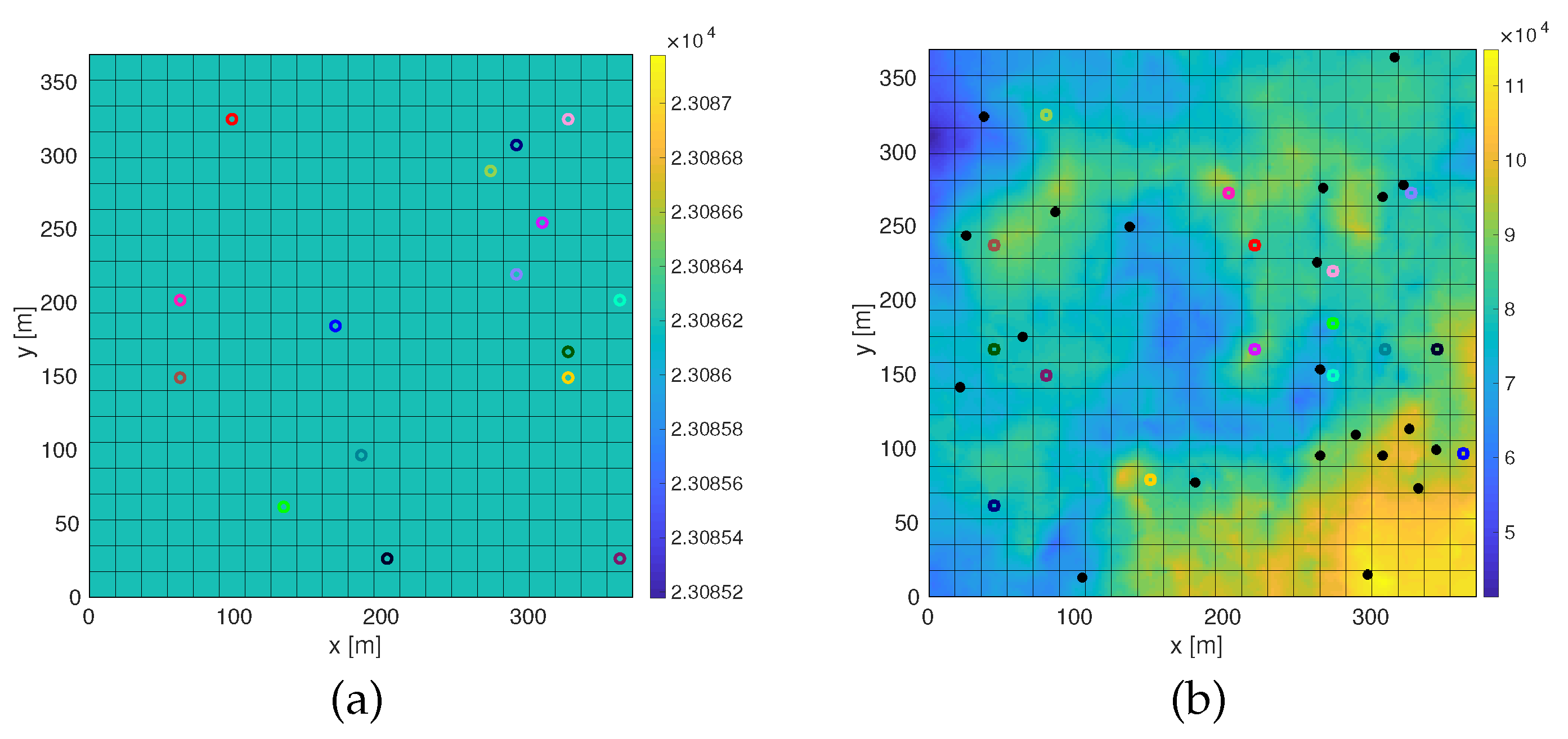
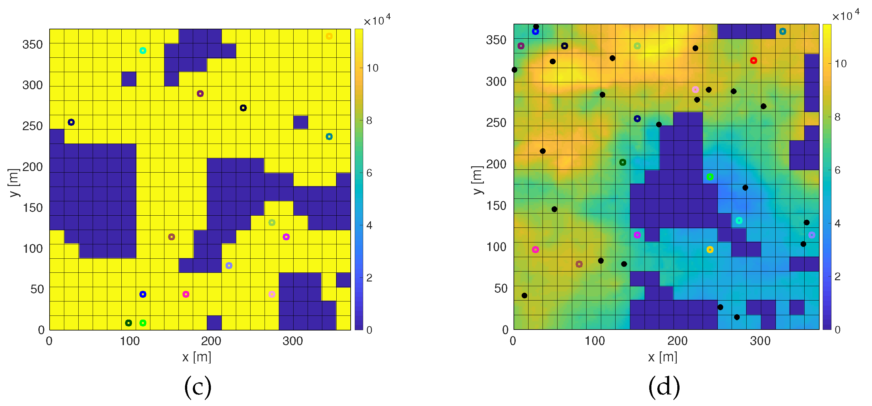
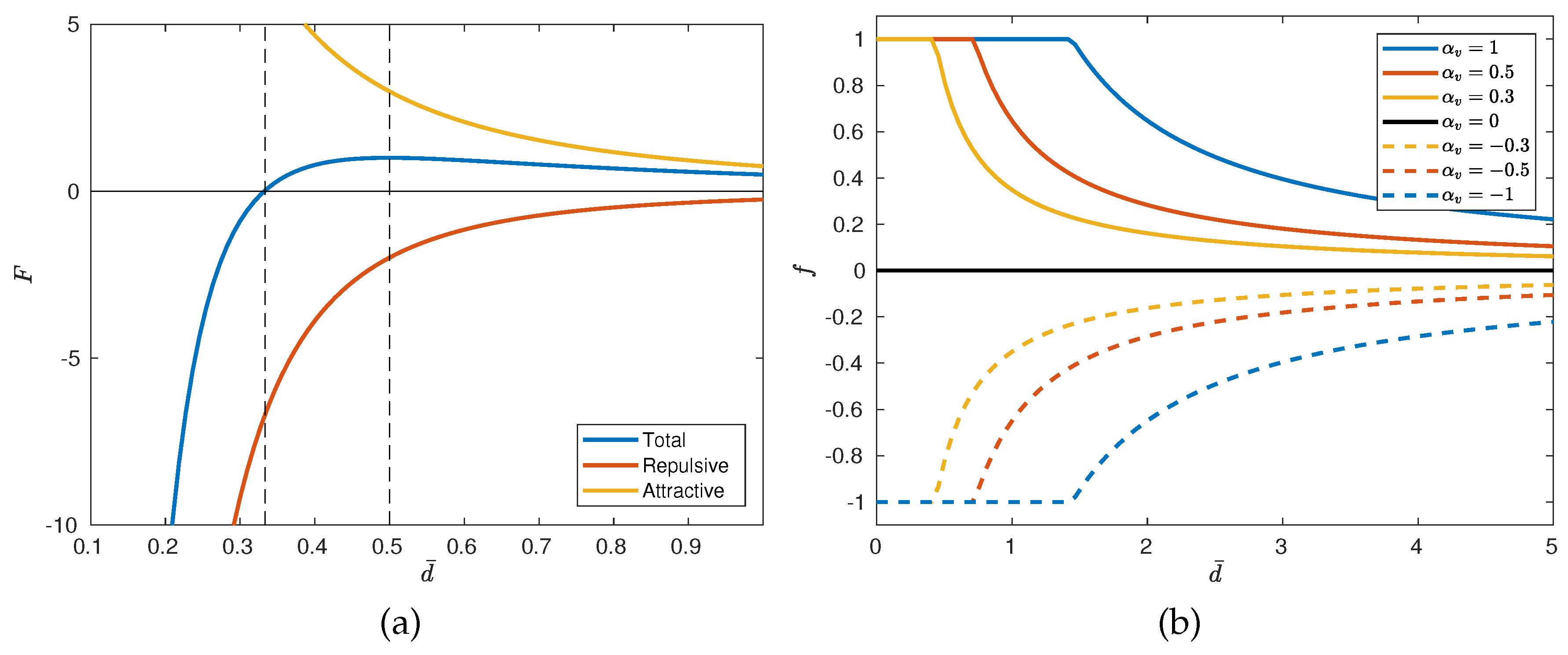
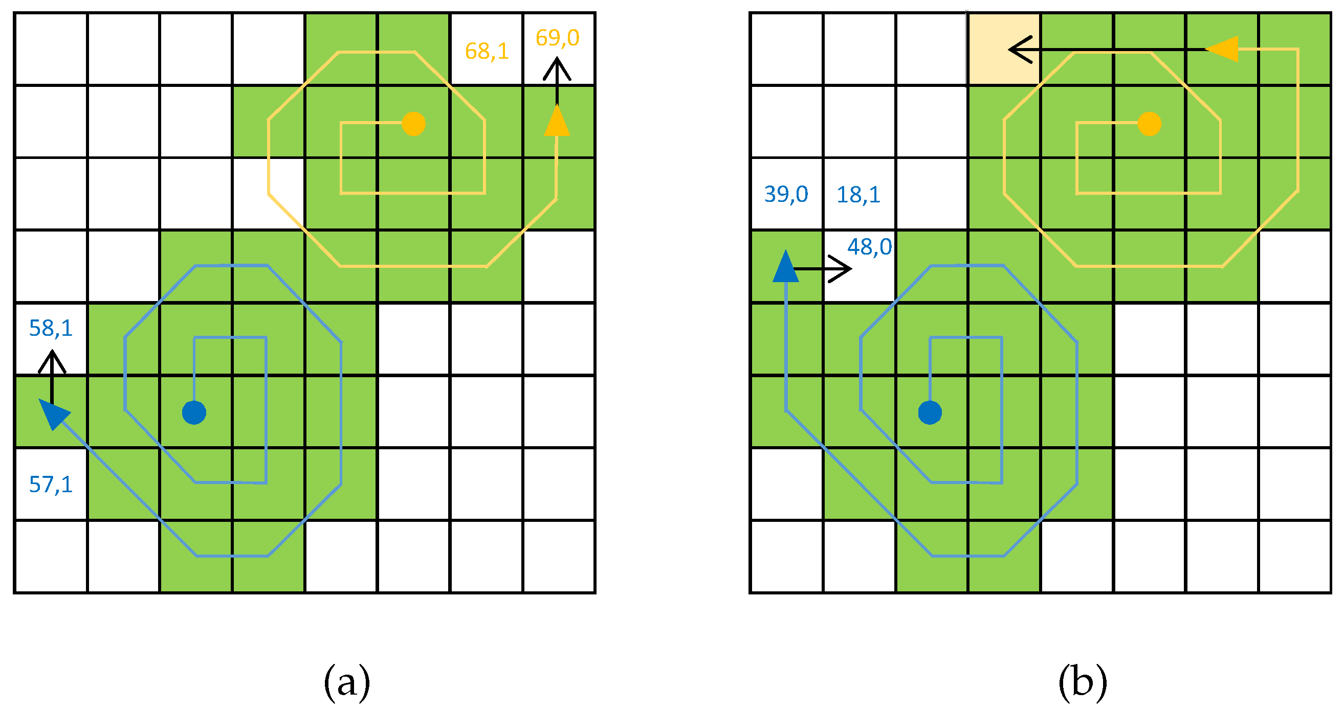
Table 1.
List of parameters that define the scenario.
| Parameter | Description | Range of Values |
|---|---|---|
| Search area per agent | [2, 15] m | |
| Number of agents | [2, 30] | |
| Nominal velocity of the agents | [2, 20] m/s | |
| Radius of the sensor footprint | [5, 20] m | |
| Aspect ratio of the search area | [0.25, 1] |
Table 2.
List of parameters that define the model of the agent.
| Parameter | Description | Equation | Value |
|---|---|---|---|
| Velocity reduction time due to | (6) | 5 s | |
| Energy-distance coefficient | (7) | 0.1 m | |
| Energy-change-of-heading coefficient | (8) | 2 | |
| Max available energy | (9) | 180 |
Table 3.
Parameters related to the search behavior for each of the three layers.
| L1 | 0 | 0 | ||||||
| L2 | 0 | 0 | 0 | |||||
| L3 | 0 | 0 | 0 | −1 |
Table 4.
Efficiencies and fitness values for each algorithm, based on the three models depicted in Section 2.4.
Table 4.
Efficiencies and fitness values for each algorithm, based on the three models depicted in Section 2.4.
| Model 1 | Model 2 | Model 3 | ||||
|---|---|---|---|---|---|---|
| Eff | Fit | Eff | Fit | Eff | Fit | |
| A1: Behaviors set | 0.70 | 0.58 | 0.57 | 0.49 | 0.39 | 0.29 |
| A2: Random | 0.61 | 0.21 | 0.57 | 0.20 | 0.09 | 0.03 |
| A3: Closest | 0.75 | 0.68 | 0.62 | 0.57 | 0.36 | 0.27 |
| A4: Boundary | 0.78 | 0.67 | 0.59 | 0.53 | 0.31 | 0.22 |
| A5: Energy | 0.66 | 0.21 | 0.59 | 0.19 | 0.16 | 0.04 |
| A6: Billiard | 0.61 | 0.23 | 0.55 | 0.22 | 0.16 | 0.05 |
| A7: Lanes | 0.73 | 0.68 | 0.61 | 0.57 | 0.35 | 0.28 |
Table 5.
Relative efficiencies and fitness values for each algorithm and each scenario type.
| Plain | Probability | Obstacles | Prob. + Obs. | |||||
|---|---|---|---|---|---|---|---|---|
| Eff | Fit | Eff | Fit | Eff | Fit | Eff | Fit | |
| A1: Behaviors set | 1 | 1 | 1 | 1 | 1 | 1 | 1 | 1 |
| A2: Random | 0.23 | 0.09 | 0.22 | 0.14 | 0.24 | 0.13 | 0.21 | 0.18 |
| A3: Closest | 0.91 | 0.93 | 0.81 | 0.86 | 0.87 | 0.84 | 0.76 | 0.77 |
| A4: Boundary | 0.78 | 0.78 | 0.63 | 0.72 | 0.86 | 0.84 | 0.66 | 0.71 |
| A5: Energy | 0.41 | 0.15 | 0.42 | 0.28 | 0.44 | 0.20 | 0.43 | 0.34 |
| A6: Billiard | 0.42 | 0.17 | 0.43 | 0.31 | 0.45 | 0.22 | 0.44 | 0.37 |
| A7: Lanes | 0.90 | 0.99 | 0.76 | 0.90 | 0.59 | 0.60 | 0.52 | 0.53 |
© 2018 by the authors. Licensee MDPI, Basel, Switzerland. This article is an open access article distributed under the terms and conditions of the Creative Commons Attribution (CC BY) license (http://creativecommons.org/licenses/by/4.0/).
Share and Cite
MDPI and ACS Style
Garcia-Aunon, P.; Barrientos Cruz, A. Comparison of Heuristic Algorithms in Discrete Search and Surveillance Tasks Using Aerial Swarms. Appl. Sci. 2018, 8, 711. https://doi.org/10.3390/app8050711
AMA Style
Garcia-Aunon P, Barrientos Cruz A. Comparison of Heuristic Algorithms in Discrete Search and Surveillance Tasks Using Aerial Swarms. Applied Sciences. 2018; 8(5):711. https://doi.org/10.3390/app8050711
Chicago/Turabian StyleGarcia-Aunon, Pablo, and Antonio Barrientos Cruz. 2018. "Comparison of Heuristic Algorithms in Discrete Search and Surveillance Tasks Using Aerial Swarms" Applied Sciences 8, no. 5: 711. https://doi.org/10.3390/app8050711
Note that from the first issue of 2016, this journal uses article numbers instead of page numbers. See further details here.