Determination of Nonlinear Creep Parameters for Hereditary Materials


1
Kazakhstan Highway Research Institute, Almaty 050061, Kazakhstan
2
Department of Mechanics, Al-Farabi Kazakh National University, Almaty 050040, Kazakhstan
3
Department of Chemistry and Chemical Technologies, University of Calabria, 87036 Rende, Italy
*
Author to whom correspondence should be addressed.
Appl. Sci. 2018, 8(5), 760; https://doi.org/10.3390/app8050760
Submission received: 10 April 2018
/
Revised: 5 May 2018
/
Accepted: 5 May 2018
/
Published: 10 May 2018
(This article belongs to the Section Materials Science and Engineering)
Abstract
:This work proposes an effective algorithm for description of nonlinear deformation of hereditary materials based on Rabotnov’s method of isochronous creep curves. The notions have been introduced for experimental and model rheological parameters and similarity coefficients of isochronous curves. It has been shown how using them, one can find instantaneous strains at various stress levels for description of nonlinear deformation of hereditary materials at creep. Relevant equations have been determined from the nonlinear integral equation of Yu. N. Rabotnov for the application cases of Rabotnov’s fractional exponential kernel and Abel’s kernel for nonlinear deformation of hereditary materials at creep. The improved methods have been given for determination of creep parameters α, ε0, δ, β, and λ. By processing and using test results for material Nylon 6 and glass-reinforced plastic TC 8/3-250, the process has been shown for sequential implementation of the developed methods for description of linear and nonlinear deformation of these materials at creep. From the results of the experimental investigation performed by the authors of this paper, it has been determined that fine-grained, dense asphalt concrete at the temperature of 20 ± 2 °C and stresses up to 0.183 MPa at direct tension is deformed considerably in a nonlinear way. It has been shown in an illustrative way by construction of isochronous creep curves at various load durations and curves of experimental rheological parameter at various stresses. Nonlinear deformation of asphalt concrete at creep is adequately described by the proposed methods.
1. Introduction
Many natural (soils, rocks, wood, natural asphalt) and artificial (metals, their alloys, polymers, concretes, composites) materials, depending on temperature and load level, to one extent or another show their viscoelastic properties. Currently there are sufficiently developed viscoelastic theory and methods [1,2,3,4,5,6] which allow the determination and description of viscoelastic properties of the materials. One can distinguish linear and nonlinear viscoelasticity [4,5,6,7] in viscoelastic theory, as well as in elastic theory [8,9]. One can say that currently the theory and methods of linear viscoelasticity have been developed sufficiently. In spite of the fact that as far back as 1913 V. Volterra [10] proposed to describe nonlinear viscoelasticity by binary integral equation, to date, nonlinear viscoelasticity theory and methods are on the stage of development and currently calculations for strength, stability, and longevity in many branches of engineering activity are made without consideration or with poor consideration of viscoelastic properties for the materials and elements of structures.
One simple but efficient means for consideration of deformation nonlinearity for hereditary materials was proposed in 1948 by Yu. N. Rabotnov [11]. It was based on the similarity of isochronous creep curves of the materials. Meanwhile, the process of creep strain is described by the equation of Boltzmann-Volterra for linear viscoelastic materials, but strain in the left part of the equation has been replaced by the so-called “curve of instantaneous deformation”, which is determined experimentally. Yu. N. Rabotnov, as the author of the method, considers that the curve of instantaneous strain is a kind of ideal imaginary curve, which is impossible to obtain in reality, as in real conditions the strain rate is always a finite value [12,13]. It can be obtained from isochronous creep curves at finite values of time, considering them similar.
It is known that the selection of kernel of the integral equation and determination of its parameters is one of the most responsible actions in the description of mechanical behavior of viscoelastic materials. As it has been said in our previous work [14], the most universal is creep kernel in the form of the fractional exponential function of Yu. N. Rabotnov [4,5,6,11]. The fractional exponential function is well studied and a special table [15] has been developed for simplification of calculations.
Some methods for determining the parameters of Rabotnov’s fractional exponential kernel are known: direct approximation [16,17,18,19,20], the use of Laplace-Carson’s transformation [16,17,18,21,22], interpolating by Lagrange polynomial [23], and the use of Mittag-Leffler’s function [16,24].
This work proposes an effective algorithm for description of nonlinear deformation of hereditary materials based on Rabotnov’s method of isochronous creep curves, and also the methods have been improved for determination of creep kernel parameters, developed in our previous work [14].
2. Method of Isochronous Creep Curves of Yu. N. Rabotnov
2.1. Short Description of Method
An important matter in the analysis of mechanical behavior of any material is the clarification of its deformation character: linearity or nonlinearity, which is usually determined by construction of strain dependence on stress according to the results of experimental tests. A more efficient and illustrative method is known for determination of deformation nonlinearity degree for materials, proposed by Yu. N. Rabotnov [4,5,6,11]. In accordance with this method, the so-called isochronous creep curves are constructed according to the test results of samples for the materials for creep at some constant stresses.
Figure 1 represents creep curves for a material at various constant stresses. Let us draw several, for example, four vertical lines, corresponding to time moments t1, t2, t3, and t4. Each vertical line crosses four creep curves corresponding to stresses σ1, σ2, σ3, and σ4. Drawing horizontal lines from specified cross points, one can find four strain values ε1(t1), ε2(t1), ε3(t1), and ε4(t1) on the vertical axis, corresponding to time t1. According to known four values of stress and four values of strain, one can construct an isochronous creep curve corresponding to time moment t1. Making similar actions, one can construct isochronous creep curves for the material at different load durations (Figure 2). Isochronous curves allow the visual evaluation of the character (linearity or nonlinearity) and nonlinearity degree of deformation for material. It is often in practice that isochronous curves are similar. The similarity property provides an opportunity to obtain all other isochronous creep curves of a material, if one of them is known.
2.2. Nonlinear Equation and Creep Kernel
Considering the similarity property of isochronous creep curves, Yu. N. Rabotnov proposed the following nonlinear integral equation to describe the process of nonlinear deformation of hereditary materials [4,5,6,11].
where is strain at time moment t;
is stress at time moment t;
is stress at time moment τ;
is creep kernel;
t is observation time;
τ is time preceding observation time t.
Expression in the left part of integral Equation (1) represents by itself the so-called “instantaneous deformation curve”, determination of which will be given below.
Creep kernel is described by Rabotnov’s fractional exponential function [4,5,6]:
where is Rabotnov’s fractional exponential function;
λ, α, β are creep kernel parameters (λ > 0, 0 < α < 1, β > 0);
Γ(·) is gamma-function.
Inserting the expression for creep kernel (2) into integral Equation (1), and considering σ = const at creep, we obtain:
3. Methods of Determination of Linear Creep Parameters for Hereditary Materials
Nearly always one can accept that the relationship between stress and strain in materials is a linear one at weak stresses. Therefore, one can use the creep curve of a material at weak stress and apply the linear viscoelasticity approach [14] for determination of creep parameters.
3.1. Parameters α, ε0, and δ
As it is known, creep curves of materials, depending on stress level and temperature, can have two or three characteristic strain sites [26,27,28]: site I with unstabilized creep, site II with stabilized creep, and site III of accelerating creep.
Then the method is proposed, according to which it will be sufficient to consider only site I of creep curve for determination of creep parameters of a material α, ε0, and δ. Having accepted n = 0, from Equation (3) we will find:
One can see that the right part of the obtained equation contains a well-known Abel’s function with unknown parameters α and δ.
Having divided both parts of the Equation (4) into instantaneous elasticity modulus E0 for the case of linear deformed material, we will obtain:
where is conditionally instantaneous strain.
Equation (5) contains three unknown parameters ε0, α, and δ. As it has been said above, the right part contains a known Abel’s function with parameter of singularity α, which has the value within the interval (0, 1). Then parameter α will be considered as known, and unknown parameters ε0 and δ will be determined with the use of the least squares method. According to the least squares method, the values of parameters ε0 and δ should meet the following condition:
where is the sum of squares of deviations;
are values of creep strain determined experimentally;
m is number of creep strain.
From the following two partial derivatives and we find expressions for determination of the parameters ε0 and δ:
Selecting sequentially the values for parameter α from interval (0, 1) with specific step, we find the values for parameter from Equation (7). Inserting the obtained values for parameter ε0 and corresponding values for parameter of singularity α into expression (8), we determine the values for parameter .
Then inserting sequentially the obtained values for parameters α, ε0, and δ into Equation (5), we calculate the values for creep strain
Calculating under the formula
the deviations of the calculated values for creep strain from those obtained experimentally, one can select optimum values for parameters α, ε0, and δ, providing the least value of Δεi.
3.2. Parameters β and λ
Having divided both parts of Equation (3) into instantaneous elasticity modulus E0, for the case of linear strain of material, we obtain:
Let us rewrite Equation (10) in the following form, inserting notation :
Using the least squares method, we write the extremum condition, similar to condition of (6):
The following expressions are obtained for determination of parameters β and λ from two equations, composed on expressions and :
The value of parameter β is determined from Equation (14). If the equation has an unambiguous solution, then it will be the target value for parameter β > 0. It is obvious that during determination of values for parameters β and λ from Equations (14) and (15), the previously calculated values are used for parameters α and ε0.
As it is known, one of the factors which limited the wide use of creep kernel with Rabotnov’s fractional exponential function has been the fact that it was not an easy way to determine its parameters [22]. A special table has been developed [15], and with its use, the fractional exponential function has been calculated under the argument x = β t(1−α) at x ≤ 4. At x > 4 it is recommended to use asymptotic formulas of B. D. Anin [29]. Calculations have shown that the infinite series in the right part of Equation (10) are poorly converged at small values of argument x < 4.
Introduction of special notation and consideration in series (12) and (16) of not time ti, but relative time (ti/tk) have essentially increased the convergence of calculations and allowed the quick obtaining of more accurate values of the fractional exponential function practically at any values of argument.
4. Algorithm for Description of Nonlinear Deformation of Hereditary Materials
This section of the paper proposes a new method for description of nonlinear deformation of hereditary materials. This method is realized in several steps and performed in the following sequence:
a. A new parameter is introduced called the experimental rheological parameter:
where is the value of creep strain at time moment t, determined experimentally;
is instantaneous strain at time moment t = 0, determined experimentally.
Experimental rheological parameter represents by itself a normalized time function in relation to experimental instantaneous strain. It has the value equal to 1 at t = 0 and more than 1 at time values of t > 0. It shows in how many times the experimental values of creep strain are more at different time values compared with instantaneous strain, which has been also obtained experimentally.
b. The values have been calculated for the experimental rheological parameter at different time values t and stresses σ. The graphs for at various stresses σ are constructed according to the calculation results. All curves at various stresses coincide (for example, as in the work [30]) for physically linear material, i.e., we have only one mean curve for all stresses (Figure 3a). There are separate curves for various stresses (Figure 3b) for physically nonlinear material. Coincidence for some of them is not excluded.
As it has been said above, the construction of isochronous creep curves is an illustrative way for the evaluation of physical nonlinearity (linearity) of the material. Therefore, we have two ways of visual evaluation for nonlinearity (linearity) of deformation for materials: first—through experimental rheological parameter ; second—by construction of isochronous creep curves.
c. Using Rabotnov’s fractional exponential function (3) and Abel’s function (4), we approximate the experimental values of creep strain for material, obtained at minimum stress σ1. Meanwhile, we find corresponding values of creep parameters α, ε0, δ, β, and λ according to the abovementioned methods.
d. In case of creep, i.e., at σ = const from integral Equation (1) we obtain:
The right part of this integral equation is denoted through km(t):
and it is named as model (theoretical or calculation) rheological parameter.
As it is seen from Equation (19), model rheological parameter depends only on time t. Similar to experimental rheological parameter , the model rheological parameter has the value equal to 1 at t = 0 and more than 1 at t > 0. It shows in how many times the calculated values of creep strain are bigger compared with the instantaneous strain, determined by calculations. Whereas the experimental rheological parameter can be determined for all stresses, the model rheological parameter is determined only for minimum stress σ1.
e. According to Yu. N. Rabotnov’s isochronous creep curves method, we find the calculated values of instantaneous strains at various stresses under the following formula:
where is the experimental value of creep for material at fixed time ts at stress σ;
is the value of model rheological parameter at fixed time ts (similarity coefficient of isochronous creep curves according to Yu. N. Rabotnov).
f. We calculate theoretical values of creep strain at various stresses under the formula:
where is the calculated value of instantaneous strain at stress σ, obtained under the formula (20).
g. We compare calculated and experimental values of creep strain at various stresses σ.
If the comparison has shown unsatisfactory accuracy, we determine again the values of instantaneous strains at various stresses under the following formula:
where is a mean value of instantaneous strain at stress σ, obtained at some fixed times ts;
N is total number of fixed times ts.
Then the calculated values of creep strain at various stresses are made under the formula:
5. Application of Proposed Algorithm and Methods
5.1. Material Nylon 6
The works [5,20] contain test results of material Nylon 6 at stresses 5, 10, and 15 MPa. The duration of the experiment was 100 h for all stresses. Values of creep strain for material Nylon 6 at specified stresses, obtained by processing of experimental results, are represented in Table 1.
It has been also determined from the data of mentioned works that the instantaneous deformation curve of material Nylon 6 has been satisfactorily approximated by power function:
Approximation of creep strain values at minimum stress (σ = 5 MPa) using Rabotnov’s fractional exponential kernel gave the following values of creep parameters: α = 0.85, ε0 = 0.1682, β = 0.18, and λ = 1.6682.
Then the creep curve of material Nylon 6 at stress σ = 5 MPa will be described by equation
From Equation (24) at σ = 5 MPa we find that = 0.1682%. Considering this fact, we determine the model rheological parameter:
Now, one can calculate the value of creep strain at stresses 10 and 15 MPa under the formula (21). For these stresses, the values of instantaneous strain, obtained under formula (24), are equal to 0.4238% and 0.7277%, respectively.
Experimental and calculated values of creep strain for material Nylon 6 at all three stresses are shown in Figure 4. As it is seen, convergence of calculated strains to experimental ones is good.
5.2. Glass-Reinforced Plastic TC 8/3-250
Samples of glass-reinforced plastic TC 8/3-250 have been tested for creep at the temperature of 23.5 ± 2 °C in the works [21,31]. As the glass-reinforced plastic is an anisotropic material, the samples have been cut along textile warp (Ѳ = 90°) and at an angle of Ѳ = 45° to them.
5.2.1. Ѳ = 90°
Values of creep strain for glass-reinforced plastic (Ѳ = 90°) at four stresses are represented in Table 2.
Test results have shown that the sample of glass-reinforced plastic, cut at an angle of Ѳ = 90° to textile warp, is deformed linearly at a specific temperature and up to stress 349 MPa. Instantaneous strain has been satisfactorily approximated by equation:
Creep strains at minimum stress, equal to 104.7 MPa, have been approximated by Rabotnov’s fractional exponential kernel. Creep parameters have the following values: α = 0.8, ε0 = 0.3501, β = 0.3, and λ = 0.0462.
The equation of creep curve for glass-reinforced plastic (Ѳ = 90°) at minimum stress (σ = 104.7 MPa) has the form of:
From Equation (27) at σ = 104.7 MPa we obtain: = 0.3501%. Considering this, we determine the model rheological parameter:
We calculate the values of instantaneous strain under Equation (27) at stresses 209.4 MPa, 279.2 MPa, and 349.0 MPa: = 0.6982%, 0.9309%, and 1.1636%, respectively.
Now using the obtained values of instantaneous strain , under formula (21) we can calculate the values of creep strain at stresses 209.4 MPa, 279.2 MPa, and 349.0 MPa.
The experimental and calculated values of creep strain for glass-reinforced plastic (Ѳ = 90°) at all four stresses are shown in Figure 5 for comparison. As it is seen, convergence of calculated creep strains to experimental ones is good.
5.2.2. Ѳ = 45°
Values of creep strain for glass-reinforced plastic (Ѳ = 45°) at six stresses are represented in Table 3.
According to test results, it has been determined that the samples of glass-reinforced plastic, cut at the angle of Ѳ = 45° to textile warp, have been deformed nonlinearly at the tested temperature and applied stresses.
Creep strains at minimum stress, equal to 20.3 MPa, have been approximated by Rabotnov’s fractional exponential kernel. The following values have been obtained for creep parameter: α= 0.8, ε0 = 0.1093, β = 0.32, and λ = 0.2459.
Considering the obtained values of parameters α, ε0, β, and λ, the equation of creep curve for glass-reinforced plastic (Ѳ = 45°) at minimum stress (σ = 20.3 MPa) has a form of:
Processing of test results allowed determination of the following values of instantaneous strain for stresses 20.3 MPa, 40.6 MPa, 60.9 MPa, 81.2 MPa, 101.5 MPa, and 121.8 MPa: 0.1093%, 0.1982%, 0.5911%, 1.3872%, 2.4874%, and 3.9975%, respectively.
The model rheological parameter has a form of:
Using the abovementioned values of instantaneous strain, one can calculate values of creep strain at all other stresses under formula (21).
Figure 6 shows experimental and calculated values of creep strain for glass-reinforced plastic (Ѳ = 45°) at all considered stresses. It is seen that convergence of experimental strains to the calculated ones is good.
5.3. Asphalt Concrete
Hot dense asphalt concrete of type B which meets the requirements of the Kazakhstan standard ST RK 1225-2013 [32] was prepared with use of aggregate fractions of 5–10 mm (20%), 10–15 mm (13%), 15–20 mm (10%) from Novo-Alekseevsk rock pit (Almaty region), sand of fraction 0–5 mm (50%) from the plant “Asphaltconcrete-1” (Almaty city), and activated mineral powder (7%) from Kordai rock pit (Zhambyl region).The used crushed stone meets the requirements of the standard of Kazakhstan ST RK 1284-2004 [33].
In this paper, bitumen of grade 100–130 has been used which meets the requirements of the Kazakhstan standard ST RK 1373-2013 [34].The bitumen grade on Superpave is PG 64-40 [35]. Bitumen has been produced by Pavlodar processing plant from crude oil of Western Siberia (Russia) by the direct oxidation method. Bitumen content of grade 100–130 in the asphalt concrete is 4.8% by weight of dry mineral material.
Samples of the hot asphalt concrete in the form of a rectangular prism with the length of 150 mm, width of 50 mm, and height of 50 mm were manufactured in the following way. Firstly, the asphalt concrete samples were prepared in the form of a square slab by means of the Cooper compactor (UK, model CRT-RC2S) according to the standard EN 12697-33 [36]. Then the samples were cut from the asphalt concrete slabs in the form of a prism. Deviations in sizes of the beams didn’t exceed 2 mm.
Tests of the asphalt concrete samples on creep at the temperature of 22 ± 2 °C were carried out according to the direct tensile scheme in specially contracted equipment. The detailed information regarding characteristics of bitumen, asphalt concrete, and equipment can be found in the work [28].
The stresses were constant during the tests and equal to 0.041, 0.074, 0.111, 0.148, and 0.183 MPa. Durations for tests have been accepted as similar ones and equal to 570 s. 10 parallel asphalt concrete samples have been tested at each constant stress.
Mean values of creep strain for the tested 10 asphalt concrete samples are represented in Table 4.
Creep curves of asphalt concrete at various stresses, constructed according to data of Table 4, are represented in Figure 7. As it is seen, the creep curves represent by themselves the lines which change monotonously with the increase of stress duration. The value of instantaneous strain (at t = 0) and slope of creep curves increase with the increase of stress.
Then, using the values of stresses and strains, which correspond to various load durations, one can construct the isochronous creep curves (Figure 8). As it is seen, the asphalt concrete is deformed considerably in a nonlinear way at the given temperature, and the nonlinearity degree of relationship between stress and strain has been increased with the stress and strain duration increase. Nonlinearity of strain for asphalt concrete has been noted by other researchers [37,38]. It should be also noted that the isochronous creep curves are similar ones. The property of similarity gives an opportunity to obtain all other isochronous creep curves, if any of them is known.
At present, it has been accepted in road science and practice that mechanical properties of asphalt concrete depend on the value and duration of the applied load and temperature, and this dependence can be described in a sufficiently accurate way with the use of linear viscoelasticity theory [39,40,41,42]. The essential nonlinearity of asphalt concrete strain determined above shows the unacceptability of linear viscoelasticity theory and necessitates the use of nonlinear viscoelasticity theory.
Graphs of experimental rheological parameter at various stresses, constructed according to the calculation results under formula (17) with the use of data of Table 4, are shown in Figure 9.
It is clearly seen that experimental rheological parameters of the asphalt concrete at various stresses do not merge into one curve; most of them diverge considerably from each other, which also shows the essential nonlinearity of the asphalt concrete strain at the considered temperatures and stresses.
Creep curves of the asphalt concrete at minimum stress, equal in our case to 0.041 MPa, have been approximated by Equation (5) with the use of Abel’s kernel and the following values have been obtained for creep parameters: α = 0.3, ε0 = 0.058, δ = 0.0138. Experimental and calculated creep curves of the asphalt concrete at the stress are represented in Figure 10 for comparison, which shows clearly that experimental creep curve of the asphalt concrete has been satisfactorily approximated by the equation of linear viscoelasticity with the use of Abel’s kernel.
Then the values of instantaneous strain are required to calculate under formula (20) at other stresses. For this purpose, we select one value of load duration, for example, 570 s. Under the following expression, we obtain the value of calculated rheological parameter:
According to the expression (32), we find that km (570) = 2.6745 for the selected load duration and at known values of creep parameters α and δ. We have values of creep strain, equal to 0.1759%, 0.2349%, 0.3632%, and 0.5741%, respectively from Table 4 at t = 570 for stresses 0.074 MPa, 0.111 MPa, 0.148 MPa, and 0.183 MPa. According to formula (20) we find the following values of instantaneous strain of the asphalt concrete equal to 0.0658%, 0.0878%, 0.1358%, and 0.2147% at the abovementioned stresses.
Now the calculated values of creep strain for the asphalt concrete at various stresses, except for minimum ones, can be determined under formula (21). It is found out that calculated values of creep strain in initial time moments at maximum stress equal to 0.183 MPa do not sufficiently converge with experimental ones. Therefore, we redetermine the value of instantaneous strain at this stress under formula (22), having included into the calculation the values of experimental creep strain and model rheological parameter at t = 90,150, 270, and 570 s. The new value of instantaneous strain at stress 0.183 MPa has been obtained, which is equal to 0.2037.
Calculated and experimental creep curves of the asphalt concrete at all stresses in comparison are represented in Figure 11. As it is seen, the calculated curves converge with sufficient accuracy with experimental ones at all stresses.
6. Conclusions
- Using the schematic creep curves and isochronous curves, Yu. N. Rabotnov’s isochronous creep curve method has been visually explained. The nonlinear integral equation has been shown for mathematical description of the nonlinear deformation process for hereditary materials, proposed by Yu. N. Rabotnov.
- Relevant equations have been determined from the nonlinear integral equation of Yu. N. Rabotnov for the application cases of Rabotnov’s fractional exponential kernel and Abel’s kernel for nonlinear deformation of hereditary materials at creep. The improved methods have been given for determination of creep parameters α, ε0, δ, β, and λ.
- The detailed method has been developed for description of the nonlinear deformation process for hereditary materials. The notions have been introduced for experimental and model rheological parameters and similarity coefficients of isochronous curves. It has been shown how using them, one can find instantaneous strains at various stress levels for description of nonlinear deformation of hereditary materials at creep.
- By processing and using test results for material Nylon 6 and glass-reinforced plastic TС 8/3-250, the process has been shown for sequential implementation of the developed methods for description of linear and nonlinear deformation of these materials at creep. The accuracy of the proposed methods is high.
- By the results of experimental investigation, performed by the authors of this paper, it has been determined that fine-grained dense asphalt concrete at the temperature of 20 ± 2 °С and stresses up to 0.183 MPa at direct tension is deformed considerably in a nonlinear way. It has been shown in an illustrative way by construction of isochronous creep curves at various load durations and curves of experimental rheological parameter at various stresses. Nonlinear deformation of the asphalt concrete at creep is adequately described by the proposed methods.
Author Contributions
Alibai Iskakbayev and Bagdat Teltayev conceived and designed the experiments; Alibai Iskakbayev, Bagdat Teltayev, Cesare Rossi and Gulzat Yensebayeva performed the experiments; Alibai Iskakbayev, Bagdat Teltayev, Cesare Oliviero Rossi and Gulzat Yensebayeva analysed the data; Alibai Iskakbayev, Bagdat Teltayev, Cesare Oliviero Rossi and Gulzat Yensebayeva contributed reagents/materials/analysis tools; Alibai Iskakbayev, Bagdat Teltayev, Cesare Oliviero Rossi and Gulzat Yensebayeva wrote the paper.
Conflicts of Interest
The authors declare no conflict of interest.
References
- Cristensen, R. Theory of Viscoelasticity: An Introduction; Academic Press: New York, NY, USA, 1971. [Google Scholar]
- Tschoegl, N. The Phenomenological Theory of Linear Viscoelastic Behavior: An Introduction; Springer: Berlin/Heidelberg, Germany, 1989. [Google Scholar]
- Ferry, J. Viscoelastic Properties of Polymers, 3rd ed.; Willey: New York, NY, USA, 1980. [Google Scholar]
- Rabotnov, Y. Mechanics of Deformed Solid Body; Nauka: Moscow, Russia, 1988. [Google Scholar]
- Rabotnov, Y. Creep of Structure Elements; Nauka: Moscow, Russia, 1966. [Google Scholar]
- Rabotnov, Y. Elements of Hereditary Mechanics of Solids; Nauka: Moscow, Russia, 1977. [Google Scholar]
- Georgievskiy, D.V.; Klimov, D.M.; Pobedrya, B.E. Peculiarities for behavior of viscoelastic materials. Solid Mech. 2004, 1, 119–157. [Google Scholar]
- Timoshenko, S.; Goodier, J. Theory of Elasticity; McGraw-Hill: New York, NY, USA, 1970. [Google Scholar]
- Lurie, A.I. Theory of Elasticity; Springer: Berlin/Heidelberg, Germany, 2005. [Google Scholar]
- Volterra, V. LeconsSurles Fonctions de Lignes; Gautheir-Villard: Paris, France, 1913. [Google Scholar]
- Rabotnov, Y.N. Balance of the elastic medium with an aftereffect. Appl. Math. Mech. 1948, 12, 53–62. [Google Scholar]
- Rabotnov, Y.; Mileiko, S. Short-Term Creep; Nauka: Moscow, Russia, 1970. [Google Scholar]
- Rabotnov, Y. Introduction to Fracture Mechanics; Nauka: Moscow, Russia, 1987. [Google Scholar]
- Iskakbayev, A.; Teltayev, B.; Alexandrov, S. Determining the creep parameters of linear viscoelastic materials. J. Appl. Math. 2016, 2016, 6568347. [Google Scholar] [CrossRef]
- Rabotnov, Y.; Papernik, L.; Zvonov, E. Tables of a Fractional Exponential Function of Negative Parameter and Its Integral; Nauka: Moscow, Russia, 1969. [Google Scholar]
- Golub, V.P.; Fernati, P.V.; Lyashenko, Y.G. Determining the parameters of the fractional exponential heredity kernels of linear viscoelastic materials. Int. Appl. Mech. 2008, 44, 963–974. [Google Scholar] [CrossRef]
- Zvonov, E.N.; Malinin, N.I.; Papernik, L.K.; Tseitlin, B.M. Determination of the creep characteristics of linear elastic hereditary materials by using a digital computer. Mech. Solid 1968, 5, 76–82. [Google Scholar]
- Gavrilov, D.А.; Markov, B.A. Numerical method of determining the rheologic parameters of composites from test results. Mech. Compos. Mater. 1987, 22, 417–421. [Google Scholar] [CrossRef]
- Mosin, A.V. Calculation of parameters for nonlinear determining equation of hereditary type. Probl. Mech. Eng. Reliab. Mach. 2002, 2, 83–88. [Google Scholar]
- Suvorova, Y.V.; Alekseyeva, S.I. Engineering applications of nonlinear-hereditary model considering the temperature. Industrial laboratory. Diagn. Mater. 2000, 66, 48–52. [Google Scholar]
- Suvorova, Y.V.; Mosin, A.V. Determination of parameters of the Rabotnov’s fractional exponential function with use of integral transform and modern software. Probl. Mech. Eng. Autom. 2002, 4, 54–56. [Google Scholar]
- Suvorova, Y.V.; About, Y.N. Rabotnov’s nonlinear hereditary equation and its applications. News Russ. Acad. Sci. Mech. Solids 2004, 1, 174–181. [Google Scholar]
- Osokin, A.E.; Suvorova, Y.V. Nonlinear governing equation of hereditary media and methods for determination of its parameters. Appl. Math. Mech. 1978, 42, 1108–1114. [Google Scholar]
- Rozovskii, M.I. Some features of elasticity hereditary media. News USSR Acad. Sci. 1961, 2, 30–36. [Google Scholar]
- Lodge, A.S. Elastic Liquids: An Introductory Vector Treatment of Finite-Strain Polymer Rheology; Academic Press: London, UK; New York, NY, USA, 1964. [Google Scholar]
- Iskakbayev, A.I.; Teltayev, B.B.; Andriadi, F.K.; Estayev, K.Z.; Suppes, E.A.; Iskakbayeva, A.A. Experimental research of creep, recovery and fracture processes of asphalt concrete under tension. In Proceedings of the 24th International Congress on Theoretical and Applied Mechanics, Montreal, QC, Canada, 21–26 August 2016. [Google Scholar]
- Iskakbayev, A.I.; Teltayev, B.B.; Rossi, C.O. Deformation and strength of asphalt concrete under static and step loadings. In Proceedings of the AIIT International Congress on Transport Infrastructure and Systems (TIS 2017), Rome, Italy, 10–12 April 2017; pp. 3–8. [Google Scholar]
- Iskakbayev, A.I.; Teltayev, B.B.; Rossi, C.O. Steady-state creep of asphalt concrete. Appl. Sci. 2017, 7, 142. [Google Scholar] [CrossRef]
- Annin, B.D. Asymptotic expansion of an exponential function of fractional order. Appl. Math. Mech. 1961, 25, 796–798. [Google Scholar] [CrossRef]
- Maksimov, R.D.; Jirgens, L.; Jansons, J.; Plume, E. Mechanical properties of polyester polymer-concrete. Mech. Compos. Mater. 1999, 35, 99–110. [Google Scholar] [CrossRef]
- Rabotnov, Y.N.; Papernik, L.H.; Stepanychev, E.I. Nonlinear creep of glass-reinforced plastic TС8/3-250. Mech. Polym. 1971, 3, 391–397. [Google Scholar]
- ST RK 1225-2013. Hot Mix Asphalt for Roads and Airfields; Technical Specifications: Astana, Kazakhstan, 2013. [Google Scholar]
- ST RK 1284-2004. Crushed Stone and Gravel of Dense Rock for Construction Works; Technical Specifications: Astana, Kazakhstan, 2004. [Google Scholar]
- ST RK 1373-2013. Bitumens and Bitumen Binders. Oil Road Viscous Bitumens; Technical Specifications: Astana, Kazakhstan, 2013. [Google Scholar]
- Asphalt Institute. Performance Graded Asphalt Binder Specification and Testing; Superpave Series No. 1; Asphalt Institute: Lexington, MA, USA, 2003. [Google Scholar]
- EN 12697-33. Bituminous Mixtures. Test Methods for Hot Mix Asphalt. Part 33: Specimen Prepared by Roller Compactor; European Committee for Standardization: Brussels, Belgium, 2003. [Google Scholar]
- Fitzgerald, J.E.; Vakili, J. Non linear characterization of sand-asphalt concrete by means of permanent-memory norms. Exp. Mech. 1973, 13, 504–510. [Google Scholar] [CrossRef]
- Basalov, Y.G.; Kuznetsov, V.N.; Shesterikov, S.A. Determination of ratio for rheonom material. Mech. Solid Body 2000, 6, 69–89. [Google Scholar]
- Yoder, E.J.; Witczak, M.W. Principles of Pavement Design; John Wiley & Sons Inc.: Hoboken, NJ, USA, 1975; p. 736. [Google Scholar]
- Huang, Y.H. Pavement Analysis and Design, 2nd ed.; Pearson Education, Inc.: Upper Saddle River, NJ, USA, 2004. [Google Scholar]
- MS-4. The Asphalt Handbook, 7th ed.; Asphalt Institute: Lexington, MA, USA, 2008. [Google Scholar]
- Papagiannakis, A.; Masad, E. Pavement Design and Materials; John Wiley & Sons, Inc.: Hoboken, NJ, USA, 2008. [Google Scholar]
Figure 1.
Creep curves of a material at various constant stresses.

Figure 2.
Isochronous deformation curves of a material.

Figure 3.
Curves of experimental rheological parameter Ke(t) at various stresses σ: (a) for physically linear material; (b) for physically nonlinear material.
Figure 3.
Curves of experimental rheological parameter Ke(t) at various stresses σ: (a) for physically linear material; (b) for physically nonlinear material.
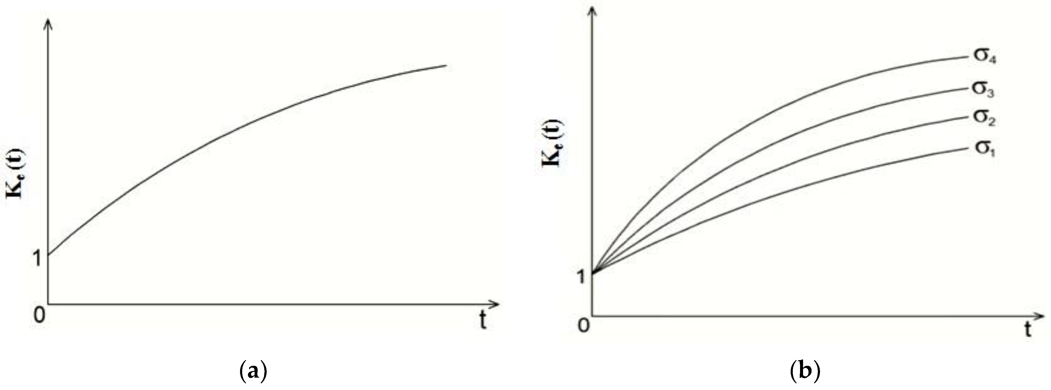
Figure 4.
Creep curves of material Nylon 6 at various stresses: 1–5 MPa; 2–10 MPa; 3–15 MPa.
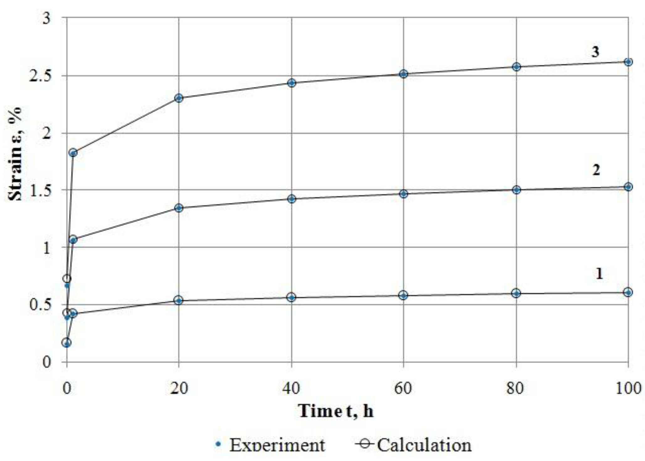
Figure 5.
Creep curves of glass-reinforced plastic (Ѳ = 90°) at various stresses: 1–104.7 MPa, 2–209.4 MPa, 3–279.2 MPa, 4–349.0 MPa.
Figure 5.
Creep curves of glass-reinforced plastic (Ѳ = 90°) at various stresses: 1–104.7 MPa, 2–209.4 MPa, 3–279.2 MPa, 4–349.0 MPa.

Figure 6.
Creep curves of glass-reinforced plastic (Ѳ = 45°) at various stresses: 1–20.3 MPa, 2–40.6 MPa, 3–60.9 MPa, 4–81.2 MPa, 5–101.5 MPa, 6–121.8 MPa.
Figure 6.
Creep curves of glass-reinforced plastic (Ѳ = 45°) at various stresses: 1–20.3 MPa, 2–40.6 MPa, 3–60.9 MPa, 4–81.2 MPa, 5–101.5 MPa, 6–121.8 MPa.
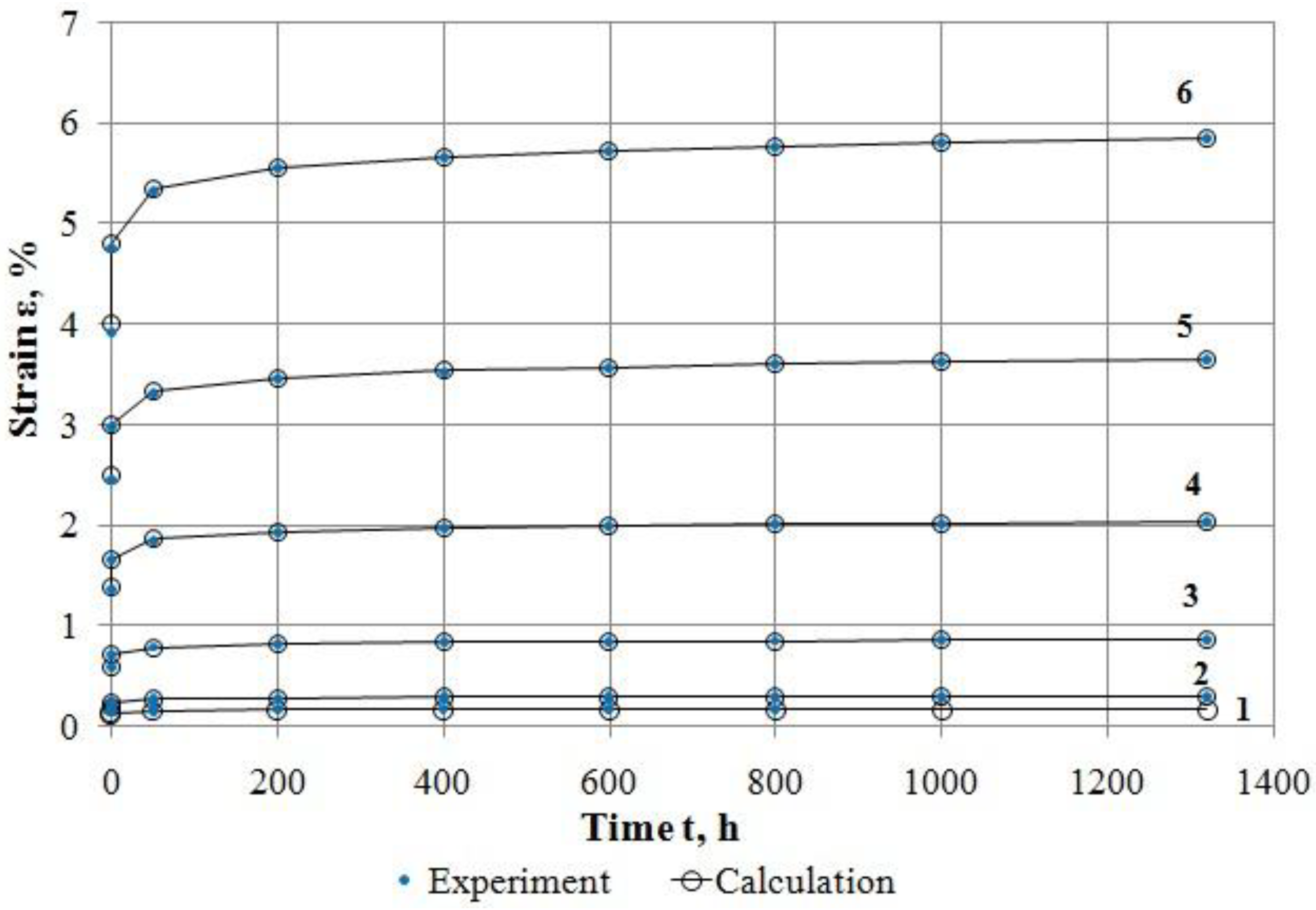
Figure 7.
Creep curves of the asphalt concrete at various stresses.

Figure 8.
Isochronous creep curves of the asphalt concrete.

Figure 9.
Graphs of experimental rheological parameter of the asphalt concrete at various stresses.

Figure 10.
Experimental and calculated creep curves of the asphalt concrete at stress 0.041 MPa.

Figure 11.
Experimental and calculated creep curves of the asphalt concrete at various stresses.


Table 1.
Creep strain values of material Nylon 6.
| Time t, h | Strain εе (t), %, at Stress σ, MPa | ||
|---|---|---|---|
| 5 | 10 | 15 | |
| 0 | 0.1537 | 0.3873 | 0.6650 |
| 1 | 0.4200 | 1.0585 | 1.8174 |
| 20 | 0.5321 | 1.3408 | 2.3022 |
| 40 | 0.5621 | 1.4164 | 2.4319 |
| 60 | 0.5804 | 1.4624 | 2.5110 |
| 80 | 0.5937 | 1.4961 | 2.5689 |
| 100 | 0.6043 | 1.5229 | 2.6148 |
Table 2.
Values of creep strain for glass-reinforced plastic (Ѳ = 90°).
| Time t, h | Strain εе (t), %, at Stress σ, MPa | |||
|---|---|---|---|---|
| 104.7 | 209.4 | 279.2 | 349.0 | |
| 0 | 0.3478 | 0.6957 | 0.9276 | 1.1595 |
| 1 | 0.3616 | 0.7232 | 0.9643 | 1.2054 |
| 10 | 0.3668 | 0.7337 | 0.9782 | 1.2228 |
| 50 | 0.3709 | 0.7419 | 0.9892 | 1.2365 |
| 100 | 0.3728 | 0.7457 | 0.9942 | 1.2428 |
| 200 | 0.3746 | 0.7493 | 0.9991 | 1.2489 |
| 300 | 0.3757 | 0.7515 | 1.0020 | 1.2525 |
| 400 | 0.3765 | 0.7530 | 1.0040 | 1.2550 |
| 500 | 0.3771 | 0.7542 | 1.0056 | 1.2570 |
Table 3.
Values of creep strain for glass-reinforced plastic (Ѳ = 45°).
| Time t, h | Strain εе (t), %, at Stress σ, MPa | |||||
|---|---|---|---|---|---|---|
| 20.3 | 40.6 | 60.9 | 81.2 | 101.5 | 121.8 | |
| 0 | 0.1074 | 0.1946 | 0.5805 | 1.3624 | 2.4430 | 3.9262 |
| 1 | 0.1302 | 0.2359 | 0.7037 | 1.6515 | 2.9614 | 4.7593 |
| 50 | 0.1457 | 0.2639 | 0.7873 | 1.8478 | 3.3134 | 5.3251 |
| 200 | 0.1518 | 0.2750 | 0.8204 | 1.9255 | 3.4527 | 5.5489 |
| 400 | 0.1548 | 0.2806 | 0.8370 | 1.9643 | 3.5222 | 5.6608 |
| 600 | 0.1566 | 0.2838 | 0.8466 | 1.9869 | 3.5629 | 5.7260 |
| 800 | 0.1579 | 0.2861 | 0.8533 | 2.0027 | 3.5912 | 5.7715 |
| 1000 | 0.1588 | 0.2878 | 0.8586 | 2.0150 | 3.6132 | 5.8068 |
| 1320 | 0.1600 | 0.2900 | 0.8649 | 2.0300 | 3.6401 | 5.8500 |
Table 4.
Values of creep strain for asphalt concrete.
| Time t, h | Strain εе (t), %, at Stress σ, MPa | ||||
|---|---|---|---|---|---|
| 0.041 | 0.074 | 0.111 | 0.148 | 0.183 | |
| 0 | 0.0475 | 0.0543 | 0.0805 | 0.1313 | 0.1782 |
| 30 | 0.0633 | 0.0728 | 0.1018 | 0.1584 | 0.2305 |
| 90 | 0.0849 | 0.0932 | 0.1338 | 0.1782 | 0.2855 |
| 150 | 0.0988 | 0.1102 | 0.1491 | 0.2084 | 0.3310 |
| 210 | 0.1099 | 0.1232 | 0.1643 | 0.2484 | 0.3710 |
| 270 | 0.1194 | 0.1346 | 0.1795 | 0.2696 | 0.4081 |
| 330 | 0.1255 | 0.1457 | 0.1937 | 0.2839 | 0.4482 |
| 390 | 0.1339 | 0.1546 | 0.2055 | 0.3184 | 0.4812 |
| 450 | 0.1415 | 0.1627 | 0.2158 | 0.3293 | 0.5105 |
| 510 | 0.1460 | 0.1713 | 0.2273 | 0.3478 | 0.5433 |
| 570 | 0.1488 | 0.1759 | 0.2349 | 0.3632 | 0.5741 |
© 2018 by the authors. Licensee MDPI, Basel, Switzerland. This article is an open access article distributed under the terms and conditions of the Creative Commons Attribution (CC BY) license (http://creativecommons.org/licenses/by/4.0/).
Share and Cite
MDPI and ACS Style
Iskakbayev, A.; Teltayev, B.; Oliviero Rossi, C.; Yensebayeva, G. Determination of Nonlinear Creep Parameters for Hereditary Materials. Appl. Sci. 2018, 8, 760. https://doi.org/10.3390/app8050760
AMA Style
Iskakbayev A, Teltayev B, Oliviero Rossi C, Yensebayeva G. Determination of Nonlinear Creep Parameters for Hereditary Materials. Applied Sciences. 2018; 8(5):760. https://doi.org/10.3390/app8050760
Chicago/Turabian StyleIskakbayev, Alibai, Bagdat Teltayev, Cesare Oliviero Rossi, and Gulzat Yensebayeva. 2018. "Determination of Nonlinear Creep Parameters for Hereditary Materials" Applied Sciences 8, no. 5: 760. https://doi.org/10.3390/app8050760
Note that from the first issue of 2016, this journal uses article numbers instead of page numbers. See further details here.