Automatic Selection of Low-Permeability Sandstone Acoustic Emission Feature Parameters and Its Application in Moisture Identification

Featured Application

This study proposed an automatic AE feature parameters selection method. The potential application is the preprocessing of AE signal before low-permeability sandstone moisture identification.

Abstract

Moisture is a vital factor in the structural stability of sandstone, which is the main component of low-permeability reservoir rocks. Hence, studies into moisture identification are crucial. Diverse information about rock, such as its structural and mechanical parameters, can be obtained from the acoustic emission (AE) signal. However, the types of AE parameters are varied, and the rock information that is represented by them is different. Traditional methods of parameter selection are mostly based on the correlation between parameters and the experience of researchers, which are not accurate when the correlation between parameters is fuzzy and does not meet automation requirements. In this study, a method of signal feature selection based on a data fluctuation rule and clustering analysis is proposed. This method takes the fluctuation law of the signal itself and the correlation degree of cluster labels as the basis, and the selection step is divided into two steps. An experimental platform is established, and uniaxial compression on sandstones with different moisture contents is carried out to verify the efficiency of this method. The selected feature parameters are used for moisture classification combined with a support vector machine (SVM) classifier, and the identification results verify the efficiency of energy security monitoring in low-permeability rocks.

1. Introduction

Sandstone has connected pores and good hydrophilicity. Moisture can affect the pore distribution and permeability of sandstone, in turn influencing the storage and percolation capacity of the reservoir [1]. The distribution and production of energy resources, such as oil and natural gas, will change consequently. Moreover, structural stability is crucial in resource mining engineering with high stress and osmotic pressure, such as in petroleum exploitation and natural gas excavation. Moisture can change the mechanical properties of rock, and then promote the growth of rock cracks under loading. Collapse accidents may happen due to unqualified rock moisture content. Therefore, moisture identification in low-permeability reservoir rocks is of significance. The stress distribution is uneven under loading because of the differences in the crystal microstructure and the inhomogeneous distribution of pores in rock mass [2,3]. Acoustic emission (AE) occurs when a high-energy state produced in a stress concentration region releases energy in the form of a transient elastic wave to achieve a steady state [4,5]. The excitation mode of AE is diverse. Besides the solid medium, AE can also be generated through liquid medium, and its application in detection engineering is extensive. For example, AE can be generated by cavitation phenomena and turbulent flows associated with fluid leaks [6]. Indeed, even if some drawbacks with respect to other methods may be identified, AE analysis has been successfully adopted for leak detection in pipelines [7,8]. In the field of rock engineering, AE stems from the particle slip and crack propagation in rock, and the frequency bands are mostly between 20–200 K, which are imperceptible to humans [9]. The signal feature parameters can be extracted through signal acquisition and processing technology; thus, the relation between the signal and rock damage state can be analyzed, and this method is called parametric analysis [10,11,12,13]. This method has been used successfully by many scholars to conduct structural health monitoring. Static tensile loading was conducted on aluminum plates in aerospace systems by Z. Kral et al., and the identification of the damaged part was realized with a combination of artificial neural networks [14]. H.Y. Sim et al. [15] realized the valve abnormalities detected in a reciprocating compressor by means of AE technology and wave packet transform. B.A. Zarate et al. [16] completed estimations of the damage location in liquid-filled tanks with the methods of AE technology and probabilistic algorithms. R. Gutkin et al. conducted various test configurations on carbon fiber-reinforced plastics including tension, compression, and compact tension (CT) to collect the AE data [17]; the signals were analyzed by a machine learning method, and the frequency domain rule of this material in damage was obtained.

There are dozens of kinds of feature parameters in a sandstone AE signal, and each parameter can reflect some aspects of the signal characteristics [18]. On the one hand, the types of parameter that are needed are diverse due to the difference of reservoir material under research. On the other hand, the change rules of parameters are various because of differences in the geological environment, or there are no quantifiable change rules. Too many feature parameters not only hinder classification, but also complicate the exploration of mineral resources and monitoring of reservoir structures. Thus, it is important to conduct a reasonable selection of parameters and minimize redundancy while also ensuring differences among parameter types. Scholars from different countries have achieved several positive results in signal feature selection. For example, Gowid et al. [19] proposed a fault AE signal feature selection method based on a Fast Fourier Transform (FFT) for high-speed centrifugal equipment and verified the feasibility by experiments. T Warren carried out grinding operations [20] to get the AE signal, and then used autoregressive modeling and discrete wavelet decomposition for feature extraction. The optimal features were obtained by three different feature selection methods, and the superiority of the extraction and selection method was proved through comparative experiments.

There are many kinds of traditional feature selection and dimensionality reduction methods, such as Principal Component Analysis (PCA), the Pearce coefficient method, etc. [21,22,23,24]. Most of these methods carry out feature fusion and reconstruction, or abandon certain features according to the correlation between features [25,26]. These methods are feasible when the feature dimension is large enough; however, the evaluation of the correlation between features is difficult to carry out, and the accuracy of those methods will decrease when the feature dimension is less, or correlation between the features is fuzzy. In this study, the AE signal of sandstone is taken as the research object in combination with the petrophysical characteristics of low-permeability reservoirs. Here, we propose a method for feature selection by using the fluctuation law of single feature parameters and clustering analysis. This method doesn’t need to use the correlation between features. The research emphasis is on the analysis of the parameters’ own fluctuation law and the correlation between cluster labels and original labels. The reservoir rocks are porous, and the AE signal feature has fewer dimensions (usually less than 100). The uncertainty of correlation between features is higher in comparison with other types of signal; thus, the two-step method is especially suitable for feature selection in low-permeability reservoir rock, and then, the energy security in the process of underground exploration can be improved.

The remainder of this paper is organized as follows. The flow of the two-step algorithm is shown in Section 2. In the first step, the operation of standardized, mean, and tolerance calculations are completed in turn. In the second step, the algorithm-switching rule is proposed according to the silhouette value criterion. Then, the label correlations are calculated, and the AE parameters are selected through the quantitative relationship of the threshold. Section 3 presents the parameter selection experiment. The experimental system and samples are described. Six parameters are extracted from the AE signal, and the two-step method is used to conduct parameter selection. Section 4 concerns moisture identification and algorithm comparison. The moisture identification results of two other selection algorithms are compared with the two-step method. The rationality of the two-step method in low-permeability rock moisture identification is tested. In addition, the signal variability and handling method in actual engineering applications are also stated in Section 4. Section 5 summarizes the method process, clarifies the application scenario and proposes the future work plan.

2. Method

Assume vector $X=(X_1,X_2\dots X_i\dots X_n)$ is the $n$ characteristic of the AE signal, and the vector $Y=(Y_1,Y_2\dots Y_j\dots Y_m)$ is the $m$ labels of the signal, where $i\in [1,n],j\in [1,m]$. The number of each feature is $k$ and one feature is expressed as follows:

$${\mathit{X}}_{\mathit{i}}=\left[\begin{array}{cccc}{a}_1^{(1)}& a_2^{(1)}& \dots & a_m^{(1)}\\ a_1^{(2)}& a_2^{(2)}& \dots & a_m^{(2)}\\ \dots & \dots & \dots & \dots \\ a_1^{(k)}& a_2^{(k)}& \dots & a_m^{(k)}\end{array}\right]$$

(1)

where each line represents a feature sample with a known label, and each column represents a label. The overall flow of the algorithm is shown in Figure 1.

2.1. First Step Selection

(1) Standardized operation

The purpose of standardized operation is to eliminate the influence of the different dimensions on the threshold setting. Assume that the maximum and minimum values in the feature vector $X_i$ are $a_j^{(q)}{|}_{max}$ and $a_j^{(q)}{|}_{min}$, where $h_{max}$ and $h_{min}$ are the maximum and minimum values of the normalized interval, respectively. The elements in $X_i$ are standardized by Equation (1).

$$a_j^{(q)}{|}_{nor}=h_{min}+(a_j^{(q)}-a_j^{(q)}{|}_{min})*\frac{h_{max}-h_{min}}{a_j^{(q)}{|}_{max}-a_j^{(q)}{|}_{min}},$$

(2)

where $q\in [1,k],j\in [1,m]$ and the normalized feature matrix is expressed as follows:

$$X_i{|}_{nor}=\left[\begin{array}{cccc}{a}_1^{(1)}{|}_{nor}& a_2^{(1)}{|}_{nor}& \dots & a_m^{(1)}{|}_{nor}\\ a_1^{(2)}{|}_{nor}& a_2^{(2)}{|}_{nor}& \dots & a_m^{(2)}{|}_{nor}\\ \dots & \dots & \dots & \dots \\ a_1^{(k)}{|}_{nor}& a_2^{(k)}{|}_{nor}& \dots & a_m^{(k)}{|}_{nor}\end{array}\right]$$

(3)

(2) Mean operation

Suppose the feature vectors after mean operation is $X_i^{\prime }{|}_{nor}$, then:

$$X{\prime }_i{|}_{nor}=(a_1,a_2\dots a_m)=(\frac{1}{k}{\displaystyle \sum _{q=1}^k{a}_1^{(q)}{|}_{nor}},\frac{1}{k}{\displaystyle \sum _{q=1}^k{a}_2^{(q)}{|}_{nor}}\dots \frac{1}{k}{\displaystyle \sum _{q=1}^k{a}_m^{(q)}{|}_{nor}})$$

(4)

(3) Tolerance calculation operation

Calculate and obtain the tolerance vector between groups $P=(p_1,p_2\dots p_{m-1})$, where $p_1=|a_2-a_1|,p_2=|a_3-a_2|,\dots ,p_{m-1}=|a_m-a_{m-1}|$. Prescribe the threshold as $p_{thre}$; then, count the number of elements less than $p_{thre}$ in the vector $P$, which is denoted as $r$. Then, prescribe the threshold as $r_{thre}$, and judge the size relationship between $r$ and $r_{thre}$. Retain this feature if $r$ is less than $r_{thre}$, and discard this feature if $r_{thre}$ is less than $r$. The theoretical range of p_thre is (0, +∞), and the value is related to the h_max and h_min in standardized operation. The theoretical range of $r_{thre}$ is [0, m − 1]. With the difference of research area, the fluctuation of parameters is diverse. Hence, the idea of machine learning is referred to during the definitions of $p_{thre}$ and $r_{thre}$. The initial thresholds can be determined manually. Then, the moisture identification model, whose input vector is the feature parameters selected by the two-step method, can be trained using mass data. The thresholds can be adjusted to obtain the optimal effect.

2.2. Second Step Selection

Assume that $X\prime =(X_{1,}{X}_2,\dots X_v)$ is the feature vector retained in the first step; this is usually $v\le n$, because the original number of features is $n$. Assume that $X_i$ is a feature vector in $X\prime$ and the corresponding matrix of real features and labels $G$ is expressed as follows:

$$G=\left[\begin{array}{cccc}(a_1^{(1)}{|}_{nor},Y_{1,1})& (a_2^{(1)}{|}_{nor},Y_{1,2})& \dots & (a_m^{(1)}{|}_{nor},Y_{1,m})\\ (a_1^{(2)}{|}_{nor},Y_{2,1})& (a_2^{(2)}{|}_{nor},Y_{2,2})& \dots & (a_m^{(2)}{|}_{nor},Y_{2,m})\\ \dots & \dots & \dots & \dots \\ (a_1^{(k)}{|}_{nor},Y_{k,1})& (a_2^{(k)}{|}_{nor},Y_{k,2})& \dots & (a_m^{(k)}{|}_{nor},Y_{k,m})\end{array}\right]$$

(5)

The clustering method is used to obtain cluster labels, and K-means, linkage, and gmdistribution are considered as alternatives, because the applicability of different data is different for clustering algorithms [27,28]. K-means determines the optimal class by iteratively calculating the distance between the sample and the centroid. Linkage calculates the similarity of different data, and sorts them to obtain a category. Gmdistribution converges to a local optimum with iterative computation. The silhouette value criterion is taken to obtain the best clustering algorithm and algorithms switched for different types of data.

(1) Silhouette value criterion

The silhouette value describes the state of cohesion and the degree of separation, which is an important parameter for evaluating the effect of clustering [29,30]. The range of silhouette values is between −1 and 1; the larger the value, the better the clustering result. The concrete implementation steps are as follows:

• Assume that $x_i$ is one of the elements, calculating the distance between $x_i$ and all of the other elements within its own cluster. Take the mean of the distance and denote it as $a_i$, which is used to quantify the cohesion.
• Randomly take another cluster $b_j$, and calculate the average distance between $a_i$ and all of the elements in the cluster $b_j$.
• Traverse all of the clusters and find the minimum average distance and denote it as $b_j\prime$, which is used to quantify the separation.
• The silhouette value of $x_i$ is $s_i=({b\prime }_j-a_i)/max(a_i,{b\prime }_j)$.
• Calculate the silhouette value of each element, and obtain the mean as the overall silhouette value of the current clustering.

(2) The algorithm switching rule is as follows:

• Select two features randomly in the feature vector as samples to carry an algorithm comparison; assume that the selected features are $X_u$ and $X_w$.
• The optimal number of clusters needs to be determined firstly in order to compare the fitness of the three clustering algorithms. Since the numbers of the signal labels are $m$, cluster and calculate the silhouette value using those three algorithms respectively. Then, average them when the number of clusters is $2,3\dots m$. Assume that the result is $B_{u2},B_{u3}\dots B_{um}$ for $X_u$, and the result is $B_{w2},B_{w3}\dots B_{wm}$ for $X_w$.
• Define $B_u=max\{B_{u2},B_{u3}\dots B_{um}\}$ and $B_w=max\{B_{w2},B_{w3}\dots B_{wm}\}$. Let $K_u$ equal the number of clusters corresponding to $B_u$, and let $K_w$ equal the number of clusters corresponding to $B_w$; thus, $K_u$ and $K_w$ are the optimal number of clusters for each feature.
• The selection of the optimal clustering algorithm can be started after determination of the optimum number of clusters. Take $K_u$ as the number of clusters, carry out cluster analysis out on the feature $X_u$, and assume the silhouette value is $M_{u1}$, $M_{u2}$, and $M_{u3}$ when the clustering algorithm is K-means, linkage, and gmdistribution, respectively. Take $K_w$ as the number of clusters, carry out cluster analysis on the feature $X_w$, and assume that the silhouette value is $M_{w1}$, $M_{w2}$ and $M_{w3}$ when the clustering algorithm is K-means, linkage, and gmdistribution, respectively.
• Assume:

  $$M=max\{\frac{1}{2}(M_{u1}+M_{w1}),\frac{1}{2}(M_{u2}+M_{w2}),\frac{1}{2}(M_{u3}+M_{w3})\}$$

  (6)

K-means will be chosen if $M=\frac{1}{2}(M_{u1}+M_{w1})$, linkage will be chosen if $M=\frac{1}{2}(M_{u2}+M_{w2})$, and gmdistribution will be chosen if $M=\frac{1}{2}(M_{u3}+M_{w3})$.

(3) Cluster analysis

Set the number of clusters to $m$ and cluster using the optimum algorithm obtained in the previous step. The labels of the original features correspond to the labels obtained by clustering, and the relation matrix is denoted as $G\prime$:

$$G^{\prime }=\left[\begin{array}{cccc}(a_1^{(1)}{|}_{nor},{Y^{\prime }}_{1,1})& (a_2^{(1)}{|}_{nor},{Y^{\prime }}_{1,2})& \dots & (a_m^{(1)}{|}_{nor},{Y^{\prime }}_{1,m})\\ (a_1^{(2)}{|}_{nor},{Y^{\prime }}_{2,1})& (a_2^{(2)}{|}_{nor},{Y^{\prime }}_{2,2})& \dots & (a_m^{(2)}{|}_{nor},{Y^{\prime }}_{2,m})\\ \dots & \dots & \dots & \dots \\ (a_1^{(k)}{|}_{nor},{Y^{\prime }}_{k,1})& (a_2^{(k)}{|}_{nor},{Y^{\prime }}_{k,2})& \dots & (a_m^{(k)}{|}_{nor},{Y^{\prime }}_{k,m})\end{array}\right]$$

(7)

(4) Label correlation calculation

Define $E={\displaystyle \sum _{l=1}^k{\displaystyle \sum _{d=1}^m\left|{Y^{\prime }}_{l,d}-Y_{l,d}\right|}}$ as the label correlation and $E_{thre}$ as the threshold. Discard this feature if $E\ge E_{thre}$, which means that the difference between the original distribution and the clustering label is too big. Retain this feature if $E<E_{thre}$, which means that the difference is small enough.

3. Parameter Selection Experiment

In order to verify the rationality of the two-step method, an experimental system was set up to carry out uniaxial compression tests on sandstones with different moisture contents. This section will elaborate on the experimental process, equipment, and sample state. The AE signals’ feature parameters were extracted, and the two-step method was used to realize their selection. The main objective of this section was to implement and refine the proposed two-step method.

3.1. Experimental System and Sample Description

Sandstone is a sedimentary rock with good hydrophilicity and brittleness [31,32,33]. Sandstone is one of the most important components of reservoirs; many oil and gas fields around the world are made up of it. Samples with a moisture content of 0% (drying state), 25%, 50%, 75%, and 100% (saturation state) were obtained separately by weighing. The data acquisition system comprised a pressure apparatus, a piezoelectric resonance sensor, a signal processing board, and a principal computer (Figure 2). The sample and sensor were coupled by Vaseline, and vertical uniaxial compression was exerted on each stone. The AE signal was stored in an Structured Query Language (SQL) database on the principal computer after the operations of amplification, filtering, and Analog/Digital conversion.

The dimensions of the sandstone samples were 15 cm × 15 cm × 2 cm. To ensure the consistency of the AE data, the AE sensor was installed on the bottom left corner of the sample, and the distance between the sensor center and sample vertex was 2 cm × 2 cm. The pressure apparatus was hydraulic, with a maximum output loading of 10 T. The range of loading in this experiment was 0–7 T, and the loading was exerted through a homogeneous velocity of 0.7 T/min. To avoid moisture evaporation, we shortened the time interval between moisture control and uniaxial compression to 30 min. The AE sensor was a resonant piezoelectric sensor produced by Pengxiang Technology Company in Changsha, China, and the model number was PXR03. The sensitivity was greater than 75 DB, and the response frequency range was 22–220 KHz. The acquisition system comprised a signal processing board and an A/D conversion module. The frequency range of the signal processing board was 20–250 KHz, and the magnification was 300. The A/D conversion module was 12 bits, and the sampling rate was 1 MHz.

3.2. Extraction of Feature Parameters

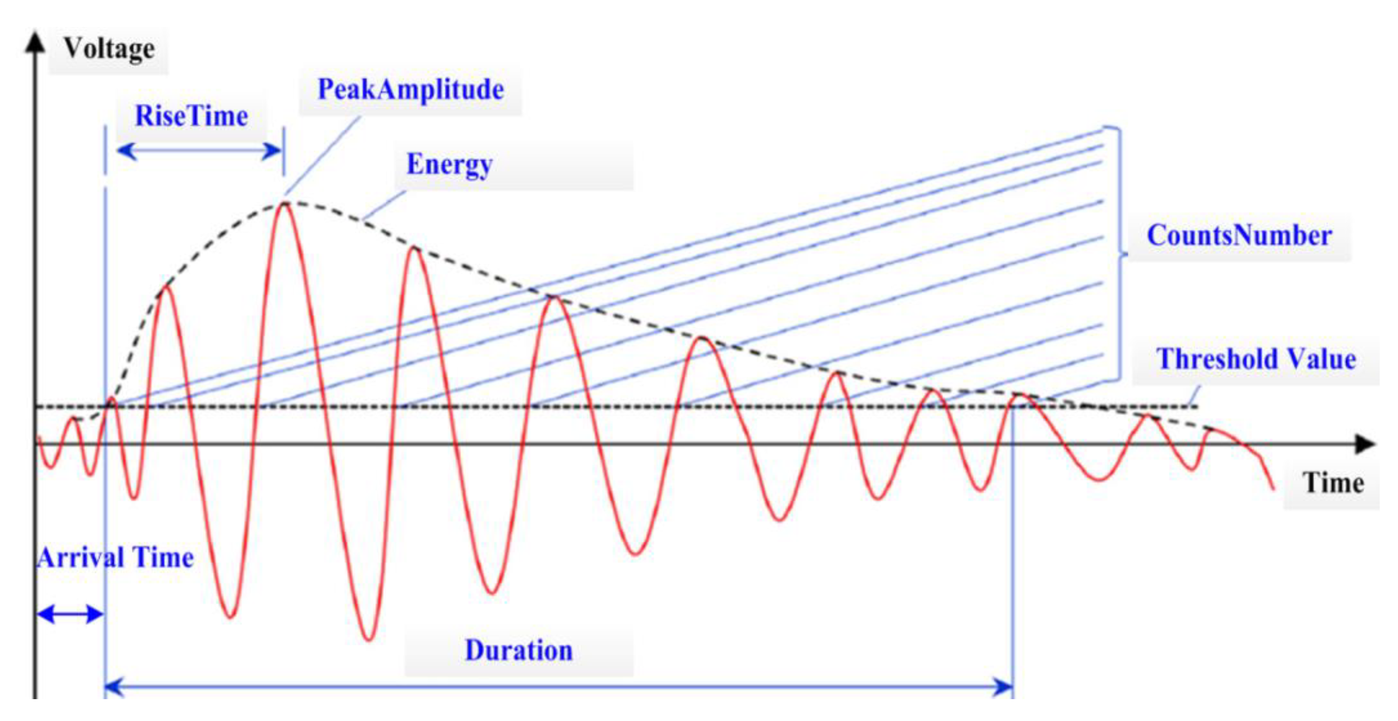
The types of traditional time-domain feature parameters in AE signals are multitudinous, among which the energy, duration, count numbers, rise time, arrival time, and peak amplitude have been widely studied (Figure 3). Thus, they are chosen to explore the variation regulation with moisture content. The definitions of each AE parameter are as follows:

• Energy: The area under the signal envelope.
• Duration: The time interval between the signal first coming over the threshold until it attenuates to the threshold.
• Count numbers: The number of times the signal comes over the threshold.
• Rise time: The time interval between the signal first coming over the threshold and reaching amplitude.
• Arrival time: The time point at which the signal first comes over the threshold.
• Peak amplitude: The maximum amplitude of the signal.

The AE wave amplitudes after the signal processing board and AD conversion module were mainly concentrated between 800–1000 mV. Wave amplitudes exceeding a defined threshold should be considered a useful signal, and the signals below the threshold should be considered noise [34]. By measurement, the amplitude of electromagnetic interference noise on the signal processing board was 160 mV approximately, and the threshold voltage was set to 180 mV. Hence, the noise can be filtered, and the AE can be validated.

There were 100 samples of each rock sample with different moisture content, which were numbered 1–100. The samples’ number was taken as abscissa, and the parameters were taken as ordinate. The feature parameters of samples with different moisture contents are shown in Figure 4.

3.3. Selection of Feature Parameters

3.3.1. First Step Selection

Firstly, the above six AE parameters are standardized to eliminate the influence of different dimensions on the threshold setting, where the $h_{max}$ is set as 100, and the $h_{min}$ is set as 0. Then, all of the values of the parameters for each sample are averaged, and the results are shown in Figure 5. Finally, the tolerance between groups is calculated, and the number of elements smaller than the tolerance threshold in the tolerance vector is obtained. Compare this number with the number threshold; the feature parameters that are greater than the number threshold are discarded. The main parameters in the first step selection are shown in

Table 1. Result of parameters in the first step.

Characteristic Parameter	${\mathit{a}}_{\mathit{j}}^{(\mathit{q})}{|}_{\mathit{m}\mathit{a}\mathit{x}}$	${\mathit{a}}_{\mathit{j}}^{(\mathit{q})}{|}_{\mathit{m}\mathit{i}\mathit{n}}$	${\mathit{a}}_1$	${\mathit{a}}_2$	${\mathit{a}}_3$	${\mathit{a}}_4$	${\mathit{a}}_5$	${\mathit{p}}_1$	${\mathit{p}}_2$	${\mathit{p}}_3$	${\mathit{p}}_4$	$\mathit{r}$
Energy	50.97 DB	40.09 DB	0.95	0.79	0.60	0.38	0.16	0.16	0.19	0.22	0.22	0
Duration	0.536 ms	0 ms	0.91	0.51	0.25	0.15	0.05	0.40	0.26	0.10	0.10	0
Counts Number	21	2	0.70	0.49	0.35	0.20	0.05	0.21	0.14	0.15	0.15	0
Rise Time	0.1683 ms	0.087 ms	0.79	0.19	0.16	0.20	0.02	0.60	0.03	0.04	0.18	2
Arrival Time	0.0901 ms	0.083 ms	0.65	0.71	0.75	0.74	0.66	0.06	0.04	0.01	0.08	4
Peak Amplitude	30.98 DB	24.70 DB	0.77	070	0.41	0.34	0.24	0.07	0.29	0.07	0.10	2

.

During the optimization of thresholds, we found that the big p_thre and the small r_thre values can lead to the incorrect deletion of effective parameters, which causes an insufficient input in moisture identification. Similarly, the small p_thre and the big r_thre can lead to the incorrect reservation of invalid parameters, which causes redundant inputs and overfitting. Neither of these cases is conducive to accurate moisture identification. In this experiment, the p_thre and r_thre values were determined to 0.09 and 3, respectively, after the iterations. Table 1 shows that the value of $r$ in Arrival Time was four, which is bigger than $r_{thre}$; thus, Arrival Time was discarded in first step selection.

3.3.2. Second Step Selection

(1) Selection of clustering algorithm

Energy and duration parameters were taken as instances to choose the optimal algorithm among K-means, linkage, and gmdistribution, using the algorithm switching rule that was mentioned above. In order to determine the optimum number of clusters, the enumeration method was used to calculate the silhouette value when the cluster was 2, 3, 4, and 5, respectively, and the results are shown in Figure 6a,b.

The average silhouette value using those three algorithms under different K values to intuitively get the optimum number of clusters was calculated, and the results are shown in Figure 6c. For the Energy parameter, the maximum silhouette value can be obtained when the K value is 5, and when the K value is 4 for the duration parameter. The silhouette value performance and main parameters used in the algorithm switching of those three clustering algorithms are shown in Figure 6d and

Table 2. Result of parameters in algorithm switching.

Feature Name	Parameter List	Parameter Value	Feature Name	Parameter List	Parameter Value	Parameter Name	Parameter Value
$X_u$	$B_{u2}$	0.565	$X_w$	$B_{w2}$	0.561	$\frac{1}{2}(M_{u1}+M_{w1})$	0.8425
	$B_{u3}$	0.857		$B_{w3}$	0.753
	$B_{u4}$	0.86		$B_{w4}$	0.525	$\frac{1}{2}(M_{u2}+M_{w2})$	0.83
	$B_{u5}$	0.857		$B_{w5}$	0.807
	$K_u$	4		$K_w$	5	$\frac{1}{2}(M_{u3}+M_{w3})$	0.48
	$M_{u1}$	0.805		$M_{w1}$	0.88
	$M_{u2}$	0.79		$M_{w2}$	0.87	$M$	0.8425
	$M_{u3}$	0.1		$M_{w3}$	0.86

, respectively (with five clusters for the Energy parameter and four clusters for the Duration parameter).

(2) Clustering analysis

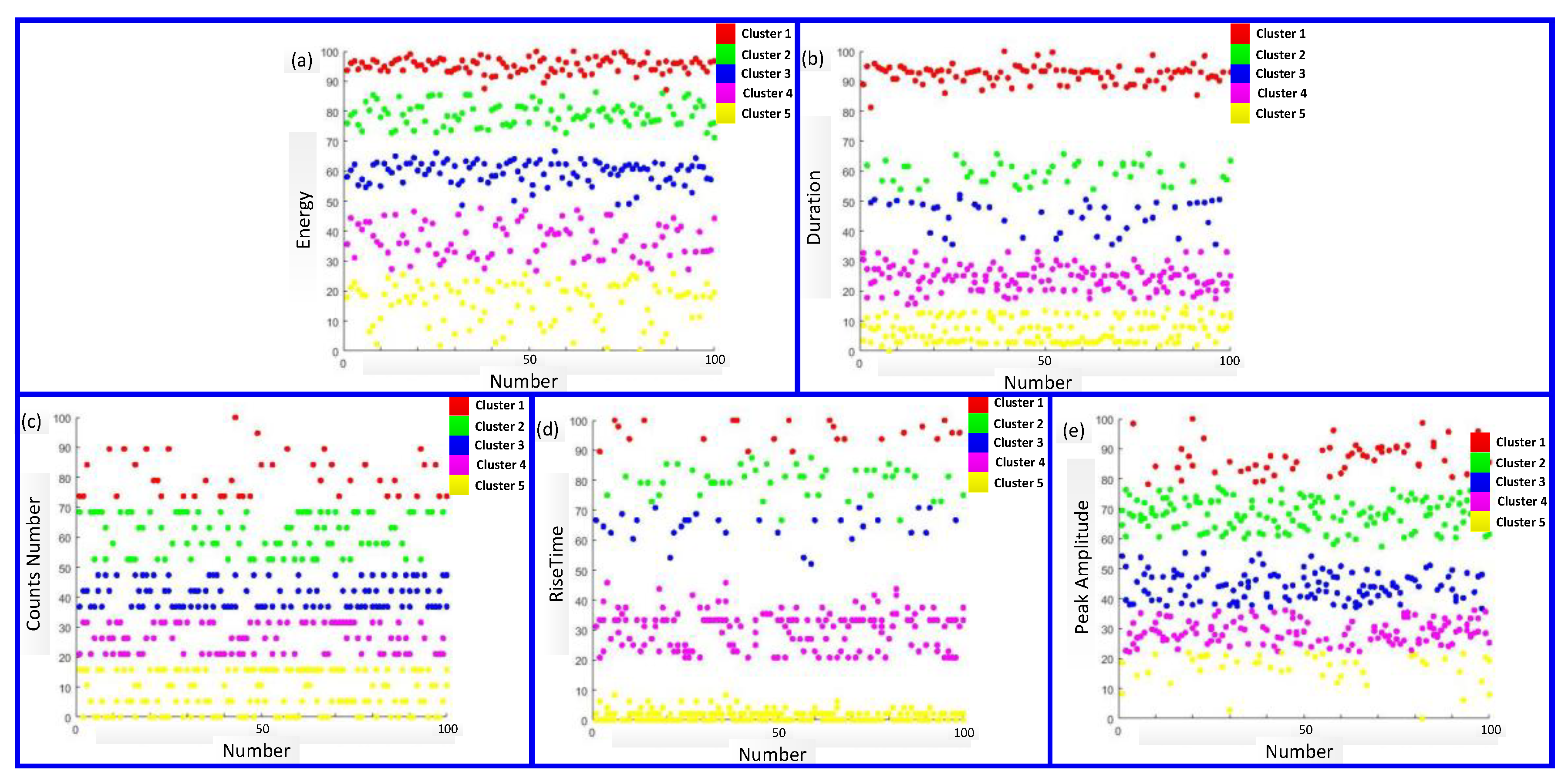
Set the number of clusters to 5 due to there being five moisture contents. The clustering results are shown in Figure 7, where the abscissa is the sample number and the ordinate is the parameter value after standardized operation.

The label correlations $E$ of the above five parameters are calculated, and the results are shown in Figure 8.

RiseTime is discarded, because its label correlation is bigger than the threshold $E_{thre}$, which is set to 300. The Arrival Time and the Rise Time were discarded among the six original parameters after two-step selection.

3.4. Experimental Analysis

The experiment shows that each step had a discarded parameter. During the first step, the fluctuation rule of the Arrival Time parameter, which can be reflected by the tolerances described in Section 2.1, was too small. Thus, the moisture content had little effect on this parameter. This parameter was redundant and should be discarded. The clustering algorithm was switched according to Equation (6). The clustering analysis was conducted to obtain label correlation, which is described at the end of Section 2.2. The clustering results were the spatial distributions of the different parameters. The label correlation of the Rise Time parameter was large, indicating that the difference between the original distribution and the clustering label was too large. Although the moisture content presented a regular change, the variation among the Rise Time parameters was mixed. The error rate can be increased if this parameter is taken as the basis for moisture identification.

4. Application of Moisture Identification and Algorithm Comparison

In order to verify the advantage of the two-step method, the AE feature parameters were selected through the two-step method. The Pearson coefficients method and and principal component analysis (PCA) were taken as input vectors for the SVM classifier to realize moisture identification. Algorithm comparisons were conducted. The AE parameter data that were used in this experiment were taken from Section 3. The experimental setup and boundary conditions, including the sandstone sample source, data acquisition equipment, and the system-computing environment, were identical to those in the experiment in Section 3.

4.1. Moisture Identification Result

Only the Energy, Duration, Counts Number, and Peak Amplitude parameters were retained after the two-step selection; thus, the four features were used to conduct the classification of rock moisture using the support vector machine (SVM) classifier. The SVM is a widely used supervised classifier that transforms non-separable samples into high-dimensional feature spaces by a non-linear mapping algorithm. There were 350 samples in the training group, with 70 samples for each moisture content. The test group consisted of 150 samples, with 30 samples for each moisture content. An identification model was obtained by training, and the identification results are shown in Figure 9a. According to the results, there were eight errors in the total of 150 test data samples, and the overall identification rate was 94.7%.

4.2. Comparison of Selection Algorithms

The Pearson coefficient method and principal component analysis method were used for the selection and dimensionality reduction of the above six feature parameters, and then compared with the two-step selection algorithm that is proposed in this study.

4.2.1. Pearson Coefficient Method

The Pearson coefficient method is used to judge the correlation between variables, and the correlation size is measured by the Pearson correlation coefficient $r$. Assume that $x$ and $y$ are variables, and the Pearson correlation coefficient can be calculated as follows:

$$r=\frac{{\displaystyle \sum _i{z}_x}{z}_y}{N-1}=\frac{{\displaystyle \sum _i(x-\overline{x})(y-\overline{y})}}{\sqrt{{\displaystyle \sum _i{(x-\overline{x})}^2}{\displaystyle \sum _i{(y-\overline{y})}^2}}},$$

(8)

where $z_x=\frac{(x-\overline{x})}{{\sigma }_x}$, $z_y=\frac{(y-\overline{y})}{{\sigma }_y}$, $\overline{x}$, $\overline{y}$ are the mean values, and ${\sigma }_x$, ${\sigma }_y$ are the standard deviations of $x$ and $y$, respectively. The value of $r$ is between −1 and 1, the two variables were linearly negative when $r$ was −1, and there was a linear positive correlation when $r$ was 1 [35]. The Pearson coefficients were calculated for the above six parameters, and the Pearson correlation coefficient matrix is shown in

Table 3. Pearson correlation coefficient matrix.

Pearson Correlation Coefficients	Energy	Duration	Counts Number	Rise Time	Arrival Time	Peak Amplitude
Energy	1.0000	0.8999	0.9129	0.6856	−0.0350	0.8657
Duration	0.8999	1.0000	0.9028	0.8140	−0.1541	0.8447
Counts Number	0.9129	0.9028	1.0000	0.7464	−0.1123	0.8152
Rise Time	0.6856	0.8140	0.7464	1.0000	−0.1400	0.6372
Arrival Time	−0.0350	−0.1541	−0.1123	−0.1400	1.0000	−0.0455
Peak Amplitude	0.8657	0.8447	0.8152	0.6372	−0.0455	1.0000

.

As shown in the Pearson correlation coefficient matrix, the Pearson correlation coefficients between Energy and Duration, Energy and Counts Number, Energy and Peak Amplitude, and Duration and Counts Number were all close to or exceeded 0.9. It can be assumed that the variables mentioned above were approximately linear, and useful information for classification will not be provided if these parameters are used at the same time. The Energy and Counts Number parameters were discarded to avoid redundancy.

4.2.2. Principal Component Analysis

Principal component analysis (PCA) is a widely used dimensionality reduction method, in which the basic idea is to transform the original data into a new coordinate system by using linear transformation and obtaining the principal components [36]. Dimensionality reduction was conducted on the six original feature parameters by PCA, and the coefficient matrix is shown in

Table 4. Coefficient matrix of principal component analysis.

Coefficient Number	1	2	3	4	5	6
1	0.0280	−0.0347	0.4634	0.0124	0.8146	−0.3458
2	0.9918	−0.1163	−0.0490	0.0161	−0.0130	−0.0039
3	0.0414	0.0057	0.8173	−0.3675	−0.4388	0.0512
4	0.1171	0.9924	0.0097	0.0104	0.0337	0.0027
5	−0.0028	−0.0059	0.3139	0.9293	−0.1943	−0.0033
6	0.0118	−0.0164	0.1272	0.0280	0.3238	0.9369

.

The components in the first four columns of the coefficient matrix were used as the projection matrix to ensure the consistency of the comparative experiment. Assume the new characteristic parameters $\overline{X}=X\times D$, where $X$ is the original sample matrix after subtracting the average value, and $D$ is the projection matrix of the first $s$ principal components, where $s$ is valued at 4.

4.2.3. Comparison of Identification Results

The feature parameters processed by the Pearson coefficient method and PCA were respectively put into the SVM classifier, keeping all the parameters constant. The identification results are shown in Figure 9b,c.

The comparative results of the three feature selection methods are shown in

Table 5. Comparison of different dimensionality reduction algorithms.

Algorithm	Two-Step Selection Method	PCA	Pearson Coefficient Method
Correct rate (%)	94.7%	91.3%	87.3%
Time overhead of feature selection (s)	20.34	14.1	13.6

. The running environments were the same, including the Win 7 professional system, Intel (R) Core (TM) i5-4590 CPU. The main frequency was 3.3 GHz, and the running memory was 8 G.

4.3. The Signal Variability and Handling Method in Actual Engineering Applications

During the AE excitation experiment, the loading was exerted homogeneously to guarantee data consistency and avoid the interference caused by collision, friction, and so on. However, the loading in a collapse process will not be produced evenly in real geotechnical engineering situations. Loading is intense, creating an abundance of abnormal data. Although statistical laws are adopted during the clustering analysis in the two-step method, the probabilities of mistaken deletion and reservation are large. The influence of abnormal interference should be considered in any actual structural monitoring engineering. In actual geotechnical engineering applications, the initial AE signal, as shown in Figure 10, is representative and least affected by load fluctuation. Hence, the initial AE signal should be captured as the source of parameter extraction to reduce abnormal data.

The floating threshold method can be used to capture the initial AE signal. Assume that the time-domain AE signal is $f(t)$, where the maximum values $f(t_1)$, $f(t_2)$···$f(t_n)$ are obtained at $t_1$, $t_2$···$t_n$. Set the capture threshold $\omega =\frac{1}{n}{\displaystyle \sum _{i=1}^{n}f(t_i)}$. The point should be determined as the waveform entrance when the $\beta$ continuous signal amplitudes are greater than the threshold; the point should be determined as the waveform exit when the $\beta$ continuous signal amplitudes are less than the threshold. The value of $\beta$ can be adjusted according to the actual needs.

4.4. Results Discussion

The overall identification rate was 94.7%, indicating that the parameters selected by the two-step method can well reflect the change effect of the moisture content. PCA maps the parameters to the new space, and the new parameter matrix can be obtained by principal component extraction. The Pearson correlation coefficient method takes the correlation between variables as its basis. The label information can be made available by the two-step method; thus, an accuracy advantage exists in rock moisture identification. Moreover, the signal variability problem in actual engineering application was also handled through the capture of the initial AE signal.

The two-step method was designed to provide more precise and differentiated input vectors for moisture identification in low-permeability sandstone. The intended usage scenario is the preprocessing of AE parameters before low-permeability sandstone moisture identification model training. The quality of sandstone AE input parameters has a great influence on the final identification result during moisture pattern identification. Redundant sandstone AE parameters will increase the computational pressure and slow down training time. Overfitting also easily occurs. On the contrary, using too few sandstone AE parameters may mean the loss of effective moisture information and lead to incorrect identification.

5. Conclusions

Moisture can not only change the macroscopic structural properties of sandstone, it also has a great influence on the storage capacity of low-permeability reservoirs. Besides, the distribution and mining safety of mineral resources, such as oil and gas, are all affected by the moisture content of reservoir rocks. Diverse AE characteristics provide an important reference for moisture identification. Hence, the rational selection of AE characteristics is of great significance to mineral resource exploration. Researchers tend to choose features based only on their subjective experience, which not only increases the workload for pattern identification in the latter stage, but also doesn’t meet the requirements of automatic monitoring. In this study, a method of feature parameter selection based on the fluctuation trend of data and clustering analysis is proposed. An experimental system is built to carry out uniaxial compression tests on sandstones with different moisture content, and six feature parameters are extracted from the original AE signals. A two-step selection method is proposed to realize the reasonable selection of feature parameters, and the identification of moisture was conducted using an SVM classifier.

Although the two-step selection method is more expensive in execution time, the advantages in the accuracy of the second classification are obvious from the identification results and the comparison of the selection algorithms. This is beneficial to energy security in low-permeability reservoir rocks. The sandstones with different moisture content were tested in the laboratory, which is an extremely controlled environment. However, there may be diverse disturbances in real geotechnical engineering situations, such as material anisotropy and environmental mechanical effects. We will conduct experiments in real environments to obtain data that is more fitting to real engineering applications in future work.

References

- Zhang, D.; Gamage, R.P.; Perera, M.; Zhang, C.; Wanniarachchi, W. Influence of Water Saturation on the Mechanical Behaviour of Low-Permeability Reservoir Rocks. Energies 2017, 10, 236. [Google Scholar] [CrossRef]
- Yin, S.; Zhang, J.; Liu, D. A study of mine water inrushes by measurements of in situ stress and rock failures. Nat. Hazards 2015, 79, 1961–1979. [Google Scholar] [CrossRef]
- Chen, G.Q.; Huang, R.Q.; Qiang, X.U.; Tian-Bin, L.I.; Zhu, M.L. Progressive Modelling of the Gravity-induced Landslide Using the Local Dynamic Strength Reduction Method. J. Mt. Sci. 2013, 10, 532–540. [Google Scholar] [CrossRef]
- Li, X. A brief review: Acoustic emission method for tool wear monitoring during turning. Int. J. Mach. Tools Manuf. 2002, 42, 157–165. [Google Scholar] [CrossRef]
- Scruby, C.B. An introduction to acoustic emission. J. Phys. E Sci. Instrum. 1987, 20, 946. [Google Scholar] [CrossRef]
- Anastasopoulos, A.; Kourousis, D.; Bollas, K. Acoustic emission leak detection of liquid filled buried pipeline. J. Acoust. Emiss. 2009, 27, 27–40. [Google Scholar]
- Martini, A.; Troncossi, M.; Rivola, A. Vibroacoustic measurements for detecting water leaks in buried small-diameter plastic pipes. J. Pipeline Syst. Eng. Pract. 2017, 8, 04017022. [Google Scholar] [CrossRef]
- Martini, A.; Troncossi, M.; Rivola, A. Leak Detection in Water-Filled Small-Diameter Polyethylene Pipes by Means of Acoustic Emission Measurements. Appl. Sci. 2016, 7, 2. [Google Scholar] [CrossRef]
- Bhuiyan, M.S.H.; Choudhury, I.A.; Dahari, M.; Nukman, Y.; Dawal, S.Z. Application of acoustic emission sensor to investigate the frequency of tool wear and plastic deformation in tool condition monitoring. Measurement 2016, 92, 208–217. [Google Scholar] [CrossRef]
- Roberts, T.M.; Talebzadeh, M. Acoustic emission monitoring of fatigue crack propagation. J. Constr. Steel Res. 2003, 59, 695–712. [Google Scholar] [CrossRef]
- Huguet, S.; Godin, N.; Gaertner, R.; Salmon, L.; Villard, D. Use of acoustic emission to identify damage modes in glass fibre reinforced polyester. Compos. Sci. Technol. 2002, 62, 1433–1444. [Google Scholar] [CrossRef]
- Elfergani, H.A.; Pullin, R.; Holford, K.M. Damage assessment of corrosion in prestressed concrete by acoustic emission. Constr. Build. Mater. 2013, 40, 925–933. [Google Scholar] [CrossRef]
- Yoon, D.J.; Jung, J.C.; Park, P.; Lee, S.S. AE characteristics for monitoring fatigue crack in steel bridge members. Proc. SPIE 2000, 3995. [Google Scholar] [CrossRef]
- Kral, Z.; Horn, W.; Steck, J. Crack propagation analysis using acoustic emission sensors for structural health monitoring systems. Sci. World J. 2013, 2013, 823603. [Google Scholar] [CrossRef] [PubMed]
- Sim, H.Y.; Ramli, R.; Saifizul, A.A.; Abdullah, M.A.K. Empirical investigation of acoustic emission signals for valve failure identification by using statistical method. Measurement 2014, 58, 165–174. [Google Scholar] [CrossRef]
- Zarate, B.A.; Pollock, A.; Momeni, S.; Ley, O. Structural health monitoring of liquid-filled tanks: A Bayesian approach for location of acoustic emission sources. Smart Mater. Struct. 2014, 24, 015017. [Google Scholar] [CrossRef]
- Gutkin, R.; Green, C.J.; Vangrattanachai, S.; Pinho, S.T.; Robinson, P.; Curtis, P.T. On acoustic emission for failure investigation in CFRP: Pattern recognition and peak frequency analyses. Mech. Syst. Signal Process. 2011, 25, 1393–1407. [Google Scholar] [CrossRef]
- Ranjith, P.G.; Jasinge, D.; Song, J.Y.; Choi, S.K. A study of the effect of displacement rate and moisture content on the mechanical properties of concrete: Use of acoustic emission. Mech. Mater. 2008, 40, 453–469. [Google Scholar] [CrossRef]
- Gowid, S.; Dixon, R.; Ghani, S. A novel robust automated FFT-based segmentation and features selection algorithm for acoustic emission condition based monitoring systems. Appl. Acoust. 2015, 88, 66–74. [Google Scholar] [CrossRef]
- Liao, T.W. Feature extraction and selection from acoustic emission signals with an application in grinding wheel condition monitoring. Eng. Appl. Artif. Intell. 2010, 23, 74–84. [Google Scholar] [CrossRef]
- Kappatos, A.V.; Dermatas, S.E. Feature Extraction for Crack Detection in Rain Conditions. J. Nondestruct. Eval. 2007, 26, 57–70. [Google Scholar] [CrossRef]
- Garrett, D.; Peterson, D.A.; Anderson, C.W.; Thaut, M.H. Comparison of linear, nonlinear, and feature selection methods for EEG signal classification. IEEE Trans. Neural Syst. Rehabil. Eng. 2003, 11, 141–144. [Google Scholar] [CrossRef] [PubMed]
- Tian, L.; Erdogmus, D.; Adami, A.; Pavel, M. Feature selection by independent component analysis and mutual information maximization in EEG signal classification. In Proceedings of the IEEE International Joint Conference on Neural Networks, Montreal, QC, Canada, 31 July–4 August 2005; pp. 3011–3016. [Google Scholar]
- Cerrada, M.; Sanchez, R.V.; Cabrera, D.; Zurita, G.; Li, C. Multi-Stage Feature Selection by Using Genetic Algorithms for Fault Diagnosis in Gearboxes Based on Vibration Signal. Sensors 2015, 15, 23903–23926. [Google Scholar] [CrossRef] [PubMed]
- Malhi, A.; Gao, R.X. PCA-based feature selection scheme for machine defect classification. IEEE Trans. Instrum. Meas. 2004, 53, 1517–1525. [Google Scholar] [CrossRef]
- Hsu, H.H.; Hsieh, C.W. Feature Selection via Correlation Coefficient Clustering. J. Softw. 2010, 5, 1371–1377. [Google Scholar] [CrossRef]
- Vermunt, J.K.; Magidson, J. Latent Class Cluster Analyses. Appl. Latent Class Anal. 2002, 11, 89–106. [Google Scholar]
- Tan, K.H.; Darus, A.B. Pattern recognition of partial discharge signal in gas insulated switchgear apparatus using visual and cluster analysis. In Proceedings of the International Conference on Power System Technology, Kunming, China, 13–17 October 2002; pp. 1842–1846. [Google Scholar]
- Campello, R.J.; Hruschka, E.R. A fuzzy extension of the silhouette width criterion for cluster analysis. Fuzzy Sets Syst. 2006, 157, 2858–2875. [Google Scholar] [CrossRef]
- Covoes, T.F.; Hruschka, E.R. Towards improving cluster-based feature selection with a simplified silhouette filter. Inf. Sci. 2011, 181, 3766–3782. [Google Scholar] [CrossRef]
- Kumar, S.; Gupta, R.C.; Shrivastava, S.; Csetenyi, L.; Thomas, B.S. Preliminary study on the use of quartz sandstone as a partial replacement of coarse aggregate in concrete based on clay content, morphology and compressive strength of combined gradation. Constr. Build. Mater. 2016, 107, 103–108. [Google Scholar] [CrossRef]
- Townend, E.; Thompson, B.D.; Benson, P.M.; Meredith, P.G.; Baud, P.; Young, R.P. Imaging compaction band propagation in Diemelstadt sandstone using acoustic emission locations. Geophys. Res. Lett. 2008, 35, 189–193. [Google Scholar] [CrossRef]
- Zorlu, K.; Gokceoglu, C.; Ocakoglu, F.; Nefeslioglu, H.A.; Acikalin, S. Prediction of uniaxial compressive strength of sandstones using petrography-based models. Eng. Geol. 2008, 96, 141–158. [Google Scholar] [CrossRef]
- Kocur, G.K.; Vogel, T. Classification of the damage condition of preloaded reinforced concrete slabs using parameter-based acoustic emission analysis. Constr. Build. Mater. 2010, 24, 2332–2338. [Google Scholar] [CrossRef]
- Logoglu, K.B.; Ates, T.K. Speeding-Up Pearson Correlation Coefficient Calculation on Graphical Processing Units. In Proceedings of the 2010 IEEE 18th Signal Processing and Communications Applications Conference, Diyarbakir, Turkey, 22–24 April 2010; pp. 840–843. [Google Scholar]
- Wold, S.; Esbensen, K.; Geladi, P. Principal component analysis. Chemom. Intell. Lab. Syst. 1987, 2, 37–52. [Google Scholar] [CrossRef]
Figure 1.
Flow chart of selection algorithm.
Figure 2.
Experimental system.
Figure 3.
Feature parameter of the acoustic emission (AE) signal.
Figure 4.
Feature parameters of samples with different moisture contents. (a)is Energy parameter; (b) is Duration parameter; (c) is Counts Number parameter; (d) is Rise Time parameter; (e) is Arrival Time parameter; (f) is Peak Amplitude parameter.
Figure 5.
Mean value of parameters with different moisture contents.
Figure 6.
(a,b) show the silhouette values using different algorithms in different clusters, where (a) is the result of the energy parameter, and (b) is the result of the duration parameter. (c) shows the mean value of silhouette value with different algorithms. (d) shows the performance of different algorithms in terms of silhouette value.
Figure 7.
Output of clustering. (a) is Energy parameter; (b) is Duration parameter; (c) is Counts Number parameter; (d) is Rise Time parameter; (e) is Peak Amplitude parameter.
Figure 8.
Label correlations of different parameters.
Figure 9.
Output of comparative experiment using the support vector machine (SVM), where (a) is the result of the two-step-method, (b) is the result of principal component analysis (PCA), and (c) is the Pearson coefficient method.
Figure 10.
The initial AE signal.