Non-Contact and Real-Time Measurement of Kolsky Bar with Temporal Speckle Interferometry

Abstract

In this paper, a new non-contact and real-time measurement system for Kolsky bars is presented. This system uses two sets of temporal speckle interferometry in-plane displacement measurement devices to replace two strain gauges of conventional Kolsky bars. The in-plane displacement measurement of the Kolsky bar is mainly intended to provide a new test method for the dynamic mechanical properties of small-size material samples with diameters below 2 mm. This method is non-contact, does not require any intermediate medium, and can make the Kolsky bar applicable to characterizing the dynamic mechanical properties of materials under higher strain rates and smaller size conditions. The measuring devices and principles are described. In addition, a preliminary experiment is carried out to demonstrate the performance of this new device.

1. Introduction

In the fields of aviation, aerospace, packaging, transportation, and other areas of military and civil engineering, the materials used will encounter stress events such as explosions, rapid collision, and other impact load. It is of great practical significance to study the dynamic mechanical properties of materials under high strain rate conditions for engineering design and application. The Kolsky bar (also known as Split Hopkinson Pressure Bar) apparatus is the most popular and convenient system for characterizing the high strain-rate behaviors of materials [1].

The typical Kolsky bar is using two strain gages that past on the incident bar and transmitter bar to measure the dynamic mechanical properties of a material under high strain rate conditions. This method requires good adhesion between the bar and the strain gauge. Apart from this, the measurement accuracy that the conventional Kolsky bar provides is limited. The support of real-time and high-accuracy dynamic mechanical properties of materials under high strain rate conditions is required with the rapid development of industry, especially for the machinery defense industries. For example, it is useful to employ bars with diameters of only a few millimeters for testing at higher strain-rates. However, traditional strain-gauge measurements of the longitudinal waves within the bars become impractical at these sizes, because the strain gauge and the bar cannot be reliably connected when the diameter of the bar is less than 3 mm [2].

Avinadav and Ashuach proposed the application of a fiber-based velocity interferometry measurement method to directly measure the actual velocities of the bars. The two fiber lasers are irradiated onto the bars at a small angle, and then the Doppler-shifted light carrying the optical information is collected [3]. The dynamic stress–strain curves of the material are obtained from the measured velocity information by short-time Fourier transform and phase-based analysis. However, because the Kolsky bar is characterized by rapidly changing velocities, their system contains a $3\times 3$ single-mode fiber coupler to create three interferometric singles which are 120° out of phase relative to each other [4,5]. For a single velocity trace, it is necessary to manually choose the transition points between high and low velocity.

Casem and Grunschel proposed a method to permit wave separation of a Kolsky bar. The particle velocity at each strain gauge position is measured with PDV. This method can measure the strain of the scattered wave train present on each bar, which can extend the test time of the experiment so that more types of loads can be loaded into the specimen [6]. However, the data obtained by measuring the particle velocity with PDV will contain a significant bending wave component due to the errors introduced by the leading of wire motion. In order to account for bending, it is necessary to multiple the PDV measurements at each gauge position.

Casem and Zellner proposed TDI (transverse displacement interferometer) and NDI (normal displacement interferometer) for application to Kolsky bars. TDI is used to measure the displacement of the mid-point of the incident bar and provide measurements of the incident and reflected pulses. Similarly, NDI is used to measure the displacement of the free-end of the transmitter bar and provide a measurement of the transmitted pulse [7]. However, it is necessary to install a diffraction grating in the middle of the incident bar when measuring the incident pulse and the reflected pulse by TDI. The machining precision of the diffraction grating and the quality of the paste with the incident bar will have significant influence on the measurement accuracy of the whole experiment.

Fu and Tang used a fiber micro-displacement interferometer system for any reflector to directly measure the actual velocities of the bars. The main feature of this method was that the interfacial velocity profiles between the bars and specimen were determined instead of the reflected and transmitted strain pulse in the middle of bars [8]. However, before the experiment, the shutters must be designed with reflector slices, and the reflector slices must be fixed to the front and back ends of the specimen.

In this paper, we apply temporal speckle interferometry in-plane displacement measurement to a Kolsky bar. This method uses two sets of time-domain speckle interference in-plane displacement measurement devices to replace the strain gauges of a conventional Kolsky bar. Moreover, the wavelet transform, which is believed to be more suitable to process the non-stationary signal than the Fourier transform [9], is used to extract the dynamic mechanical properties of the measured specimen. This new method does not require any intermediate media, nor the pasting of devices, and has the advantages of being non-contact, real-time, and more reliable. Furthermore, the Kolsky bar can measure the dynamic mechanical properties of small specimens under higher strain rate conditions in this method. To the best of our knowledge, no such system has yet been presented.

2. Principles

2.1. Principle of the Kolsky Bar Based on the Velocity Method

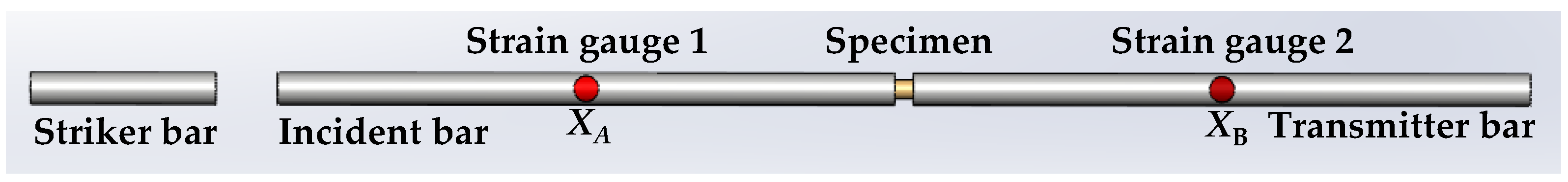
As shown in Figure 1, a typical Kolsky bar includes a striker bar, incident bar, transmitter bar, specimen, and strain gauge 1 and strain gauge 2 which are pasted at X_A of the incident bar and X_B of the transmitter bar, respectively.

Before the measurement, the specimen is placed between the incident bar and transmitter bar. Using a hammer or other tools, the strike bar is driven so that it hits the incident bar at a certain speed, thereby generating an incident wave. The specimen is deformed at high speed under the loading of the incident wave, propagates the reflected wave into the incident bar, and propagates the transmitted wave into the transmitter bar. The incident wave and the reflected wave are recorded by strain gauge 1, and the transmitted wave is recorded by strain gauge 2. The dynamic mechanical properties of the specimen can be solved from the records of these waves by theoretical calculation.

If the length of the strike bar is $L_0$, the impact velocity is $\mathsf{\nu }$, then its duration $T_{M }$ is:

$$T_M=\frac{2L_0}{C_0}$$

(1)

The magnitude of the incident pulse is:

$$A_M=\frac{{\rho }_0{C}_0\nu }{2}$$

(2)

where ${\rho }_0$ is the density of the bars. $C_0$ is the longitudinal speed of wave in the bar, and can be expressed as:

$$C_0={\left(\frac{E_0}{{\rho }_0}\right)}^{1/2}$$

(3)

where $E_{0 }$ is the elastic modulus of the bars.

If the four parameters include stress $\sigma \left(X_1,t\right)$ and $\sigma \left(X_2,t\right)$, particle velocity $\nu \left(X_1,t\right)$ and $\nu \left(X_2,t\right)$ can be measured, then the dynamic mechanical properties of the specimen can be calculated according to Formula (4)–(6).

$$\sigma \left(t\right)=\frac{A_0}{2A_S}\left[\sigma \left(X_1,t\right)+\sigma \left(X_2,t\right)\right]=\frac{A_0}{2A_S}\left[{\sigma }_I\left(X_1,t\right)+{\sigma }_R\left(X_1,t\right)+{\sigma }_T\left(X_2,t\right)\right]$$

(4)

$$\dot{\epsilon } \left(t\right)=\frac{\nu \left(X_2,t\right)-\nu \left(X_1,t\right)}{L_S}=\frac{{\nu }_T\left(X_2,t\right)-{\nu }_I\left(X_1,t\right)-{\nu }_R\left(X_1,t\right)}{L_S}$$

(5)

$$\epsilon \left(t\right)={\int }_0^t\dot{\epsilon } \left(t\right)dt=\frac{1}{L_S}{\int }_0^t\left[{\nu }_T\left(X_2,t\right)-{\nu }_I\left(X_1,t\right)-{\nu }_R\left(X_1,t\right)\right]dt$$

(6)

where $\sigma \left(t\right)$ is stress, $\dot{\epsilon } \left(t\right)$ is strain rate, $\epsilon \left(t\right)$ is strain. $L_S$ is the length of the specimen. $A_0$ and $A_S$ are the cross-sectional area of the bar and specimen, respectively. ${\sigma }_I\left(X_1,t\right)$ is incident wave, ${\mathsf{\sigma }}_R\left(X_1,t\right)$ is reflected wave, and ${\mathsf{\sigma }}_T\left(X_2,t\right)$ is transmitted wave.${\mathsf{\nu }}_I\left(X_1,t\right),{\mathsf{\nu }}_R\left(X_1,t\right)$ and ${\mathsf{\nu }}_T\left(X_2,t\right)$ are incident velocities, reflected velocities, and transmitted velocities, respectively.

According to the assumption, both the one-dimensional stress waves of the bar and the short specimen strain are evenly distributed over its length, and the three waves have the following relationship:

$${\epsilon }_I+{\epsilon }_R={\epsilon }_T$$

(7)

where ${\epsilon }_I, {\epsilon }_R \mathrm{and}{\epsilon }_T$ is strain corresponding with incident pulse, reflected pulse, and transmitted pulse, respectively.

Moreover, there is a linearly proportional relationship between strain, stress, and particle velocity [10] in the elastic region of the Kolsky bar:

$$\sigma \left(X_1,t\right)={\sigma }_I\left(X_1,t\right)+{\sigma }_R\left(X_1,t\right)=E_0\left[{\epsilon }_I\left(X_1,t\right)+{\epsilon }_R\left(X_1,t\right)\right]$$

(8)

$$\sigma \left(X_2,t\right)={\sigma }_T\left(X_2,t\right)=E_0{\epsilon }_T\left(X_2,t\right)$$

(9)

$$\nu \left(X_1,t\right)={\nu }_I\left(X_1,t\right)+{\nu }_R\left(X_1,t\right)=C_0\left[{\epsilon }_I\left(X_1,t\right)+{\epsilon }_R\left(X_1,t\right)\right]$$

(10)

$$\nu \left(X_2,t\right)={\nu }_T\left(X_2,t\right)=C_0{\epsilon }_T\left(X_2,t\right)$$

(11)

In summary, the stress, strain, and strain rate of the specimen can be expressed [11] as follows:

$$\sigma \left(t\right)=\frac{E_0}{C_0}\frac{A_0}{A_S}{\nu }_T\left(t\right)$$

(12)

$$\epsilon \left(t\right)=-\frac{2}{L_S}{\int }_0^t{\nu }_R\left(t\right)dt$$

(13)

$$\dot{\epsilon } \left(t\right)=-\frac{2}{L_S}{\nu }_R\left(t\right)$$

(14)

where ${\nu }_{T }$ and ${\nu }_{R }$ are transmitted and reflected velocities as measured, respectively.

2.2. Principle of Temporal Speckle Interferometry In-Plane Measurement

The principle of the in-plane displacement measurement used in this article is shown in Figure 2. When the object moves in the z-direction, the optical paths of both the reflected light and transmitted light change consistently [12]. Therefore, the speckle remains unchanged.

When the object moves the y-direction, one of the optical path increases $\Delta y\left(x,z,t\right)\mathit{sin}\alpha$ and the other reduces $\Delta y\left(x,z,t\right)\mathit{sin}\alpha$. Therefore, the optical path difference is as follows:

$$\delta =2\Delta y\left(x,z,t\right)\mathit{sin}\alpha$$

(15)

The phase change of the reflected light and the transmitted light is:

$$\Delta {\phi }_r=\frac{2\pi }{\lambda }\delta =\frac{4\pi }{\lambda }\Delta y\left(x,z,t\right)\mathit{sin}\alpha$$

(16)

where λ is the wavelength. α is the incident angle. Before the motion of the object, the intensity function of the speckle is:

$$I\left(x,y,t\right)=I_0\left(x,y\right)\left\{1+Vcos\left[{\Phi }_0\left(x,y\right)\right]\right\}$$

(17)

where $I_{0 }$ is the average intensity of the interference field. $V$ is the modulation visibility. ${\Phi }_0\left(x,y\right)$ is the initial phase. Hence, after the motion of the object, the intensity function of the speckle is:

$$I\left(x,y,t\right)=I_0\left(x,y\right)\left\{1+Vcos\left[{\Phi }_0\left(x,y\right)\right]\pm 4\pi \Delta y\left(x,z,t\right)\mathit{sin}\alpha /\lambda \right\}$$

(18)

where ± is the direction of the object movement.

2.3. Principle of a Kolsky Bar Based on Temporal Speckle Interferometry

As showing in Figure 3, a Kolsky bar based on in-plane displacement measurement combines two sets of in-plane displacement measuring systems and a Kolsky bar. The beam emitted from the laser is expanded and filtered by the spatial filter, and then the incident light is divided into two beams by the beam splitter. Both of them illuminate the surface of the incident bar or transmitter bar at the same angle. The back-scattered beams from the surface of the incident bar or transmitter bar form a speckle. The intensity of the speckle will change if the surface moves in the y-direction, which is captured by the detectors. The collected information is converted into a series of voltage values by the data acquisition device. By processing these voltage data with the wavelet transform and the phase unwrapping algorithm, the displacement of the incident bar or transmitter bar can be obtained according to the following formula,

$$\Delta x\left(t\right)=\frac{\lambda \Delta \Phi \left(t\right)}{4\pi sin \alpha }$$

(19)

where $\Delta \Phi \left(t\right)$ is a continuous phase based on time variation.

The velocity record is derived from the derivative of the displacement after Gaussian fitting. Therefore, the stress, strain, and strain rate of the specimen can be calculated according to the Formulae (12)–(14).

2.4. Signal Processing Procedure

Wavelet transform (WT) is a new transformation analysis method. WT inherits and develops the thought of short-time Fourier transformed localization, while overcoming shortcomings such as the window size not changing with frequency. It can automatically adapt to the requirements of time-frequency signal analysis and can focus on any detail of the signal to solve the difficult problem of the Fourier transform. It is the ideal tool for signal time-frequency analysis and processing.

The continuous wavelet coefficient [13] can be expressed as

$$W_f\left(m,n\right)={\left|m\right|}^{-1/2}\int f\left(x\right){\psi }^{*}\left(\frac{x-n}{m}\right)dx$$

(20)

where m is the scale parameter, n is the shift parameter, $f\left(x\right)$ is the signal to be analyzed, ψ(x) is the mother wavelet, and ${\psi }^{*}\left(x-n\right)/m$ is its conjugate function. The amplitude of $W_f\left(m,n\right)$ is positively correlated with the similarity of the mother wavelet and the signal [14]. In this paper, Gaussian wavelet is chosen as the mother wavelet.

The amplitudes of the light field are given by the expressions,

$$A\left(m,n\right)=\sqrt{{\left\{Im\left[W_f\left(m,n\right)\right]\right\}}^2+{\left\{Re\left[W_f\left(m,n\right)\right]\right\}}^2}$$

(21)

where $Im\left[W_f\left(m,n\right)\right]$ is the imaginary part of $W_f\left(m,n\right)$, $Re\left[W_f\left(m,n\right)\right]$ is the real part of $W_f\left(m,n\right)$.

Hence, the phase is retrieved from the following equation:

$$\Phi \left(m,n\right)=ta{n}^{-1}\left\{\frac{Im\left[W_f\left(m,n\right)\right]}{Re\left[W_f\left(m,n\right)\right]}\right\}$$

(22)

Then, through phase unwrapping, the deformation information of the measured object is obtained [15]. According to Equation (19), the object displacements can be obtained. The whole signal processing flowchart is shown in Figure 4.

3. Experiment and Results

The Kolsky bar based on in-plane displacement measurement is mainly intended to provide a new test method for the dynamic mechanical properties of small-size material samples. Therefore, the Kolsky bar is only 2 mm in diameter in the measurement system. A physical map of the guide, striker bar, incident bar, transmitter bar, and the sample is shown in Figure 5, and their sizes are shown in

Table 1. The size of each component in Kolsky bar.

Part Name	Diameter (mm)	Length (mm)
Striker bar	2	30
Incident bar	2	200
Transmitter bar	2	200
Sample	1.5	0.75
Guide	3	50

.

3.1. Verification Experiment of In-Plane Displacement Measurement Capability

According to Equations (12)–(14), the dynamic mechanical properties of the specimen depend on the velocity of the incident and transmitter bars, and the velocity is obtained by the displacement of the two bars after numerical differentiation, therefore, it is necessary to verify the displacement measurement capability of the constructed optical path. In other words, if the measurement accuracy of displacement can be guaranteed, then the dynamic mechanical properties of the sample can be considered accurate.

The verification experiment setup is shown in Figure 6. A single longitudinal mode green laser with a wavelength of 532 nm was used as the light source. The coherence length of the laser is greater than 50 m, and the beam diameter at the aperture is less than 1.5 mm. The detector (MER-030-120UC) is a color GigE Vision CCD camera (IMAVISION Company, Beijing, China) with a resolution of $656\times 492$ pixels. The pixel size is $5.6\mathsf{\mu }\mathrm{m}\times 5.6\mathsf{\mu }\mathrm{m}$, and the numerical aperture NA of camera lens is 0.052 in the image plane, which gives a speckle size in the image plane of $6.1\mathsf{\mu }\mathrm{m}$ according to Formula (23) [16],

$$\sigma =\frac{1.2\lambda }{2NA}$$

(23)

The translation stage (Thorlabs, NJ, USA) consists of the MAX302(/M) 3-Axis NanoMax Flexure Stage and three DRV3 Differential Micrometers, with a calculated fine resolution of 100 nm. The accuracy of the grating ruler is 0.1 μm.

What needs to be emphasized here is that since the entire measurement is based on the speckle, it is necessary to determine whether the optical path that we have built can form speckle interference fringes. Since the diameter of the Kolsky bar we used here is very small, the speckle interference fringes of both the incident and transmitter bar cannot be observed directly even if it does exist, two iron plates of dimensions $40\mathrm{mm}\times 30\mathrm{mm}\times 2\mathrm{mm}$ were installed in the incident and transmitter bars to verify the optical path. In Figure 7, the left part is the original structure of the experimental setup, the incident bar and the transmitter bar are placed on the support base. The right part of the figure is the structure using two iron plates to replace the incident and the transmitter bars to verify the existence of speckle interference fringes. The iron plate is fixed to the support base by two screws. In the measurement process, applying a force along the x-direction to the iron plate, the surface of the iron plate will have a slight deformation in the x-direction. The CCD camera will record the entire process of the iron plate before and after the deformation. If clear speckle interference fringes can be seen from the processed image, it is proved that the optical path to be debugged meets the measurement conditions. It is noteworthy that the position of the spot on the iron plate is the same as the position on the incident and transmitter bars; this condition has been achieved when designing the support base structure of the Kolsky bar. This ensures that the replacement between the iron plate and the bar is only for more convenient observation of the existence of speckle interference fringes, it is not related to the accuracy of the system displacement measurement capability, nor the robust position of the measuring beams.

The observation result of the speckle interference fringes is shown in Figure 8. The grey-scale maps of fringes in the incident and the transmitter bars can be observed by real-time subtraction. From this we can prove that the measurement light path meets the speckle interference measurement conditions.

After the speckle verification is completed, we replaced the iron plate with the incident and transmitter bars continue to verify the in-plane displacement measurement capability of the measurement system.

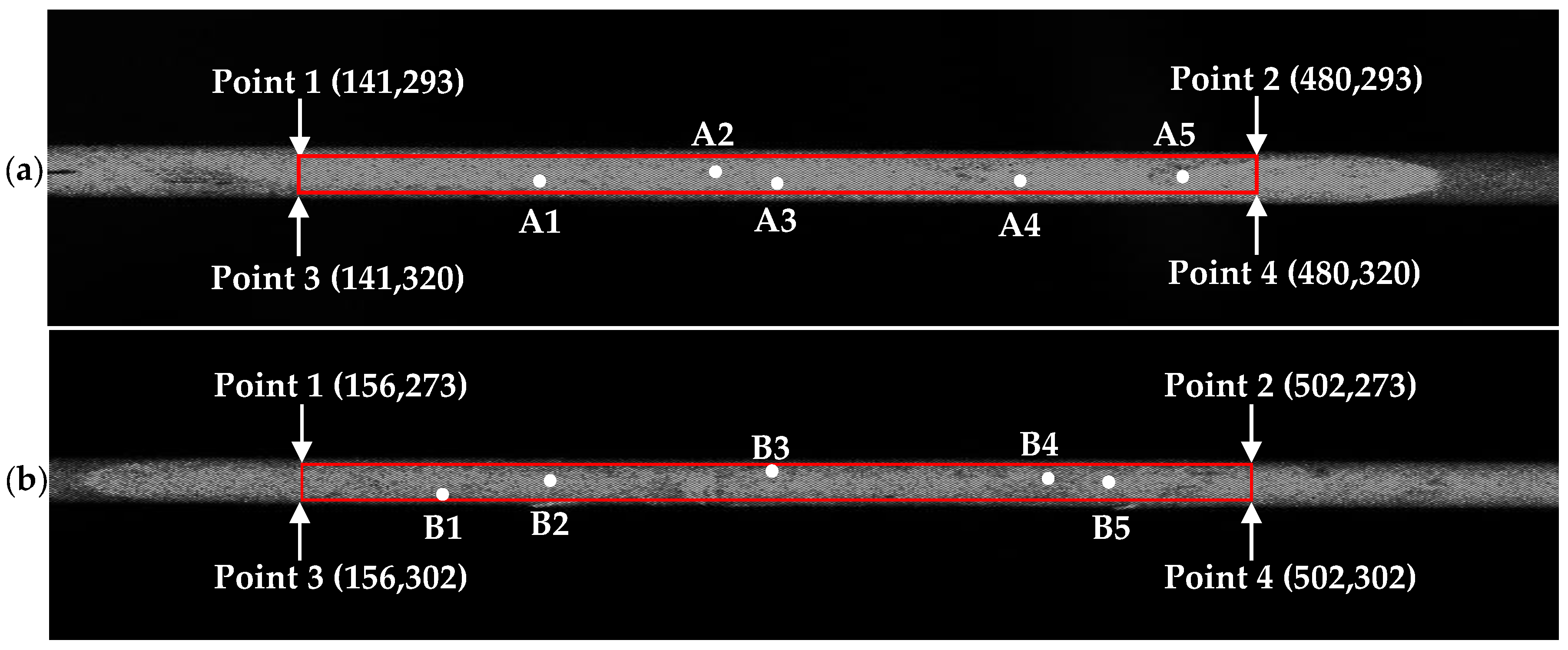
To accurately test the in-plane displacement measurement capability of the measuring system, the verification experiment was performed without a sample and the striker bar was driven with a very low velocity of a few microns per second. The translation stages push the striker bar at a slow velocity so that it strikes the incident bar at a certain velocity. The intensities of the speckles on the incident bar and transmitter bar are changed in the time domain. These changes are collected by the CCD camera. The frame rate of the CCD camera is 120 frames/s. The whole measuring time is five seconds and an arbitrary point on the position of incident bar and transmitter bar is chosen as the test point, the region of interest which is chosen arbitrarily is shown in Figure 9. At the same time, the grating ruler at the end of the transmitter bar will record the final displacement of the bar as a standard to verify the in-plane displacement detection capability of the test system.

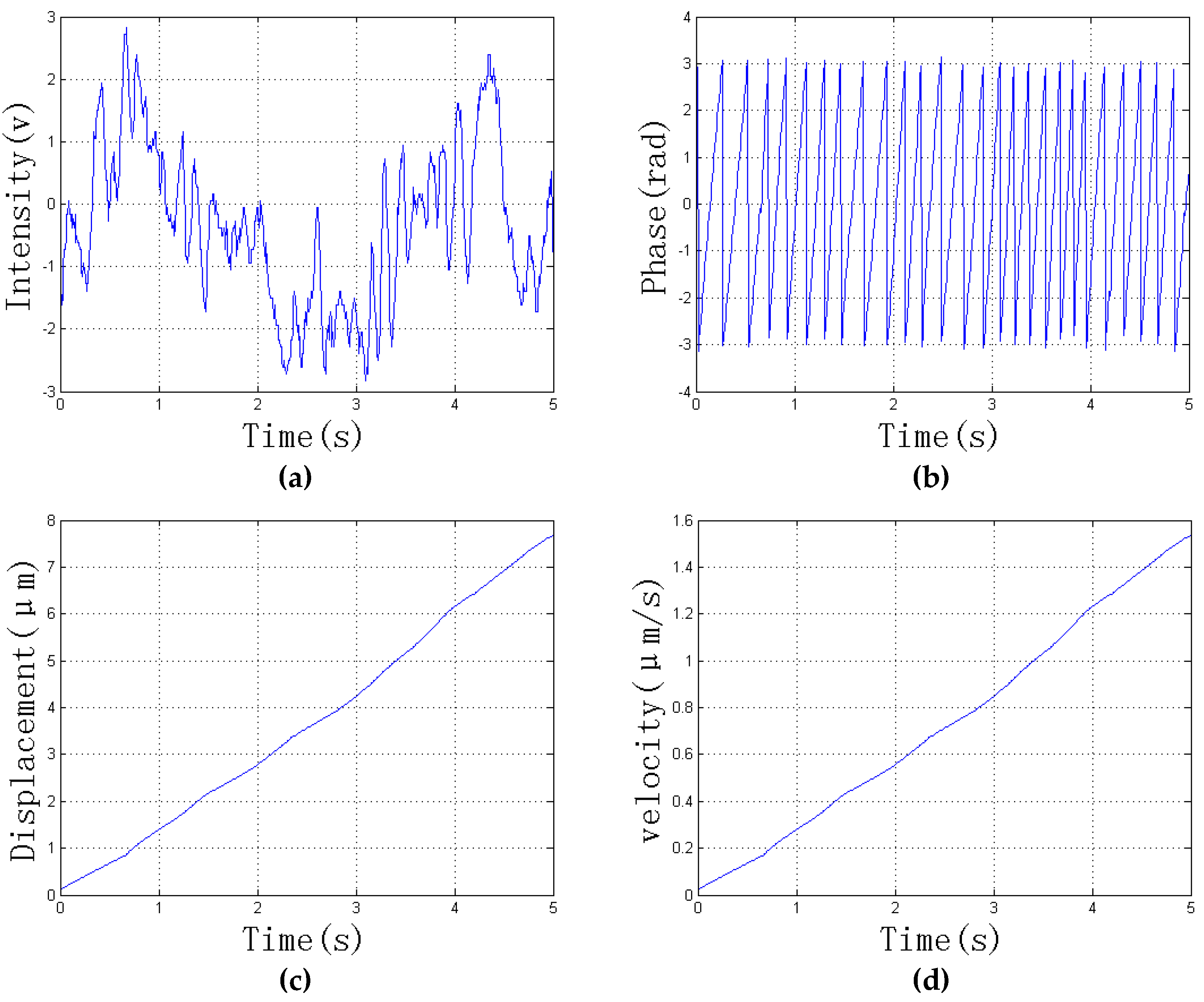
In the verification experiment, the incident angle of the incident and transmitter bars is 70 degrees and 72.5 degrees, respectively. The actual displacement of the grating ruler is 7.7 μm, and the actual average velocity of the bar is 1.54 μm/s.

The displacement of the incident bar obtained by the CCD camera is shown in Figure 10. As can be seen from the figure, the displacement processed by our algorithm is 7.68 μm and the average velocity is 1.536 μm/s. Therefore, the measured error of displacement is 0.02 μm and the measured error of velocity is 0.004 μm/s. The relative error of displacement and velocity are both 0.26%.

The displacement of the transmitter bar obtained by the CCD camera is shown in Figure 11. As can be seen from the figure, the displacement processed by our algorithm is 7.68 μm and the average velocity is 1.535 μm/s. Therefore, the measured error of displacement is 0.02 μm and the measured error of velocity is 0.005 μm/s. The relative error of displacement and velocity are 0.26% and 0.32%, respectively.

In order to verify the repeatability of the measurement system, we have also designed the system for multi-detection points processing. The measured results of two bars are shown in

Table 2. The comparison of two measurement results of multi-detection points.

Actual Value	Coordinate	Displacement (μm)			Velocity(μm/s)
		Value	Error	Relative Error	Value	Error	Relative Error
Displacement = 7.7 μm Velocity = 1.54 μm/s	A1(265,303)	7.69	0.01	0.13%	1.538	0.002	0.13%
	A2(333,296)	7.74	0.04	0.52%	1.548	0.008	0.52%
	A3(347,313)	7.71	0.01	0.13%	1.542	0.002	0.13%
	A4(419,311)	7.71	0.01	0.13%	1.542	0.002	0.13%
	A5(456,309)	7.66	0.04	0.52%	1.532	0.008	0.52%
	B1(211,302)	7.73	0.03	0.39%	1.546	0.006	0.39%
	B2(255,286)	7.65	0.05	0.65%	1.530	0.010	0.65%
	B3(380,273)	7.72	0.02	0.26%	1.544	0.004	0.26%
	B4(444,283)	7.71	0.01	0.13%	1.542	0.002	0.13%
	B5(465,294)	7.71	0.01	0.13%	1.542	0.002	0.13%

, where A1 to A5 are the points on the incident bar, and B1 to B5 are the points on the transmitter bar, as shown in Figure 9. From Table 2 we can see the displacement error of the incident bar and transmitter bar are less than 0.04 μm and 0.05 μm and the velocity error is less than 0.008 μm/s and 0.006 μm/s, respectively.

As can be seen above, the results of these verifications experiment prove that the measurement system has a very good in-plane displacement measurement capability, and the algorithm we developed can accurately calculate the information of displacement and velocity.

3.2. Experimetnal Determination of the Dynamic Mechanical Properties of Materials

The experimental setup for the determination of the dynamic mechanical properties of materials is shown in Figure 12.

The specimen described here is made of 304 L stainless steel, with diameter and thickness of 1.5 mm and 0.75 mm, respectively. The sample is held between the incident bar and the transmitter bar with butter. The pole longitudinal wave velocity $C_0$ in the bar is 4934 m/s. In order to improve the detection of changes in light intensity, here, we use a high-speed photodetector as the detector device. The high-speed photodetector is Thorlabs’ Biased Photo-detectors (DET36A/M, Thorlabs, NJ, USA), a Si biased detector covering the 350 nm to 1100 nm wavelength range and rise times as fast as 1 ns, as shown in Figure 13. A virtual oscilloscope (DSO3062AL) produced by Hantek Company (Hantek, Qindao, China) was used to collect data.

It needs to be emphasized that after the verification experiment was completed, we just removed the translation stage and the grating ruler, and the light path did not change. Therefore, the incident angle of the incident bar is still 70 degrees, and the incident angle of the transmitter bar is still 72.5 degrees.

The typical original signal for the experiment is shown in Figure 14, where the green curve is the light intensity change on the incident bar and the blue curve is the light intensity change on the transmitter bar. It can be seen from the figure that the light intensities on the two bars have a similar trend.

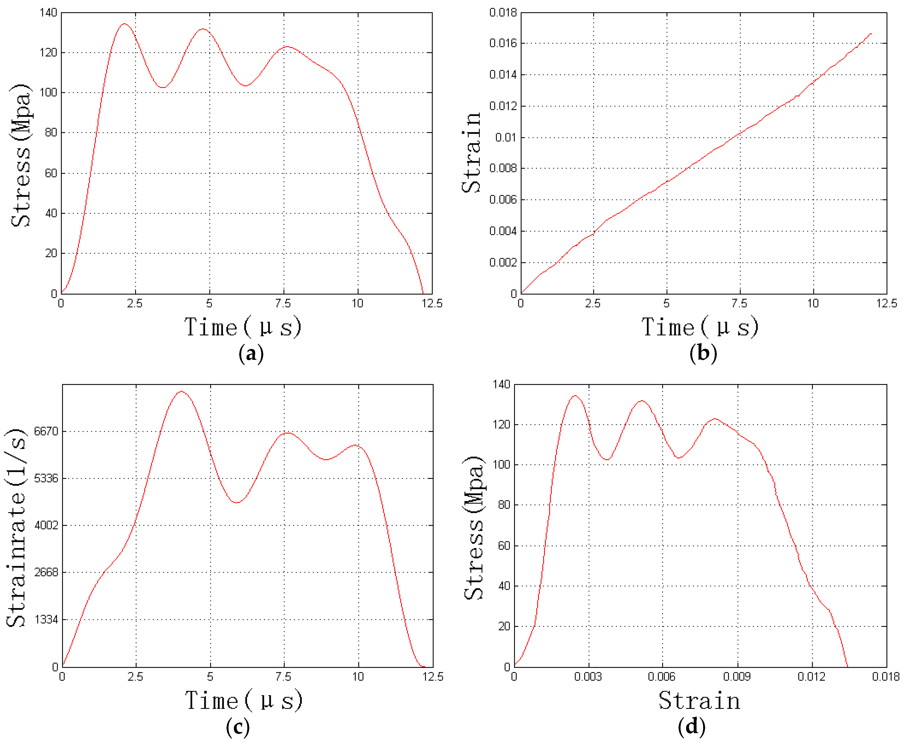
The dynamic mechanical properties of the specimen materials are shown in Figure 15.

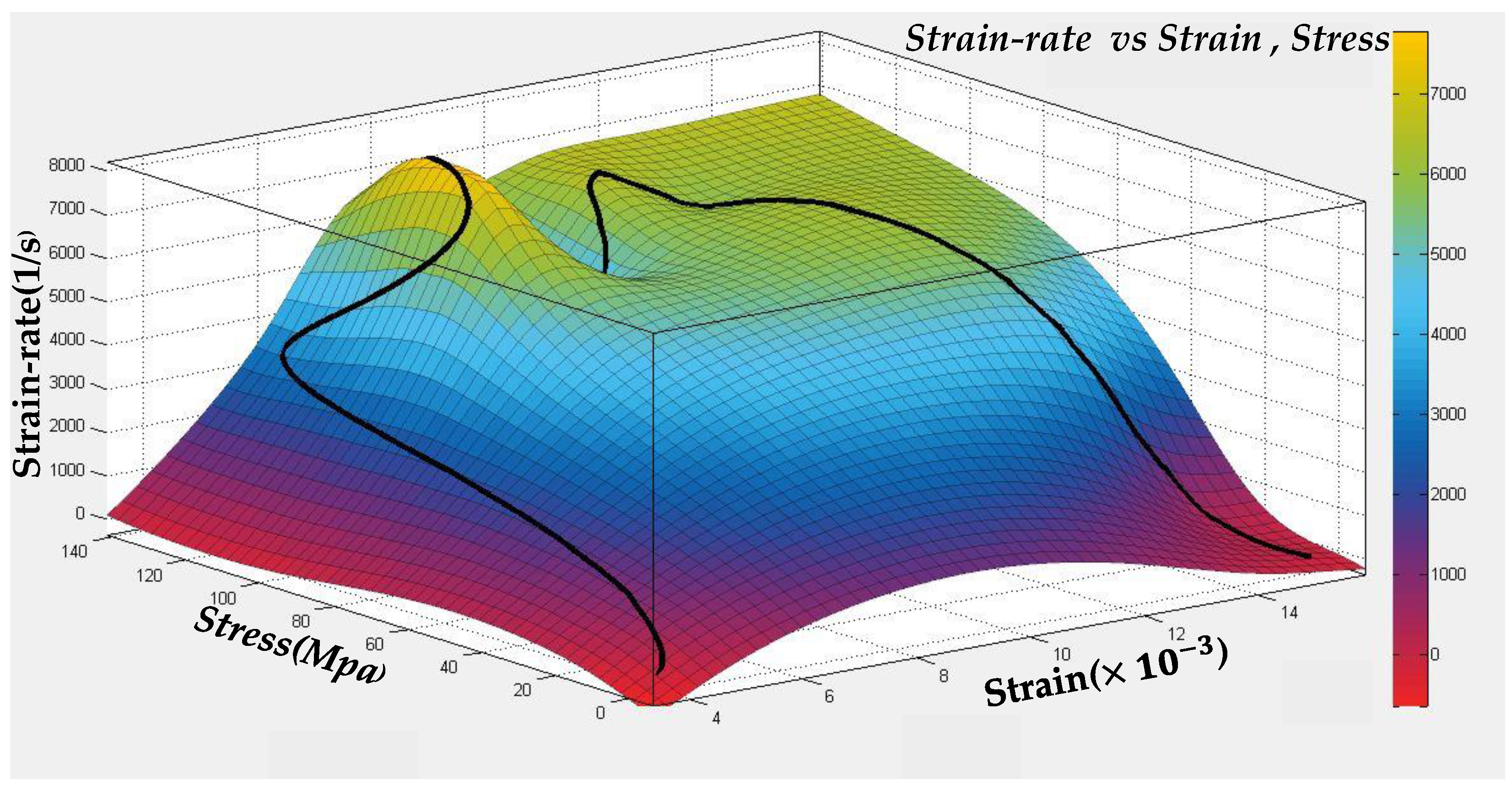
Figure 15 shows that the maximum stress applied to the specimen during the experiment was 134.21 Mpa. As the stress increased from 0 to 134.21, the maximum strain of the specimen was 0.0166, indicating that the specimen is still in the elastic phase. The strain-rate increased from 0 to 7787(1/s). Figure 16 shows the three-dimensional surface map of stress, strain, and strain rate through the interpolation fitting algorithm.

In the field of dynamic mechanics, a series of experiments to study the dynamic mechanical properties of materials are arranged according to the strain rate: medium strain rate experiments ($10~{10}^2$/s), high strain rate experiments (${10}^2~{10}^4$/s), and ultra-high strain rate experiments (${10}^4~{10}^6$/s). As can be seen from the figure, the experiment we set belongs to the second case. Note that the measurement system of Kolsky bar with temporal speckle interferometry that we give here can also be used for ultra-high strain rate experiments by reducing the diameter of the bar and increasing the velocity of striking.

4. Conclusions

With rapid development in the machinery industry and defense industry, the demand for dynamic mechanical properties of materials under higher strain rate and smaller size conditions is getting higher and higher. When the diameter of the bar is less than 3 mm, a traditional Kolsky bar is unable to provide reliable measurement because of the strain gauge and the bar cannot be reliably connected. A measurement system using a Kolsky bar with 2 mm diameter based on temporal speckle interferometry is presented in this paper. Compared with typical Kolsky bars, it can capture and process the dynamic mechanical properties of materials under higher strain rates and smaller size conditions. This method does not require any intermediate media, and has the advantages of being non-contact, real-time, and more reliable. It can be used for dynamic mechanical measurements of various solid materials, including metals, ceramics, and various composite materials, but it cannot be used for soft materials such as biological tissues. We believe that the application scope of the Kolsky bar based on temporal speckle interferometry will become more and more extensive through further research.

References

- Gama, B.A.; Lopatnikov, S.L.; Gillespie, J.W. Hopkinson bar experimental technique: A critical review. Appl. Mech. Rev. 2004, 57, 223–250. [Google Scholar] [CrossRef]
- Casem, D.; Huskins, E.; Ligda, J.; Schuster, B. A Kolsky bar for high-rate micro-compression: Preliminary results. In Dynamic Behavior of Materials; Springer International Publishing: New York, NY, USA, 2016; Volume 1, pp. 87–92. ISBN 978-3-319-22451-0. [Google Scholar]
- Avinadav, C.; Ashuach, Y.; Kreif, R. Interferometry-based Kolsky bar apparatus. Rev. Sci. Instrum. 2011, 82, 073908. [Google Scholar] [CrossRef] [PubMed]
- Priest, R.G. Analysis of fiber interferometer utilizing 3 × 3 fiber coupler. IEEE J. Quantum Electron. 1982, 18, 1601–1603. [Google Scholar] [CrossRef]
- Choma, M.A.; Yang, C.; Lzatt, J.A. Instantaneous quadrature low-coherence interferometry with 3 × 3 fiber-optic couplers. Opt. Lett. 2003, 28, 2162–2164. [Google Scholar] [CrossRef] [PubMed]
- Casem, D.T.; Zellner, M.B. Kolsky bar wave separation using a photon doppler velocimeter. Exp. Mech. 2013, 53, 1467–1473. [Google Scholar] [CrossRef]
- Casem, D.T.; Grunschel, S.E.; Schuster, B.E. Normal and transverse displacement interferometers applied to small diameter Kolsky bars. Exp. Mech. 2012, 52, 173–184. [Google Scholar] [CrossRef]
- Fu, H.; Tang, X.R.; Li, J.L.; Tan, D.W. An experimental technique of split Hopkinson pressure bar using fiber micro-displacement interferometer system for any reflector. Rev. Sci. Instrum. 2014, 85, 045120. [Google Scholar] [CrossRef] [PubMed]
- Qin, J.; Gao, Z.; Wang, X.; Yang, S. Three-dimensional continuous displacement measurement with temporal speckle pattern interferometry. Sensors 2016, 16, 2020. [Google Scholar] [CrossRef] [PubMed]
- Wang, L.L. Foundation of Stress Waves; National Defend Industry Press: Beijing, China, 2005; Volume 2, pp. 52–54. ISBN 7-118-04015-0. [Google Scholar]
- Chen, R.; Huang, S.; Xia, K.; Lu, F. A modified Kolsky bar system for testing ultrasoft materials under intermediate strain rates. Rev. Sci. Instrum. 2009, 80, 076108. [Google Scholar] [CrossRef] [PubMed]
- Gao, Z.; Deng, Y.; Duan, Y.; Zhang, Z.; Wei, C.; Chen, S.; Cui, J.; Feng, Q. Continual in-plane displacement measurement with temporal wavelet transform speckle pattern interferometry. Rev. Sci. Instrum. 2012, 83, 015107. [Google Scholar] [CrossRef] [PubMed]
- Daubechies, I. Ten lectures on wavelets (CBMS-NSF Regional Conference Series in Applied Mathematics). Soc. Ind. Appl. Math. 1992, 377. [Google Scholar] [CrossRef]
- Wang, X.; Gao, Z.; Qin, J.; Zhang, X.; Yang, S. Temporal heterodyne shearing speckle pattern interferometry. Opt. Lasers Eng. 2017, 93, 76–82. [Google Scholar] [CrossRef]
- Feng, Z.; Gao, Z.; Zhang, X.; Wang, S.; Yang, D.; Yuan, H.; Qin, J. A polarized digital shearing speckle pattern interferometry system based on temporal wavelet transformation. Rev. Sci. Instrum. 2015, 86, 61–87. [Google Scholar] [CrossRef] [PubMed]
- Svanbro, A. In-plane dynamic speckle interferometry: Comparison between a combined speckle interferometry/speckle correlation and an update of the reference image. Appl. Opt. 2004, 43, 4172. [Google Scholar] [CrossRef] [PubMed]
Figure 1.
A typical Kolsky bar.
Figure 2.
The optical path of in-plane displacement measurement.
Figure 3.
Principle of a Kolsky bar based on in-plane measurement; 1 and 8 are lasers; 2 and 9 are spatial filters; 3 and 10 are beam splitters; 4, 5, 11, and 12 are reflectors; 6 and 13 are detectors; 7 and 14 are computers; 15 is an oscilloscope; 16 and 17 are optical fibers; 18 and 19 are fiber detectors; 20 is the striker bar; 21 is the guide; 22 is the incident bar; 23 is the specimen; 24 is the transmitter bar; 25 is the support frame.
Figure 4.
Signal processing flowchart.
Figure 5.
Physical map of each component in Kolsky bar.
Figure 6.
Verification experiment setup: 1 and 18 are green lasers; 2 and 16 are beam lifters; 3 and 17 are spatial filters; 4 and 13 are beam splitters; 5 is a grating ruler; 6, 9, 11, and 15 are reflectors; 7 and 14 are CCD; 8 is the trigger device; 10 is the translation stage; 12 is an oscilloscope; 19 is the SHPB device.
Figure 7.
Iron plate instead of incident bar and transmitter bar: (a) Original structure; (b) Replacement structure.
Figure 8.
Speckle verification results from the position of incident bar and the transmitter bar: (a) Speckle on the incident bar; (b) Speckle on the transmitter bar.
Figure 9.
The region of interest: (a) incident bar; (b) transmitter bar.
Figure 10.
The in-plane displacement of the incident bar: (a) the intensity distribution over time; (b) the discontinuous phase map obtained by wavelet transformation; (c) the measured displacement over time; (d) average speed.
Figure 11.
The in-plane displacement of the transmitter bar: (a) the intensity distribution over time; (b) the discontinuous phase map obtained by wavelet transformation; (c) the measured displacement over time; (d) average speed.
Figure 12.
Dynamic mechanical properties of materials experimental setup: 1 and 18 are green lasers; 2 and 16 are beam lifters; 3 and 17 are spatial filters; 4 and 13 are beam splitters; 5 is a baffle; 6, 10, 11 and 15 are reflectors; 7 and 14 are point detectors; 8 is a virtual oscilloscope; 9 is the trigger device; 12 is an oscilloscope; 19 is the SHPB device.
Figure 13.
Photodetector.
Figure 14.
Original light intensity signal: (a) intensity of incident bar; (b) intensity of transmitter bar.
Figure 15.
Dynamic mechanical properties of the specimen: (a) stress curve; (b) strain curve; (c) strain rate curve; (d) stress–strain curve.
Figure 16.
Three-dimensional surface map of stress, strain, and strain rate.