Leader–Follower Formation Maneuvers for Multi-Robot Systems via Derivative and Integral Terminal Sliding Mode

School of Control and Computer Engineering, North China Electric Power University, Beijing 102206, China
*
Author to whom correspondence should be addressed.
Appl. Sci. 2018, 8(7), 1045; https://doi.org/10.3390/app8071045
Submission received: 10 May 2018
/
Revised: 3 June 2018
/
Accepted: 11 June 2018
/
Published: 27 June 2018
(This article belongs to the Special Issue Swarm Robotics)
Abstract
:Featured Application
The presented control design can enrich the multi-robot technologies and can benefit the coordination of multi-robot systems.
Abstract
This paper investigates the formation problem of multiple robots based on the leader–follower mechanism. At first, the dynamics of such a leader–follower framework are modeled. The input–output equations are depicted by calculating the relative degree of a leader–follower formation system. Furthermore, the derivative and integral terminal sliding mode controller is designed based on the relative degree. Since the formation system suffers from uncertainties, the nonlinear disturbance observer is adopted to deal with the uncertainties. The stability of the closed-loop control system is proven in the sense of Lyapunov. Finally, some numerical simulations are displayed to verify the feasibility and effectiveness by the designed controller and observer.
1. Introduction
In recent years, the coordination control scheme of multiple robots has drawn considerable attention in various fields [1]. Multiple robots can be applied in many dangerous places to free the human being, including the earthquake rescue, the warehouse translations, and some tasks at nuclear power plants. A multi-robot system can be treated as a coupling network of some robots, where the robots communicate with each other to achieve some complex duties [2,3]. Various investigations have been explored to achieve the coordination control of multiple robots. These investigations can be roughly classified into leader–follower formations [4,5,6,7,8], virtual structure mechanisms [9,10,11,12], graph-based approaches [13,14], and behavior-based methods [15,16].
The leader–follower formations are attractive in the coordination control of multi-robot systems. Partly, such formations benefit multiple robots because the formations can have guaranteed formation stability via control design [17]. The basic control idea of the leader–follower mechanism is that multiple robots are divided into several leader–follower pairs. In the leader–follower mechanism, all follower robots share the same leader. In each pair, the leader robot moves along the predefined trajectory, while the follower robots track the leader with desired relative distance and angle. In the leader–follower system of multiple robots, only partial followers can obtain the state of the leader, and the interaction between follower robots and leader robot is local [18]. Many control methods have been applied in the leader–follower multi-robot systems, such as sliding mode control (SMC) based on nonlinear disturbance observer [18], SMC [19], second-order SMC [20], adaptive control [21,22], predictive control [23], integral terminal SMC [24], and terminal SMC [25].
In actuality, it is unavoidable for any robots to be affected by uncertainties such as external disturbances, unmodeled dynamics, and parameter perturbations [26]. The dynamics of multi-robot systems becomes uncertain, due to these uncertainties [27]. These uncertainties can be categorized into unmatched uncertainties and matched uncertainties [28]. However, the SMC method, as a strong robust tool, has invariant nature to the matched uncertainties when an SMC system enters into the sliding mode. Unfortunately, the effects of unmatched uncertainties cannot be suppressed by the SMC methods [29]. The unmatched uncertainties can challenge the performance of the SMC system seriously. The characteristic of terminal SMC (T-SMC) has its nonlinear sliding surface. Compared with those traditional SMC approaches, the T-SMC method has faster convergence speed and higher accuracy. However, the T-SMC method has the singular problem due to its fractional function. Therefore, the derivative and integral T-SMC (DIT-SMC) method is proposed [30]. The DIT-SMC method is of merit. Due to the existence of the integral term, the sliding mode of the DIT-SMC method starts on the derivative and integral terminal sliding mode surface. Moreover, the DIT-SMC method can guarantee the exact estimation of finite error convergence time, and resolve the singular problem of the T-SMC. On the other hand, the derivative term of the DIT-SMC method can reduce the nonlinear effects to the stability of a DIT-SMC system.
In the previous works [21,22,23,24,25,26,27,28,29,30], the assumption that the uncertainties have a known boundary is assumed. Concerning the formation maneuvers of multi-robot systems, the assumption is not mild. In fact, the boundary of uncertainties in multiple robots is hard to be known exactly in advance. In case of the lack of the important information, several serious problems may be raised in reality, for example, the decrease of the formation robustness, the deterioration of the formation performance, as far as the deficiency of the formation stability. In order to resolve the problem of the uncertainties, the nonlinear disturbance observer is adopted. The unknown unmatched uncertainties are estimated by the nonlinear disturbance observer. The technique of nonlinear disturbance observer (NDOB) can handle the unmatched uncertainties problem and improve the robustness of the formation control system.
This paper deals with the formation problem of multiple robots with uncertainties. The control scheme combining derivative and integral terminal sliding mode and nonlinear disturbance observer is investigated. The derivative and integral terminal sliding mode method allows the system start on the sliding surface. The reaching time of sliding surface is eliminated. The matched uncertainties in formation system are suppressed by the DIT-SMC method. Under the mild assumption that the uncertainties have an unknown boundary, the NDOB is designed to estimate the unmatched uncertainties in the formation system. The estimate errors will converge to zero in the limited time by setting the parameter of NDOB. In the sense of Lyapunov, the system stability is guaranteed in spite of uncertainties. Finally, some numerical simulations are displayed to illustrate the feasibility and effectiveness.
2. Problem Formulation
2.1. Modeling of Single Robot
Shown by Figure 1, a unicycle-like robot is taken into account. The robot is round, with r in radius, and has two parallel wheels controlled independently by two DC motors. Because the robot is capable of simultaneous arbitrary rotation and translation in the horizontal plane, a three dimensional vector q = [x, y, θ]T is used to describe the robot. In Figure 1, (x, y) represents the translational coordinates of the robot, and is the center of the robot. The rotational coordinate is depicted by the variable θ.
There are n robots in the formation system of multi-robot. Provided the pure rolling and no-slipping condition, the ideal dynamic models of the nth robot are described by
where vn, ωn are the linear velocities and angular velocities, respectively.
Differentiate (1) with respect to time t. Considering the parameter fluctuations, model uncertainties, and external disturbances, such as slipping and skidding effects in the formation system, the dynamic model of the nth robot is obtained by
where un = [αn βn]T is the control input of nth robot. αn, βn are the acceleration and angular acceleration respectively, which are described by αn = Fn/mn, βn = τn/Jn. Here, Fn, mn, τn, and Jn donate the force, the nominal mass, the torque of the robot, and the nominal moment of inertia, respectively. ∆n represents the parameter fluctuations, written by
where , represent the variant on the mass and the inertia. is described by [πnx πny πnθ]T, meaning the uncertainties and external disturbances in the lumped model.
2.2. Leader–Follower Formation Framework
In this section, the kinematics model of the leader–follower formation system is given. The leader–follower formation mechanism is displayed in Figure 2. In the leader–follower formation system, there is a leader robot, and others are selected as follower robots. The ith robot is set as the leader robot, and the kth robot is picked up as the representative of all follower robots. The relative distance lik and relative bearing angle ϕik between the leader robot and follower robot are defined in Figure 2. The relative distance lik means the distance between the center of the leader robot ith and the front castor of the follower robot kth, described by
Here, (xi, yi) denotes the center of the leader robot i, and represents the caster position of the follower robot k. The calculation of , has the following form
Here, r is the radius of the round robot, and (xk, yk) denotes the center of the follower robot k. Simultaneously, is formulated by
Here, θi denotes the orientation angle of the leader robot i, .
In this paper, the derivative and integral terminal sliding mode controller is designed so that the follower robots can follow the leader robot with desired relative distance and angler. Therefore, the following conditions are satisfied: The collisions between the robots are avoided. There is no communication delay between the leader robot and the follower robot. Each follower robot knows its position, velocity, and corresponding information of the leader robot.
According to leader–follower formation mechanism, the robots move along a specified trajectory with desired relative distance and bearing angle. It is necessary to shape the dynamics of the leader–follower formation system. Differentiate (3) and (5) twice with the respect to time t, and substitute (2) into the second derivative of (3) and (5). Define the state variable xik = [x1 x2 x3 x4]T, where , , , . The dynamic model of the formation system has the form of
Here, is a 2 × 2 matrix whose columns are smooth vector fields . is the output equation of formation system. Here,
Aik, Bik,1, Bik,2, h(xik) are described by
Here, , denotes the uncertainties of the leader–follower formation system (6), written by
F1, F2, P1, P2 are depicted respectively by
2.3. Control Problem Formulation
Considering the dynamic mode (6) of the leader–follower formation system, a relative-degree is calculated by
Here, rK (K = 1, 2) is the smallest integer so that the least one of the control inputs appears in (K = 1, 2), then
Here, r1 = r2 = 2, m = 2. , are lie derivatives. Further, the input–output dynamic equation is depicted by
Here, , . Here, I3, I4 are 2 × 2 matrices, ui is the control input of ith robot, and other matrices are described by
Hypothesis 1.
has the normal part Gik and nonlinear part Gik∆k, and meets the following in equation
Here, δik > 1, , I is the 2 × 2 square matrix, denotes the desired state vector in (6).
Remark 1.
Gik∆kuk is the matched uncertainties in (13), meaning the parameter fluctuations of the follower robot k. The term dik depicts the unmatched uncertainties in the leader–follower formation system, and consists of three parts. Due to the formation, framework (13) is applied to the follower robot, and the information of leader robot ui can't be matched.
The terms , denote the model uncertainties and external disturbances caused by slipping, friction, and obstacles etc., which are also hard to be matched.
3. Control Design
Due to the inherent characteristics of centralization, the scheme mainly depends on the leader robots and exists as the “single point of failure” problem. In order to develop derivative and integral terminal sliding mode approach to coordinate the leader robot i and follower robot k, a recursive structure of the terminal sliding function for high relative-degree MIMO systems (with r1, r2 > 1) is designed as
where , . γik,1, γik,2, λik,1, λik,2 are all positive constants. pKj > qKj, here K, j = 1, 2. pKj and qKj are all odd positive constants.
Theorem 1.
Considering the derivative and integral terminal sliding mode surface Sik(t) with the fractional function, the state error of formation system can reach the equilibrium point e = 0 at the limited time
Here, t1K (K = 1, 2) is the reaching time of terminal slide mode eD1K.
Proof.
From (17), the sliding mode sik starts on t = 0. Then, the equations and can always hold true by control design. Subsequently, substituting , into and , respectively, yields
□
The converge time of sliding mode and can obtained by solving (19).
In sliding mode sik = 0, , and can always hold true. Therefore, the reaching time of and are the same as the convergence time of and , respectively. When , and will converge to zero successfully. At t = t1K (K = 1, 2), the and are formulated by
Solving (21), the , from , to will spend the time
Since the sliding mode sik = 0 consists of the derivative term and integral term, the time TK spending from sik.K = 0 (K = 1, 2) to eik,K = 0 (K = 1, 2) is the summation of the two terms. Since the fact that each sliding mode sik,1, sik,2 is independent, the time spent for equilibrium point is the max of the TK.
Hypothesis 2.
. It means that the unmatched uncertainties of formation system (13) have a boundary.
Differentiating the sliding function sik with the respect to time t, and substituting (13) into the derivative of sik can get
where denotes the desired distance and angle between the leader robot and follower robots. . and are depicted respectively by
The derivative and integral terminal sliding mode control law is set as
where , keik, ηik are all the positive constant set by designer. is the upper bound of the unmatched uncertainties.
, (K = 1, 2) are written as
Here, , χik and keik meet the following conditions
Substitute the control law (25) into (23), considering the conditions (26). Then, can be guaranteed when holds true. However, apart from Hypothesis 2, the unmatched uncertainties in (13) are unknown, which means that the upper bound is also unknown. Therefore, it cannot select an appropriate parameter to guarantee . Therefore, the stability of control system cannot be guaranteed.
DIT-SMC Design Based NDOB
In order to resolve the above problem, the nonlinear disturbance is proposed to estimate the uncertainties in the leader–follower formation system (13). At first, the following assumption is taken into account.
Hypothesis 3.
The unmatched uncertainties possess a slow change rate, meaning that , where.
Considering the formation dynamic model (6), the nonlinear disturbance observer is formulated by
Here , , are the state vector of nonlinear disturbance observer, the observer gain matrix set by designer, and the estimated value of unmatched uncertainties respectively.
Define the estimate error vector as
Differentiate edik with respect to time t and take the Hypothesis 3 into account. Furthermore, the dynamics of is presented as
The solution of (30) is , which indicates the estimate error will exponentially converge to zero as t → ∞ if is set as a positive constant. Here, is the initial state of .
Considering input–output dynamics (13) and observer (29), the control law based on NDOB is determined by
Theorem 2.
Consider the dynamic model of leader–follower formation system (6), take the assumption 1, 2, 3, 4 into account, adopt the input–output model (13), design the derivative and integral terminal sliding mode surface (17) and nonlinear disturbance observer (29). If the derivative and integral terminal control law is set as (31), the leader–follower formation system with unmatched uncertainties is asymptotically stable when .
Proof.
Selecting the Lyapunov function as , differentiating Vik with the respect to time t and substituting the into the derivative of Vik yields
Here, . Since p1K > 0, q1K > 0, p2K > 0, q2K > 0, p1K > q1K, p2k > q2K exist in the controller, and hold true for all , . According to the Hypothesis 1, (27), the second term and the third term can be deduced by
□
In (33), the condition can be picked up so that the holds true.
The first term of has the following form of
, can be selected in the control design in order to ensure is held true.
can be picked up by deducing from (32)–(34). That illustrates the control law can asymptotically stabilize the leader–follower formation system by the derivative and integral terminal sliding mode. Therefore, the follower robots can trace the leader robot with the desired distance and angle steadily. The characteristics of DIT-SMC method are as follows: (1) the convergence time Tk can be adjusted by the parameters of the control law; (2) the formation system starts on the derivative and integral terminal sliding surface; (3) the singular problem of T-SMC is avoided; (4) the derivative term can weaken the nonlinear effect.
In (31), the parameter must be assigned as a conservative value to guarantee the formation system stability. From (30), edik can be exponentially convergent to 02×1 by selecting Lik, meaning that κik can be very small. Even if κik is assigned from a conservative perspective, its value may not be very large. That illustrates the DIT-SMC based NDOB control law protects the formation from the high switching frequency problem, and can substantially alleviate the chattering problem.
4. Numerical Simulations
Considering the dynamic model of the leader–follower formation system (6), the derivative and integral terminal sliding mode controller is proposed. There are three robots in the leader–follower framework, where the two follower robots track along with the leader robot. The radius of each robot is 0.05 m. The parameter fluctuations in formation system are determined by
where i = 1 denotes the leader robot, and k = 2, 3 represent the two follower robots. The uncertainties and external disturbances in lumped model (6) are depicted by
The parameters in control design are set as γ12,1 = γ12,2 = γ13,1 = γ13,2 = 4, λ12,1 = λ12,2 = λ13,1 = λ13,2 = 1, p11 = p12 = 9, q11 = q12 = 7, q21 = 3, p21 = 5, q22 = 7, p22 = 9, ke12 = ke13 = 20, ε12 = ε13 = 4, k12 = k13 = 2, δ12 = δ13 = 4, η12 = η13 = 0.2.
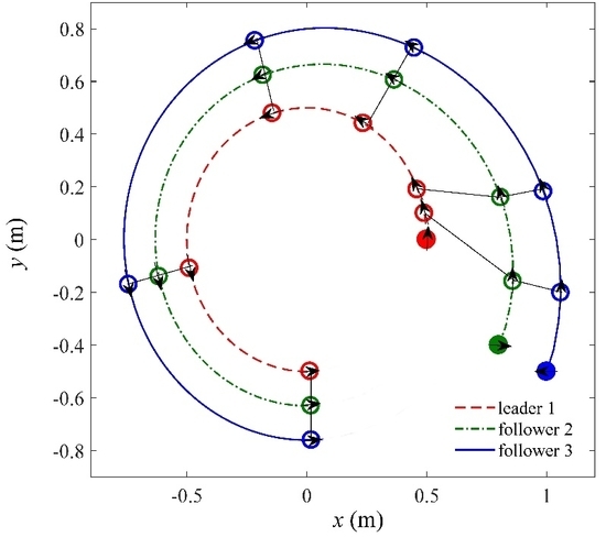
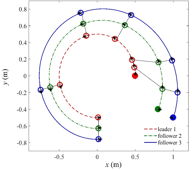
Considering the circle trajectory for the formation system in Figure 3, the initial state vector is respectively set as = [0.5 m 0 m/s−1 3.2π/4 rad 0 rad/s], = [0.707 m 0 m/s−1 3π/4 rad 0 rad/s]. The desired state vectors are respectively designated as = [0.13 m 0 m/s−1 π/2 rad 0 rad/s], = [0.26 m 0 m/s−1 π/2 rad 0 rad/s]. The desired linear and angular velocities of leader robot are designated as , . The simulation results are shown in Figure 4, Figure 5 and Figure 6.
Figure 3 displays the moving curve of the formation system, which shows the robots are in a line while moving along the circular trajectory. In Figure 3, the solid point denotes the initial position of the formation robots. The arrows are the moving directions of the three robots. It is seen form the Figure 3 that the follower can track the leader robot with the desired distance and angle, while the leader robot tracks the circular trajectory.
In order to provide more insight into the system performance, some comparisons among the SMC method, the second-order SMC, the SMC based NDOB [18], and the DIT-SMC based NDOB are shown in Figure 4, Figure 5 and Figure 6. The parameters of the sole SMC and SMC based NDOB method are presented in [18], and the parameters of second-order SMC are same as paper [20]. The relative distance and relative angular between the leader robot 1 and the two follower robots 2, 3 are displayed in Figure 4. Comparing with the SMC method, the second-order SMC and the SMC based NDOB, the DIT-SMC based NDOB method has shorter convergence time and smoother than the other methods.
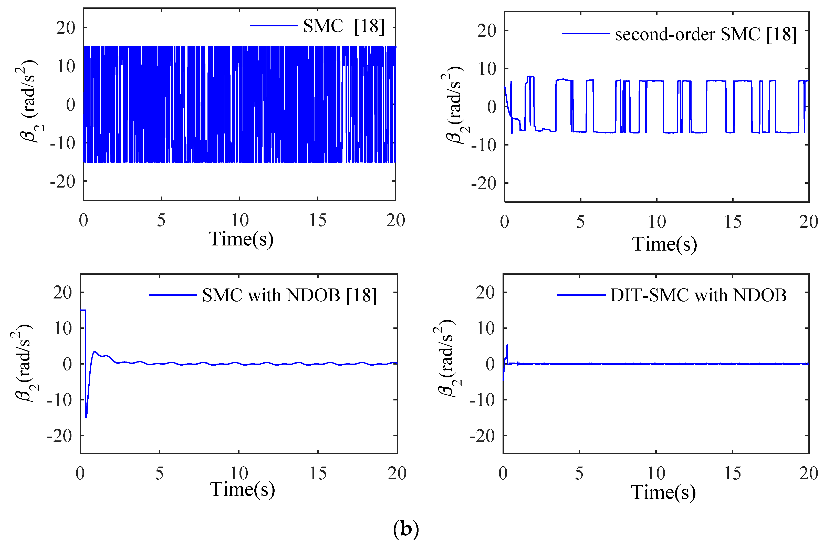
Figure 5 denotes the control input of follower robot 2 using different control method. In Figure 5a, the acceleration of follower robot 2 are shown, while the angular accelerations of follower robot 2 are displayed in Figure 5b. From Figure 5a,b, the control input of DIT-SMC based NDOB is smoother than other control methods, which denotes the acceleration and angular acceleration are more stable.
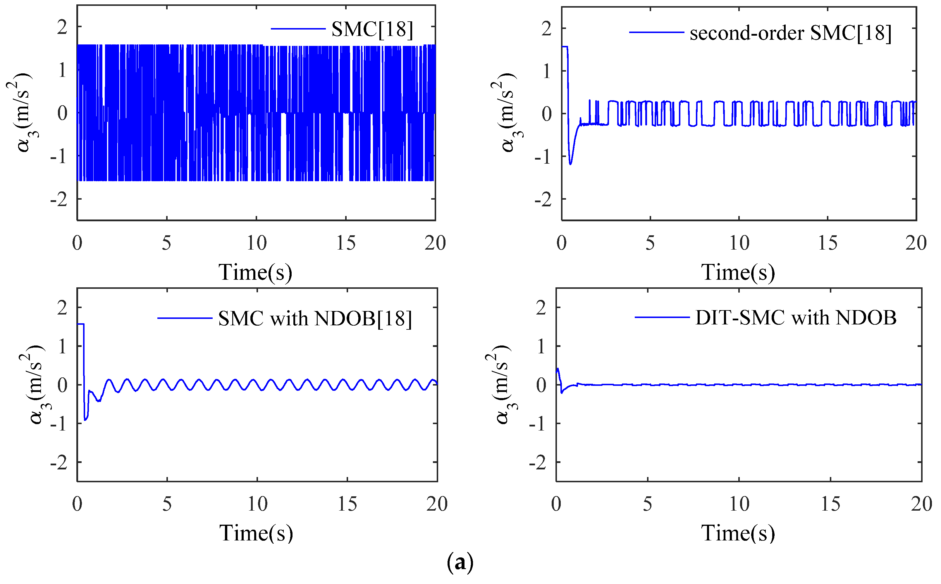
The control inputs of follower robot 3 are shown in the Figure 6, which denotes the acceleration and angular acceleration of follower robot 3. The accelerations of follower robot of follower robot using the three control methods are displayed in Figure 6a, while the angular acceleration using three methods are shown in Figure 6b. From Figure 5 and Figure 6, the combination of the DIT-SMC and NDOB can benefit the decrease of the chattering phenomenon that is an inherent drawback of the SMC methodology.
Figure 7 denotes the sliding mode vectors of two follower robots. As proven in the Theorem 1, the reaching time of sliding surface will be eliminated, and the error of formation system will reach to the equilibrium point in the finite time. From Figure 7, the formation system can enter the sliding mode in the beginning, which can guarantee the system stability.
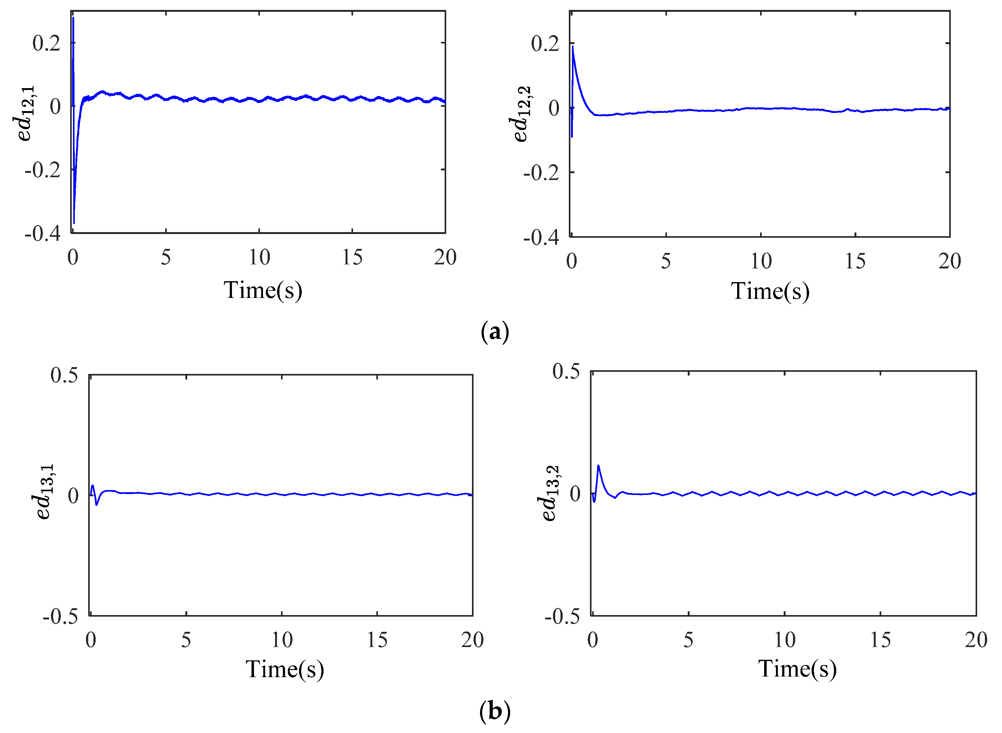
Figure 8 illustrates the elements of the estimate-error vectors, where the vectors ed12 are shown in the Figure 8a, and the vectors ed13 are shown in the Figure 8b. From the Figure 8, the estimate-error can converge to zero in the finite time. The value of estimate-error is max when t = 0, that is, the maximum is less than 0.5. However, the value of kik is selected 2. Therefore, the system stability can be guaranteed.
5. Conclusions
This paper investigates the formation control problem of multi-robot systems based on the leader–follower mechanism. The leader–follower formation system becomes uncertain because of some adverse effects, such as the parameter fluctuations, external disturbances, and so on. In order to estimate the uncertainties, a control scheme, combining the DIT-SMC and the NDOB, is proposed under the assumption that the uncertainties have an unknown boundary. The stability of the control scheme is proven in the light of Lyapunov theorem. Some simulation results are demonstrated to show the feasibility of the control scheme.
Author Contributions
Methodology, D.Q.; Software, Y.X.; D.Q. contributed theoretical analysis and Y.X. performed the numerical experiments.
Funding
The work is supported by the National Natural Science Foundation of China (61473176) and the Fundamental Research Funds for the Central Universities (2018MS025).
Conflicts of Interest
The authors declare no conflict of interest.
References
- Dai, Y.; Kim, Y.; Wee, S.; Lee, D.; Lee, S. Symmetric caging formation for convex polygonal object transportation by multiple mobile robots based on fuzzy sliding mode control. ISA Trans. 2016, 60, 321–332. [Google Scholar] [CrossRef] [PubMed]
- Li, C.D.; Gao, J.L.; Yi, J.Q.; Zhang, G.Q. Analysis and design of functionally weighted single-input-rule-modules connected fuzzy inference systems. IEEE Trans. Fuzzy Syst. 2018, 26, 56–71. [Google Scholar] [CrossRef]
- Qian, D.W.; Li, C.D. Formation control for uncertain multiple robots by adaptive integral sliding mode. J. Intell. Fuzzy Syst. 2016, 31, 3021–3028. [Google Scholar] [CrossRef]
- Loria, A.; Dasdemir, J.; Jarquin, N.A. Leader-follower formation and tracking control of mobile robots along straight paths. IEEE Trans. Control Syst. Technol. 2016, 24, 727–732. [Google Scholar] [CrossRef]
- Li, C.D.; Ding, Z.X.; Zhao, D.B.; Yi, J.Q.; Zhang, G.Q. Building energy consumption prediction: An extreme deep learning approach. Energies 2017, 10, 1525. [Google Scholar] [CrossRef]
- Li, C.D.; Ding, Z.X.; Yi, J.Q.; Lv, Y.S.; Zhang, G.Q. Deep belief network based hybrid model for building energy consumption prediction. Energies 2018, 11, 242. [Google Scholar] [CrossRef]
- Biglarbegian, M. A novel robust leader-following control design for mobile robots. J. Intell. Robot. Syst. 2013, 71, 391–402. [Google Scholar] [CrossRef]
- Dai, Y.; Lee, S.G. The leader-follower formation control of nonholonomic mobile robots. Int. J. Control Autom. Syst. 2012, 10, 350–361. [Google Scholar] [CrossRef]
- Mehrjerdi, H.; Ghommam, J.; Saad, M. Nonlinear coordination control for a group of mobile robots using a virtual structure. Mechatronics 2011, 21, 1147–1155. [Google Scholar] [CrossRef]
- Li, J.; Wang, J.; Pan, Q.; Duan, P.; Sang, H.; Gao, K.; Xue, Y. A hybrid artificial bee colony for optimizing a reverse logistics network system. Soft Comput. 2017, 21, 6001–6018. [Google Scholar] [CrossRef]
- Qian, D.W.; Tong, S.W.; Li, C.D. Observer-based leader-following formation control of uncertain multiple agents by integral sliding mode. Bull. Pol. Acad. Sci. Tech. Sci. 2017, 65, 35–44. [Google Scholar] [CrossRef] [Green Version]
- Qian, D.W.; Tong, S.W.; Lee, S.G. Fuzzy-Logic-based control of payloads subjected to double-pendulum motion in overhead cranes. Autom. Constr. 2016, 65, 133–143. [Google Scholar] [CrossRef]
- Fax, J.A.; Murray, R.M. Information flow and cooperative control of vehicle formations. IEEE Trans. Autom. Control 2004, 49, 1465–1476. [Google Scholar] [CrossRef]
- Lin, Z.Y.; Francis, B.; Maggiore, M. Necessary and sufficient graphical conditions for formation control of unicycles. IEEE Trans. Autom. Control 2005, 50, 121–127. [Google Scholar] [Green Version]
- Lawton, J.T.; Beard, R.W.; Young, B.J. A decentralized approach to formation maneuvers. IEEE Trans. Robot. Autom. 2003, 19, 933–941. [Google Scholar] [CrossRef] [Green Version]
- Liang, H.Z.; Sun, Z.W.; Wang, J.Y. Finite-time attitude synchronization controllers design for spacecraft formations via behaviour based approach. Proc. Inst. Mech. Eng. Part G J. Aerosp. Eng. 2013, 227, 1737–1753. [Google Scholar] [CrossRef]
- Li, J.; Sang, H.; Han, Y.; Wang, C.; Gao, K. Efficient multi-objective optimization algorithm for hybrid flow shop scheduling problems with setup energy consumptions. J. Clean. Prod. 2018, 181, 584–598. [Google Scholar] [CrossRef]
- Qian, D.W.; Tong, S.W.; Li, C.D. Leader-following formation control of multiple robots with uncertainties through sliding mode and nonlinear disturbance observer. ETRI J. 2016, 38, 1008–1018. [Google Scholar] [CrossRef]
- Park, B.S.; Park, J.B.; Choi, Y.H. Robust formation control of electrically driven nonholonomic mobile robots via sliding mode technique. Int. J. Control Autom. Syst. 2011, 9, 888–894. [Google Scholar] [CrossRef]
- Defoort, M.; Floquet, T.; Kokosy, A.; Perruquetti, W. Sliding-mode formation control for cooperative autonomous mobile robots. IEEE Trans. Ind. Electron. 2008, 55, 3944–3953. [Google Scholar] [CrossRef]
- Chen, X.; Jia, Y. Adaptive Leader-follower formation control of non-holonomic mobile robots using active vision. IET Control Theory Appl. 2014, 9, 1302–1311. [Google Scholar] [CrossRef]
- Park, B.S.; Park, J.B.; Choi, Y.H. Adaptive formation control of electrically driven non-holonomic mobile robots with Limited Information. IEEE Trans. Syst. Man Cybern. B Cybern. 2011, 41, 1061–1075. [Google Scholar] [CrossRef] [PubMed]
- Howard, T. Model-predictive motion planning several key developments for autonomous mobile robots. IEEE Robot Autom. Mag. 2014, 21, 64–73. [Google Scholar] [CrossRef]
- Muhammad, A.; Muhammad, J.K.; Attaullah, Y.M. Integral terminal sliding mode formation control of non-holonomic robots using leader follower approach. Robotica 2017, 35, 1473–1487. [Google Scholar]
- Nair, R.R.; Karki, H.; Shukla, A.; Behera, L.; Jamshidi, M. Fault-tolerant formation control of nonholonomic robots using fast adaptive gain nonsingular terminal sliding mode control. IEEE Syst. J. 2018. [Google Scholar] [CrossRef]
- Qian, D.W.; Tong, S.W.; Liu, H.; Liu, X.J. Load frequency control by neural-network-based integral sliding mode for nonlinear power systems with wind turbines. Neurocomputing 2016, 173, 875–885. [Google Scholar] [CrossRef]
- Zhao, L.; Jia, Y.M. Neural network-based distributed adaptive attitude synchronization control of spacecraft formation under modified fast terminal sliding mode. Neurocomputing 2016, 171, 230–241. [Google Scholar] [CrossRef]
- Qian, D.W.; Tong, S.W.; Guo, J.R.; Lee, S.G. Leader-follower-based formation control of non-holonomic mobile robots with mismatched uncertainties via integral sliding mode. Proc. Inst. Mech. Eng. Part I J. Syst. Control Eng. 2015, 229, 559–569. [Google Scholar] [CrossRef]
- Nair, R.R. Multi-satellite formation control for remote sensing applications using artificial potential field and adaptive fuzzy sliding mode control. IEEE Syst. J. 2015, 9, 508–518. [Google Scholar] [CrossRef]
- Chiu, C.S. Derivative and integral terminal sliding mode control for a class of MIMO nonlinear systems. Automatica 2012, 48, 316–326. [Google Scholar] [CrossRef]
Figure 1.
Sketches of the mobile robot.

Figure 2.
Sketches of the leader–follower coordinated framework.

Figure 3.
Moving trajectory of leader–follower formation system.

Figure 4.
Relative distance and anger of leader–follower framework; (a) l12; (b) ψ12; (c) l13; (d) ψ13.
Figure 4.
Relative distance and anger of leader–follower framework; (a) l12; (b) ψ12; (c) l13; (d) ψ13.

Figure 5.
The acceleration and angular acceleration of follower robot 2; (a) α2; (b) β2.


Figure 6.
The acceleration and angular acceleration of follower robot 3; (a) α3; (b) β3.


Figure 7.
The sliding surface.

Figure 8.
Estimate-error (a) ed12; (b) ed13.

© 2018 by the authors. Licensee MDPI, Basel, Switzerland. This article is an open access article distributed under the terms and conditions of the Creative Commons Attribution (CC BY) license (http://creativecommons.org/licenses/by/4.0/).
Share and Cite
MDPI and ACS Style
Qian, D.; Xi, Y. Leader–Follower Formation Maneuvers for Multi-Robot Systems via Derivative and Integral Terminal Sliding Mode. Appl. Sci. 2018, 8, 1045. https://doi.org/10.3390/app8071045
AMA Style
Qian D, Xi Y. Leader–Follower Formation Maneuvers for Multi-Robot Systems via Derivative and Integral Terminal Sliding Mode. Applied Sciences. 2018; 8(7):1045. https://doi.org/10.3390/app8071045
Chicago/Turabian StyleQian, Dianwei, and Yafei Xi. 2018. "Leader–Follower Formation Maneuvers for Multi-Robot Systems via Derivative and Integral Terminal Sliding Mode" Applied Sciences 8, no. 7: 1045. https://doi.org/10.3390/app8071045
Note that from the first issue of 2016, this journal uses article numbers instead of page numbers. See further details here.