A Hybrid Fuzzy Analysis Network Process (FANP) and the Technique for Order of Preference by Similarity to Ideal Solution (TOPSIS) Approaches for Solid Waste to Energy Plant Location Selection in Vietnam


Abstract
:1. Introduction
2. Material and Methodology
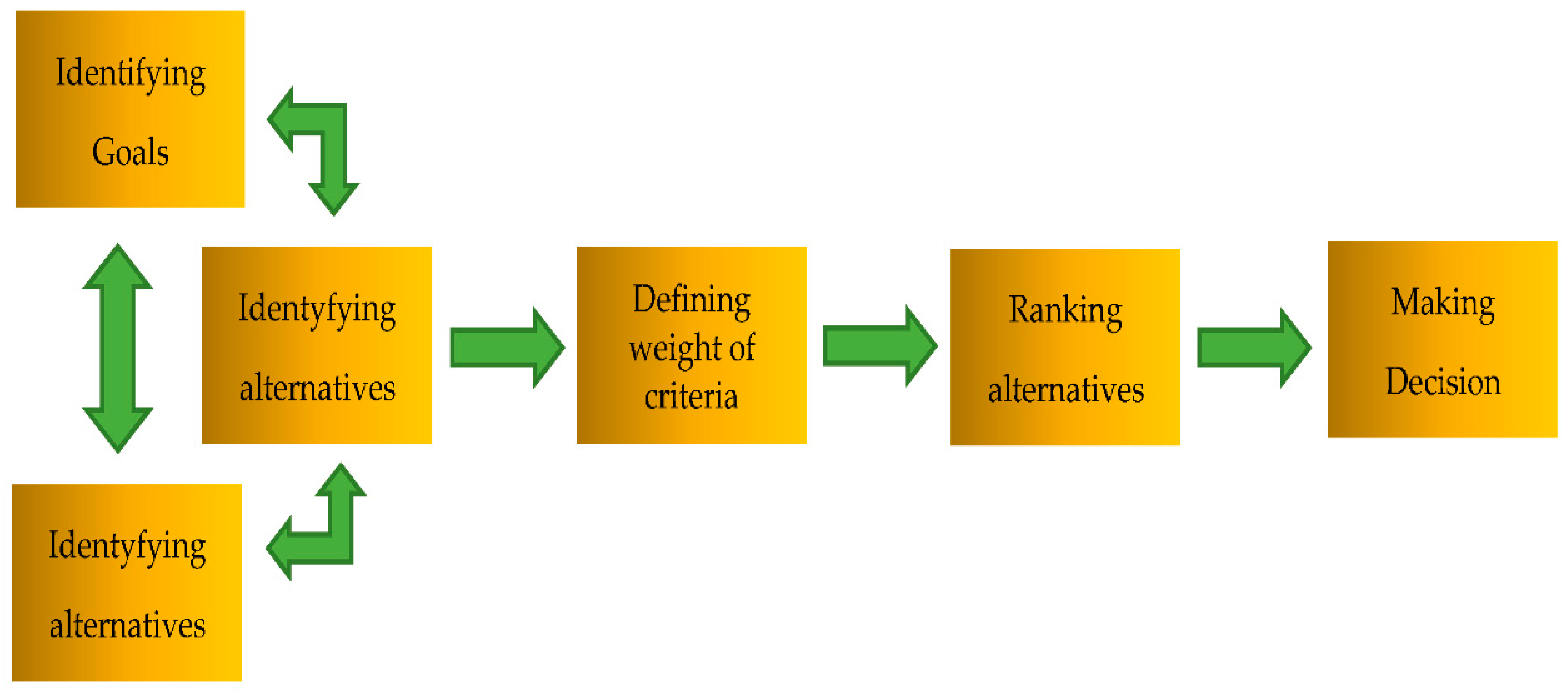
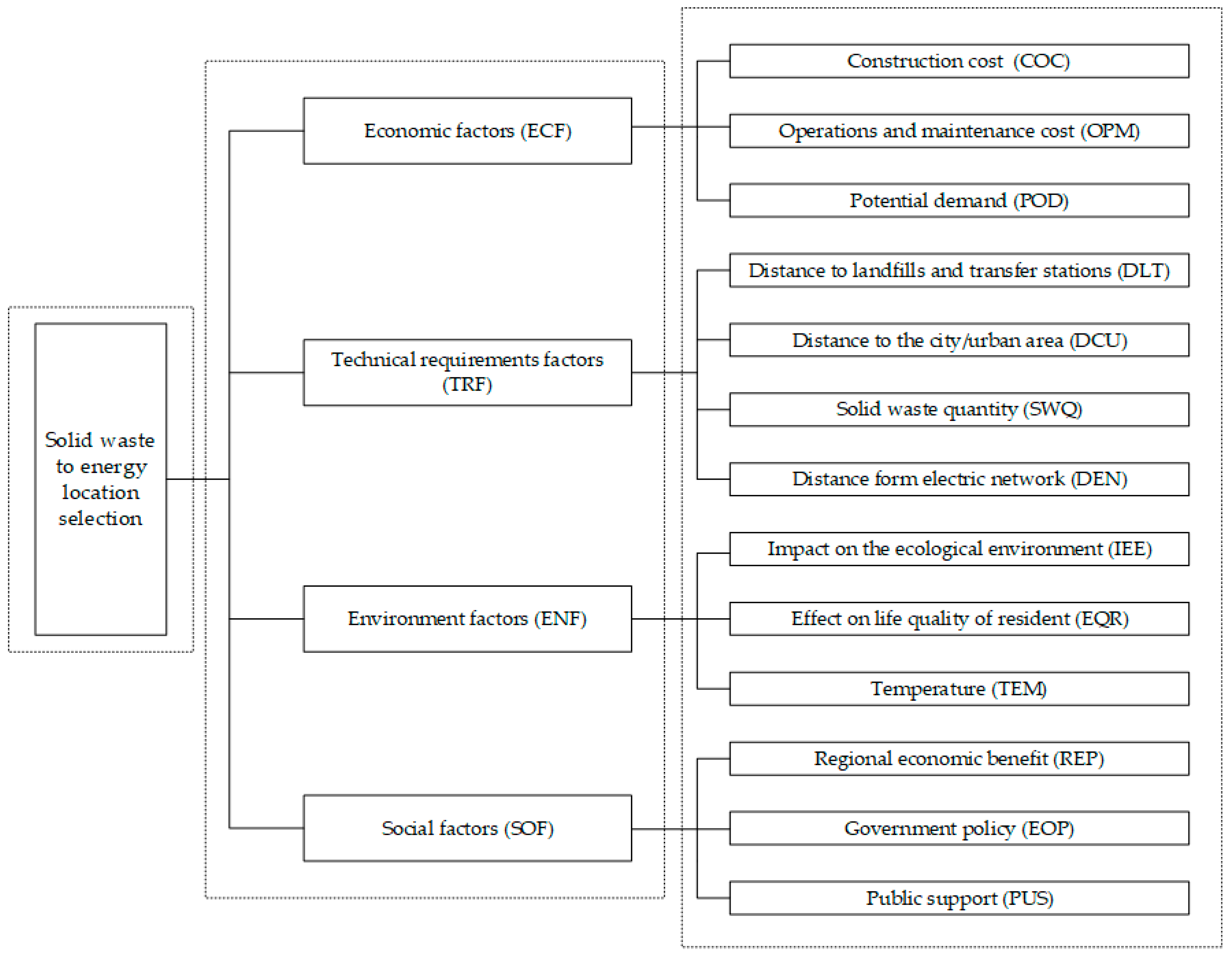
2.1. Research Development
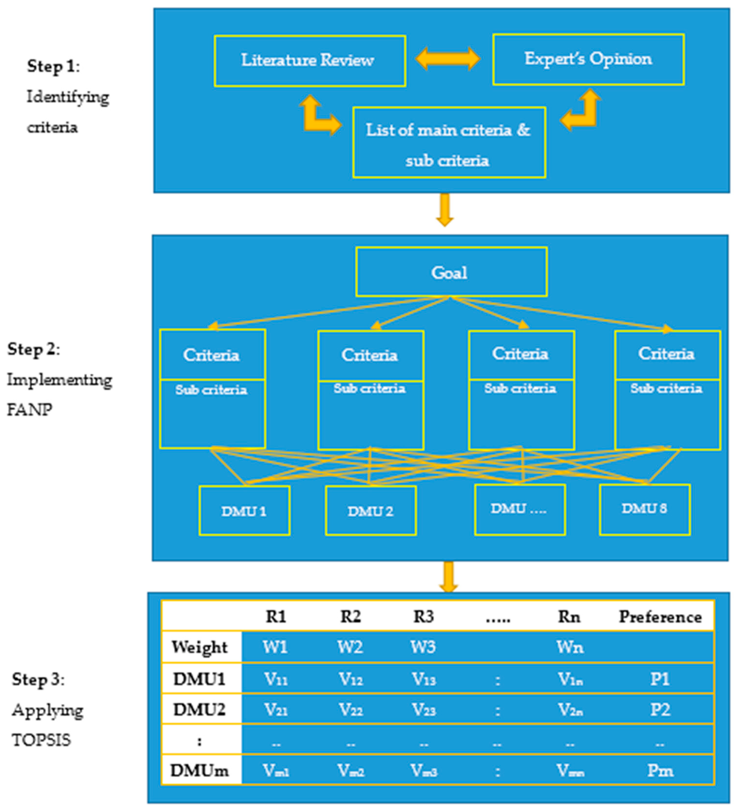
2.2. Methodology
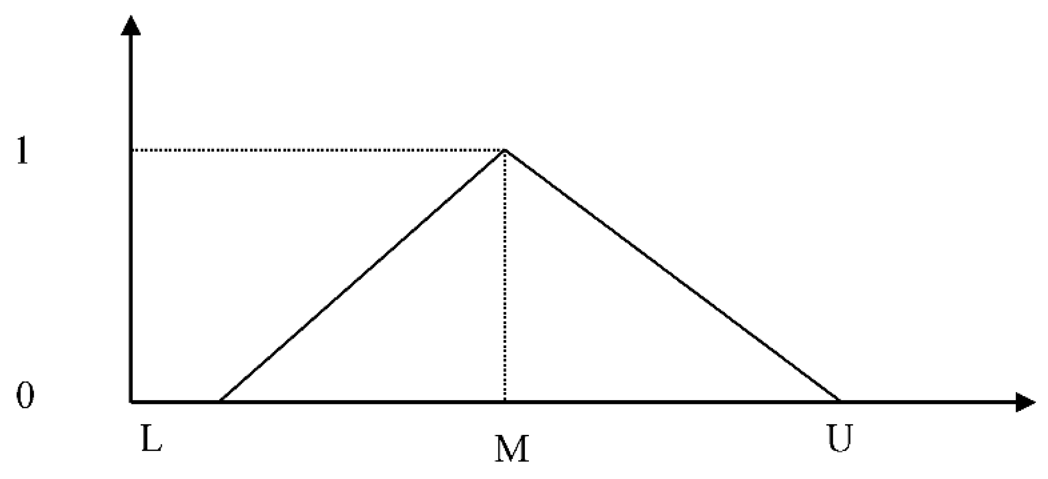
2.2.1. Fuzzy Analytic Network Process (FANP)
- -
- Primary and secondary criteria that control the interactions.
- -
- The grid effect of elements and clusters.
- : the maximum value of the matrix.
- A: Comparative matrix of pairs of elements.
- I: unit matrix of the same level with matrix A.
- CI: consistency index,
- RI: random index.
- is the maximum value of the matrix,
- n is the number of indicators.
- -
- U12 is a matrix formed from the matrix’s own vector when comparing the choices for each criterion.
- -
- U21 is a matrix formed from its own vector when comparing the criteria for each choice.
- -
- U22 is a matrix formed from its own vector when comparing the interaction effect between the criteria.
- -
- U23 is a matrix formed from the matrix’s own vector when comparing the criteria with each other.
2.2.2. TOPSIS Model
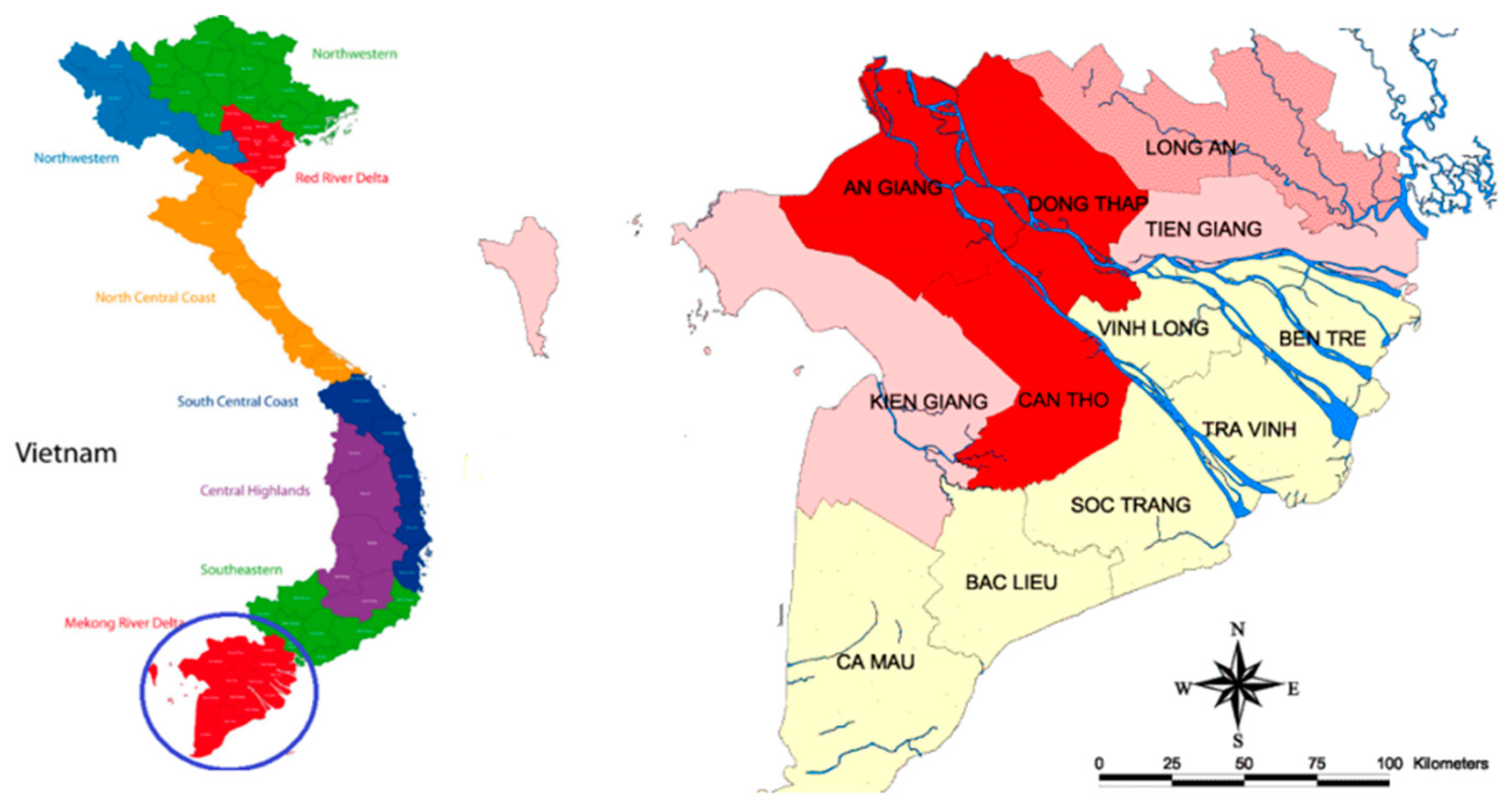
3. Case Study
4. Results and Discussion
5. Conclusions
Author Contributions
Funding
Conflicts of Interest
Appendix A

| Criteria | ENF | SOF | TRF | Weight |
|---|---|---|---|---|
| ENF | (1,1,1) | (3,4,5) | (2,3,4) | 0.625013 |
| SOF | (1/5,1/4,1/3) | (1,1,1) | (1/3,1/2,1) | 0.1365 |
| TRF | (1/4,1/3,1/2) | (1,2,3) | (1,1,1) | 0.238487 |
| Total | 1 | |||
| CR = 0.01759 | ||||
| Criteria | ECF | SOF | TRF | Weight |
|---|---|---|---|---|
| ECF | (1,1,1) | (2,3,4) | (1,2,3) | 0.527836 |
| SOF | (1/4,1/3,1/2) | (1,1,1) | (1/4,1/3,1/2) | 0.139648 |
| TRF | (1/3,1/2,1) | (2,3,4) | (1,1,1) | 0.332516 |
| Total | 1 | |||
| CR = 0.05156 | ||||
| Criteria | ECF | ENF | TRF | Weight |
|---|---|---|---|---|
| ECF | (1,1,1) | (3,4,5) | (1,2,3) | 0.58417 |
| ENF | (1/5,1/4,1/3) | (1,1,1) | (1,1,1) | 0.184002 |
| TRF | (1/3,1/2,1) | (1,1,1) | (1,1,1) | 0.231828 |
| Total | 1 | |||
| CR = 0.05156 | ||||
| Criteria | ECF | ENF | SOF | Weight |
|---|---|---|---|---|
| ECF | (1,1,1) | (2,3,4) | (4,5,6) | 0.636986 |
| ENF | (1/4,1/3,1/2) | (1,1,1) | (2,3,4) | 0.258285 |
| SOF | (1/6,1/5,1/4) | (1/4,1/3,1/2) | (1,1,1) | 0.104729 |
| Total | 1 | |||
| CR = 0.03703 | ||||
| Subcriteria | COC | OPM | POD | Weight |
|---|---|---|---|---|
| COC | (1,1,1) | (2,3,4) | (2,3,4) | 0.593634 |
| OPM | (1/4,1/3,1/2) | (1,1,1) | (1,2,3) | 0.249311 |
| POD | (1/4,1/3,1/2) | (1/3,1/2,1) | (1,1,1) | 0.157056 |
| Total | 1 | |||
| CR = 0.05156 | ||||
| Subcriteria | EQR | IEE | TEM | Weight |
|---|---|---|---|---|
| EQR | (1,1,1) | (2,3,4) | (1,2,3) | 0.549946 |
| IEE | (1/4,1/3,1/2) | (1,1,1) | (1,1,1) | 0.209843 |
| TEM | (1/3,1/2,1) | (1,1,1) | (1,1,1) | 0.240211 |
| Total | 1 | |||
| CR = 0.01759 | ||||
| Subcriteria | EOP | PUS | REP | Weight |
|---|---|---|---|---|
| EOP | (1,1,1) | (1/3,1/2,1) | (2,3,4) | 0.319618 |
| PUS | (1,2,3) | (1,1,1) | (3,4,5) | 0.558425 |
| REP | (1/4,1/3,1/2) | (1/5,1/4,1/3) | (1,1,1) | 0.121957 |
| Total | 1 | |||
| CR = 0.01759 | ||||
| Subcriteria | DCU | DEN | DLT | SWQ | Weight |
|---|---|---|---|---|---|
| DCU | (1,1,1) | (2,3,4) | (1/4,1/3,1/2) | (2,3,4) | 0.280225 |
| DEN | (1/4,1/3,1/2) | (1,1,1) | (1/5,1/4,1/3) | (1/3,1/2,1) | 0.090176 |
| DLT | (2,3,4) | (3,4,5) | (1,1,1) | (1,2,3) | 0.471381 |
| SWQ | (1/4,1/3,1/2) | (1,2,3) | (1/3,1/2,1) | (1,1,1) | 0.158218 |
| Total | 1 | ||||
| CR = 0.08237 | |||||
| Subcriteria | OPM | POD | Weight |
|---|---|---|---|
| OPM | (1,1,1) | (3,4,5) | 0.8 |
| POD | (1/5,1/4,1/3) | (1,1,1) | 0.2 |
| Total | 1 | ||
| CR = 0 | |||
| Subcriteria | DEN | DLT | SWQ | Weight |
|---|---|---|---|---|
| DEN | (1,1,1) | (1,2,3) | (1/3,1/2,1) | 0.296961294 |
| DLT | (1/3,1/2,1) | (1,1,1) | (1/4,1/3,1/2) | 0.163424044 |
| SWQ | (1,2,3) | (2,3,4) | (1,1,1) | 0.539614662 |
| Total | 1 | |||
| CR = 0.00885 | ||||
| Subcriteria | DCU | DLT | SWQ | Weight |
|---|---|---|---|---|
| DCU | (1,1,1) | (3,4,5) | (1,2,3) | 0.558424506 |
| DLT | (1/5,1/4,1/3) | (1,1,1) | (1/4,1/3,1/2) | 0.121957144 |
| SWQ | (1/3,1/2,1) | (2,3,4) | (1,1,1) | 0.319618349 |
| Total | 1 | |||
| CR = 0.01759 | ||||
| Subcriteria | DCU | DEN | SWQ | Weight |
|---|---|---|---|---|
| DCU | (1,1,1) | (1/4,1/3,1/2) | (1,2,3) | 0.249310377 |
| DEN | (2,3,4) | (1,1,1) | (2,3,4) | 0.593633926 |
| SWQ | (1/3,1/2,1) | (1/4,1/3,1/2) | (1,1,1) | 0.157055696 |
| Total | 1 | |||
| CR = 0.05156 | ||||
| Subcriteria | DCU | DEN | DLT | Weight |
|---|---|---|---|---|
| DCU | (1,1,1) | (4,5,6) | (3,4,5) | 0.673810543 |
| DEN | (1/6,1/5,1/4) | (1,1,1) | (1/4,1/3,1/2) | 0.100653892 |
| DLT | (1/5,1/4,1/3) | (2,3,4) | (1,1,1) | 0.225535565 |
| Total | 1 | |||
| CR = 0.08247 | ||||
| Subcriteria | PUS | REP | Weight |
|---|---|---|---|
| PUS | (1,1,1) | (1/6,1/5,1/4) | 0.166667 |
| REP | (4,5,6) | (1,1,1) | 0.833333 |
| Total | 1 | ||
| CR = 0 | |||
| Subcriteria | IEE | TEM | Weight |
|---|---|---|---|
| IEE | (1,1,1) | (4,5,6) | 0.833333 |
| TEM | (1/6,1/5,1/4) | (1,1,1) | 0.166667 |
| Total | 1 | ||
| CR = 0 | |||
| Subcriteria | EQR | TEM | Weight |
|---|---|---|---|
| EQR | (1,1,1) | (5,6,7) | 0.857142857 |
| TEM | (1/7,1/6,1/5) | (1,1,1) | 0.142857143 |
| Total | 1 | ||
| CR = 0 | |||
| Alternatives | COC | POD | Weight |
|---|---|---|---|
| COC | (1,1,1) | (1/6,1/5,1/4) | 0.166666667 |
| POD | (4,5,6) | (1,1,1) | 0.833333333 |
| Total | 1 | ||
| CR = 0 | |||
| Subcriteria | COC | OPM | Weight |
|---|---|---|---|
| COC | (1,1,1) | (3,4,5) | 0.8 |
| OPM | (1/5,1/4,1/3) | (1,1,1) | 0.2 |
| Total | 1 | ||
| CR = 0 | |||
| Subcriteria | EOP | REP | Weight |
|---|---|---|---|
| EOP | (1,1,1) | (2,3,4) | 0.75 |
| REP | (1/4,1/3,1/2) | (1,1,1) | 0.25 |
| Total | 1 | ||
| CR = 0 | |||
| Subcriteria | EOP | PUS | Weight |
|---|---|---|---|
| EOP | (1,1,1) | (1/3,1/2,1) | 0.333333333 |
| PUS | (1,2,3) | (1,1,1) | 0.666666667 |
| Total | 1 | ||
| CR = 0 | |||
| Subcriteria | EQR | IEE | Weight |
|---|---|---|---|
| EQR | (1,1,1) | (1/4,1/3,1/2) | 0.249999813 |
| IEE | (2,3,4) | (1,1,1) | 0.750000187 |
| Total | 1 | ||
| CR = 0 | |||
| DMU 8 | DMU 1 | DMU 2 | DMU 3 | DMU 4 | DMU 5 | DMU 6 | DMU 7 | Weight | |
|---|---|---|---|---|---|---|---|---|---|
| DMU 8 | (1,1,1) | (1,1,1) | (2,3,4) | (1/4,1/3,1/2) | (3,4,5) | (1,2,3) | (2,3,4) | (3,4,5) | 0.1752 |
| DMU 1 | (1,1,1) | (1,1,1) | (2,3,4) | (1/3,1/2,1) | (3,4,5) | (2,3,4) | (5,6,7) | (4,5,6) | 0.2164 |
| DMU 2 | (1/4,1/3,1/2) | (1/4,1/3,1/2) | (1,1,1) | (1/4,1/3,1/2) | (1/4,1/3,1/2) | (1/5,1/4,1/3) | (1/3,1/2,1) | (2,3,4) | 0.0506 |
| DMU 3 | (2,3,4) | (1,2,3) | (2,3,4) | (1,1,1) | (3,4,5) | (1,2,3) | (2,3,4) | (4,5,6) | 0.2617 |
| DMU 4 | (1/5,1/4,1/3) | (1/5,1/4,1/3) | (2,3,4) | (1/5,1/4,1/3) | (1,1,1) | (2,3,4) | (1,2,3) | (3,4,5) | 0.1067 |
| DMU 5 | (1/3,1/2,1) | (1/4,1/3,1/2) | (3,4,5) | (1/3,1/2,1) | (1/4,1/3,1/2) | (1,1,1) | (1,2,3) | (1,2,3) | 0.0914 |
| DMU 6 | (1/4,1/3,1/2) | (1/7,1/6,1/5) | (1,2,3) | (1/4,1/3,1/2) | (1/3,1/2,1) | (1/3,1/2,1) | (1,1,1) | (4,5,6) | 0.0674 |
| DMU 7 | (1/5,1/4,1/3) | (1/6,1/5,1/4) | 1/3 | (1/6,1/5,1/4) | (1/5,1/4,1/3) | (1/3,1/2,1) | (1/6,1/5,1/4) | (1,1,1) | 0.0305 |
| Total | 1 | ||||||||
| CR = 0.09491 | |||||||||
| DMU 8 | DMU 1 | DMU 2 | DMU 3 | DMU 4 | DMU 5 | DMU 6 | DMU 7 | Weight | |
|---|---|---|---|---|---|---|---|---|---|
| DMU 8 | (1,1,1) | (3,4,5) | (1,2,3) | (5,6,7) | (4,5,6) | (2,3,4) | (1,2,3) | (3,4,5) | 0.2947 |
| DMU 1 | (1/5,1/4,1/3) | (1,1,1) | (3,4,5) | (1,2,3) | (4,5,6) | (2,3,4) | (1,1,1) | (2,3,4) | 0.1825 |
| DMU 2 | (1/3,1/2,1) | (1/5,1/4,1/3) | (1,1,1) | (3,4,5) | (1,2,3) | (1,2,3) | (1/5,1/4,1/3) | (1,2,3) | 0.1006 |
| DMU 3 | (1/7,1/6,1/5) | (1/3,1/2,1) | (1/5,1/4,1/3) | (1,1,1) | (1/4,1/3,1/2) | (1/3,1/2,1) | (1/5,1/4,1/3) | (1/3,1/2,1) | 0.0386 |
| DMU 4 | (1/6,1/5,1/4) | (1/6,1/5,1/4) | (1/3,1/2,1) | (2,3,4) | (1,1,1) | (1/4,1/3,1/2) | (1/4,1/3,1/2) | (1/3,1/2,1) | 0.0494 |
| DMU 5 | (1/5,1/4,1/3) | (1/4,1/3,1/2) | (1/3,1/2,1) | (1,2,3) | (2,3,4) | (1,1,1) | (1/5,1/4,1/3) | (1/4,1/3,1/2) | 0.0650 |
| DMU 6 | (1/4,1/3,1/2) | (1,1,1) | (3,4,5) | (3,4,5) | (2,3,4) | (3,4,5) | (1,1,1) | (1,2,3) | 0.1864 |
| DMU 7 | (1/5,1/4,1/3) | (1/4,1/3,1/2) | (1/3,1/2,1) | (1,2,3) | (1,2,3) | (2,3,4) | (1/3,1/2,1) | (1,1,1) | 0.0828 |
| Total | 1 | ||||||||
| CR = 0.08515 | |||||||||
| DMU 8 | DMU 1 | DMU 2 | DMU 3 | DMU 4 | DMU 5 | DMU 6 | DMU 7 | Weight | |
|---|---|---|---|---|---|---|---|---|---|
| DMU 8 | (1,1,1) | (3,4,5) | (2,3,4) | (1,2,3) | (4,5,6) | (3,4,5) | (2,3,4) | (1,2,3) | 0.2948 |
| DMU 1 | (1/5,1/4,1/3) | (1,1,1) | (3,4,5) | (5,6,7) | (4,5,6) | (2,3,4) | (2,3,4) | (1,2,3) | 0.2200 |
| DMU 2 | (1/4,1/3,1/2) | (1/5,1/4,1/3) | (1,1,1) | (3,4,5) | (2,3,4) | (1,2,3) | (2,3,4) | (1/3,1/2,1) | 0.1141 |
| DMU 3 | (1/3,1/2,1) | (1/7,1/6,1/5) | (1/5,1/4,1/3) | (1,1,1) | (1,1,1) | (1/3,1/2,1) | (1/4,1/3,1/2) | (1/5,1/4,1/3) | 0.0446 |
| DMU 4 | (1/6,1/5,1/4) | (1/6,1/5,1/4) | (1/4,1/3,1/2) | (1,1,1) | (1,1,1) | (1/4,1/3,1/2) | (1/4,1/3,1/2) | (1/3,1/2,1) | 0.0392 |
| DMU 5 | (1/5,1/4,1/3) | (1/4,1/3,1/2) | (1/3,1/2,1) | (1,2,3) | (2,3,4) | (1,1,1) | (1,1,1) | (1/4,1/3,1/2) | 0.0687 |
| DMU 6 | (1/4,1/3,1/2) | (1/4,1/3,1/2) | (1/4,1/3,1/2) | (2,3,4) | (2,3,4) | (1,1,1) | (1,1,1) | (1/3,1/2,1) | 0.0771 |
| DMU 7 | (1/3,1/2,1) | (1/3,1/2,1) | (1,2,3) | (3,4,5) | (1,2,3) | (2,3,4) | (1,2,3) | (1,1,1) | 0.1415 |
| Total | 1 | ||||||||
| CR = 0.08044 | |||||||||
| DMU 8 | DMU 1 | DMU 2 | DMU 3 | DMU 4 | DMU 5 | DMU 6 | DMU 7 | Weight | |
|---|---|---|---|---|---|---|---|---|---|
| DMU 8 | (1,1,1) | (1/4,1/3,1/2) | (1/5,1/4,1/3) | (1/4,1/3,1/2) | (1/4,1/3,1/2) | (1/3,1/2,1) | (1/5,1/4,1/3) | (1/4,1/3,1/2) | 0.0398 |
| DMU 1 | (2,3,4) | (1,1,1) | (1/3,1/2,1) | (1/4,1/3,1/2) | (1/5,1/4,1/3) | (1/3,1/2,1) | (1/4,1/3,1/2) | (1/5,1/4,1/3) | 0.0538 |
| DMU 2 | (3,4,5) | (1,2,3) | (1,1,1) | (1/6,1/5,1/4) | (1/3,1/2,1) | (1/4,1/3,1/2) | (1/5,1/4,1/3) | (1/3,1/2,1) | 0.0686 |
| DMU 3 | (2,3,4) | (2,3,4) | (4,5,6) | (1,1,1) | (2,3,4) | (3,4,5) | (1,2,3) | (3,4,5) | 0.2903 |
| DMU 4 | (2,3,4) | (3,4,5) | (1,2,3) | (1/4,1/3,1/2) | (1,1,1) | (1,2,3) | (1,1,1) | (2,3,4) | 0.1620 |
| DMU 5 | (1,2,3) | (1,2,3) | (2,3,4) | (1/5,1/4,1/3) | (1/3,1/2,1) | (1,1,1) | (1/5,1/4,1/3) | (1/4,1/3,1/2) | 0.0806 |
| DMU 6 | (3,4,5) | (2,3,4) | (3,4,5) | (1/3,1/2,1) | (1,1,1) | (3,4,5) | (1,1,1) | (1,2,3) | 0.1862 |
| DMU 7 | (2,3,4) | (3,4,5) | (1,2,3) | (1/5,1/4,1/3) | (1/4,1/3,1/2) | (2,3,4) | (1/3,1/2,1) | (1,1,1) | 0.1188 |
| Total | 1 | ||||||||
| CR = 0.08709 | |||||||||
| DMU 8 | DMU 1 | DMU 2 | DMU 3 | DMU 4 | DMU 5 | DMU 6 | DMU 7 | Weight | |
|---|---|---|---|---|---|---|---|---|---|
| DMU 8 | (1,1,1) | (2,3,4) | (1,2,3) | (1/4,1/3,1/2) | (1/3,1/2,1) | (1,2,3) | (2,3,4) | (3,4,5) | 0.1527 |
| DMU 1 | (1/4,1/3,1/2) | (1,1,1) | (1,2,3) | (1/3,1/2,1) | (1/5,1/4,1/3) | (1/6,1/5,1/4) | (2,3,4) | (1,2,3) | 0.0755 |
| DMU 2 | (1/3,1/2,1) | (1/3,1/2,1) | (1,1,1) | (1/4,1/3,1/2) | (1/6,1/5,1/4) | (1/3,1/2,1) | (1,2,3) | (2,3,4) | 0.0660 |
| DMU 3 | (2,3,4) | (1,2,3) | (2,3,4) | (1,1,1) | (1/5,1/4,1/3) | (1/3,1/2,1) | (2,3,4) | (3,4,5) | 0.1610 |
| DMU 4 | (1,2,3) | (3,4,5) | (4,5,6) | (3,4,5) | (1,1,1) | (1,2,3) | (2,3,4) | (4,5,6) | 0.2891 |
| DMU 5 | (1/3,1/2,1) | (4,5,6) | (1,2,3) | (1,2,3) | (1/3,1/2,1) | (1,1,1) | (2,3,4) | (3,4,5) | 0.1722 |
| DMU 6 | (1/4,1/3,1/2) | (1/4,1/3,1/2) | (1/3,1/2,1) | (1/4,1/3,1/2) | (1/4,1/3,1/2) | (1/4,1/3,1/2) | (1,1,1) | (1,2,3) | 0.0495 |
| DMU 7 | (1/5,1/4,1/3) | (1/3,1/2,1) | (1/4,1/3,1/2) | (1/5,1/4,1/3) | (1/6,1/5,1/4) | (1/5,1/4,1/3) | (1/3,1/2,1) | (1,1,1) | 0.0340 |
| Total | 1 | ||||||||
| CR = 0.07805 | |||||||||
| DMU 8 | DMU 1 | DMU 2 | DMU 3 | DMU 4 | DMU 5 | DMU 6 | DMU 7 | Weight | |
|---|---|---|---|---|---|---|---|---|---|
| DMU 8 | (1,1,1) | (1,2,3) | (3,4,5) | (1,2,3) | (2,3,4) | (1/4,1/3,1/2) | (2,3,4) | (1,2,3) | 0.1888 |
| DMU 1 | (1/3,1/2,1) | (1,1,1) | (3,4,5) | (2,3,4) | (1,2,3) | (1/4,1/3,1/2) | (1/3,1/2,1) | (2,3,4) | 0.1247 |
| DMU 2 | (1/5,1/4,1/3) | (1/5,1/4,1/3) | (1,1,1) | (1/3,1/2,1) | (1/4,1/3,1/2) | (1/5,1/4,1/3) | (1/5,1/4,1/3) | (1/3,1/2,1) | 0.0362 |
| DMU 3 | (1/3,1/2,1) | (1/4,1/3,1/2) | (1,2,3) | (1,1,1) | (1,2,3) | (1/4,1/3,1/2) | (1/5,1/4,1/3) | (1/3,1/2,1) | 0.0683 |
| DMU 4 | (1/4,1/3,1/2) | (1/3,1/2,1) | (2,3,4) | (1/3,1/2,1) | (1,1,1) | (1/4,1/3,1/2) | (1/4,1/3,1/2) | (2,3,4) | 0.0785 |
| DMU 5 | (2,3,4) | (2,3,4) | (3,4,5) | (2,3,4) | (2,3,4) | (1,1,1) | (1,2,3) | (4,5,6) | 0.2793 |
| DMU 6 | (1/4,1/3,1/2) | (1,2,3) | (3,4,5) | (3,4,5) | (2,3,4) | (1/3,1/2,1) | (1,1,1) | (1,2,3) | 0.1591 |
| DMU 7 | (1/3,1/2,1) | (1/4,1/3,1/2) | (1,2,3) | (1,2,3) | (1/4,1/3,1/2) | (1/6,1/5,1/4) | (1/3,1/2,1) | (1,1,1) | 0.0652 |
| Total | 1 | ||||||||
| CR = 0.07845 | |||||||||
| DMU 8 | DMU 1 | DMU 2 | DMU 3 | DMU 4 | DMU 5 | DMU 6 | DMU 7 | Weight | |
|---|---|---|---|---|---|---|---|---|---|
| DMU 8 | (1,1,1) | (1,2,3) | (1,2,3) | (2,3,4) | (1/5,1/4,1/3) | (1,2,3) | (3,4,5) | (1,1,1) | 0.1577 |
| DMU 1 | (1/3,1/2,1) | (1,1,1) | (2,3,4) | (3,4,5) | (1/3,1/2,1) | (3,4,5) | (2,3,4) | (2,3,4) | 0.1843 |
| DMU 2 | (1/3,1/2,1) | (1/4,1/3,1/2) | (1,1,1) | (1/3,1/2,1) | (1/5,1/4,1/3) | (1/3,1/2,1) | (1/3,1/2,1) | (1/5,1/4,1/3) | 0.0437 |
| DMU 3 | (1/4,1/3,1/2) | (1/5,1/4,1/3) | (1,2,3) | (1,1,1) | (1/4,1/3,1/2) | (2,3,4) | (1/3,1/2,1) | (1/4,1/3,1/2) | 0.0685 |
| DMU 4 | (3,4,5) | (1,2,3) | (3,4,5) | (2,3,4) | (1,1,1) | (4,5,6) | (3,4,5) | (2,3,4) | 0.2955 |
| DMU 5 | (1/3,1/2,1) | (1/5,1/4,1/3) | (1,2,3) | (1/4,1/3,1/2) | (1/6,1/5,1/4) | (1,1,1) | (1,2,3) | (1/4,1/3,1/2) | 0.0592 |
| DMU 6 | (1/5,1/4,1/3) | (1/4,1/3,1/2) | (1,2,3) | (1,2,3) | (1/5,1/4,1/3) | (1/3,1/2,1) | (1,1,1) | (1/3,1/2,1) | 0.0630 |
| DMU 7 | (1,1,1) | (1/4,1/3,1/2) | (3,4,5) | (2,3,4) | (1/4,1/3,1/2) | (2,3,4) | (1,2,3) | (1,1,1) | 0.1280 |
| Total | 1 | ||||||||
| CR = 0.0839 | |||||||||
| DMU 8 | DMU 1 | DMU 2 | DMU 3 | DMU 4 | DMU 5 | DMU 6 | DMU 7 | Weight | |
|---|---|---|---|---|---|---|---|---|---|
| DMU 8 | (1,1,1) | (1,2,3) | (3,4,5) | (1,2,3) | (2,3,4) | (2,3,4) | (1,1,1) | (1,2,3) | 0.2218 |
| DMU 1 | (1/3,1/2,1) | (1,1,1) | (3,4,5) | (2,3,4) | (1,2,3) | (4,5,6) | (2,3,4) | (1,2,3) | 0.2114 |
| DMU 2 | (1/5,1/4,1/3) | (1/5,1/4,1/3) | (1,1,1) | (1/4,1/3,1/2) | (1/5,1/4,1/3) | (1/3,1/2,1) | (1/5,1/4,1/3) | (1/4,1/3,1/2) | 0.0350 |
| DMU 3 | (1/3,1/2,1) | (1/4,1/3,1/2) | (2,3,4) | (1,1,1) | (1/4,1/3,1/2) | (3,4,5) | (1/3,1/2,1) | (1/5,1/4,1/3) | 0.0805 |
| DMU 4 | (1/4,1/3,1/2) | (1/3,1/2,1) | (3,4,5) | (2,3,4) | (1,1,1) | (2,3,4) | (1,2,3) | (1,2,3) | 0.1545 |
| DMU 5 | (1/4,1/3,1/2) | (1/6,1/5,1/4) | (1,2,3) | (1/5,1/4,1/3) | (1/4,1/3,1/2) | (1,1,1) | (1,1,1) | (1/5,1/4,1/3) | 0.0507 |
| DMU 6 | (1,1,1) | (1/4,1/3,1/2) | (3,4,5) | (1,2,3) | (1/3,1/2,1) | (1,1,1) | (1,1,1) | (1/3,1/2,1) | 0.1017 |
| DMU 7 | (1/3,1/2,1) | (1/3,1/2,1) | (2,3,4) | (3,4,5) | (1/3,1/2,1) | (3,4,5) | (1,2,3) | (1,1,1) | 0.1445 |
| Total | 1 | ||||||||
| CR = 0.08162 | |||||||||
| DMU 8 | DMU 1 | DMU 2 | DMU 3 | DMU 4 | DMU 5 | DMU 6 | DMU 7 | Weight | |
|---|---|---|---|---|---|---|---|---|---|
| DMU 8 | (1,1,1) | (2,3,4) | (3,4,5) | (1,2,3) | (2,3,4) | (1,2,3) | (1,1,1) | (1/4,1/3,1/2) | 0.1646 |
| DMU 1 | (1/4,1/3,1/2) | (1,1,1) | (1/3,1/2,1) | (1/5,1/4,1/3) | (1/3,1/2,1) | (1/4,1/3,1/2) | (1/6,1/5,1/4) | (1/5,1/4,1/3) | 0.0368 |
| DMU 2 | (1/5,1/4,1/3) | (1,2,3) | (1,1,1) | (1/3,1/2,1) | (1/5,1/4,1/3) | (1/4,1/3,1/2) | (1/6,1/5,1/4) | (1/5,1/4,1/3) | 0.0410 |
| DMU 3 | (1/3,1/2,1) | (3,4,5) | (1,2,3) | (1,1,1) | (1/3,1/2,1) | (1/4,1/3,1/2) | (1/5,1/4,1/3) | (1/3,1/2,1) | 0.0729 |
| DMU 4 | (1/4,1/3,1/2) | (1,2,3) | (3,4,5) | (1,2,3) | (1,1,1) | (1/4,1/3,1/2) | (1,1,1) | (1/5,1/4,1/3) | 0.0985 |
| DMU 5 | (1/3,1/2,1) | (2,3,4) | (2,3,4) | (2,3,4) | (2,3,4) | (1,1,1) | (1/3,1/2,1) | (1/3,1/2,1) | 0.1344 |
| DMU 6 | (1,1,1) | (4,5,6) | (4,5,6) | (3,4,5) | (1,1,1) | (1,2,3) | (1,1,1) | (2,3,4) | 0.2366 |
| DMU 7 | (2,3,4) | (3,4,5) | (3,4,5) | (1,2,3) | (3,4,5) | (1,2,3) | (1/4,1/3,1/2) | (1,1,1) | 0.2154 |
| Total | 1 | ||||||||
| CR = 0.08708 | |||||||||
| Alternatives | DMU 8 | DMU 1 | DMU 2 | DMU 3 | DMU 4 | DMU 5 | DMU 6 | DMU 7 | Weight |
|---|---|---|---|---|---|---|---|---|---|
| DMU 8 | (1,1,1) | (1,2,3) | (1/3,1/2,1) | (2,3,4) | (1/3,1/2,1) | (1/4,1/3,1/2) | (1,2,3) | (1,1,1) | 0.0980 |
| DMU 1 | (1/3,1/2,1) | (1,1,1) | (1/4,1/3,1/2) | (1,2,3) | (1/5,1/4,1/3) | (1/4,1/3,1/2) | (3,4,5) | (1/5,1/4,1/3) | 0.0726 |
| DMU 2 | (1,2,3) | (2,3,4) | (1,1,1) | (3,4,5) | (1,2,3) | (2,3,4) | (3,4,5) | (1,2,3) | 0.2451 |
| DMU 3 | (1/4,1/3,1/2) | (1/3,1/2,1) | (1/5,1/4,1/3) | (1,1,1) | (1/6,1/5,1/4) | (1/3,1/2,1) | (1/4,1/3,1/2) | (1/5,1/4,1/3) | 0.0381 |
| DMU 4 | (1,2,3) | (3,4,5) | (1/3,1/2,1) | (4,5,6) | (1,1,1) | (1,2,3) | (2,3,4) | (3,4,5) | 0.2202 |
| DMU 5 | (2,3,4) | (2,3,4) | (1/4,1/3,1/2) | (1,2,3) | (1/3,1/2,1) | (1,1,1) | (1,2,3) | (2,3,4) | 0.1564 |
| DMU 6 | (1/3,1/2,1) | (1/5,1/4,1/3) | (1/5,1/4,1/3) | (2,3,4) | (1/4,1/3,1/2) | (1/3,1/2,1) | (1,1,1) | (1/3,1/2,1) | 0.0572 |
| DMU 7 | (1,1,1) | (3,4,5) | (1/3,1/2,1) | (3,4,5) | (1/5,1/4,1/3) | (1/4,1/3,1/2) | (1,2,3) | (1,1,1) | 0.1124 |
| Total | 1 | ||||||||
| CR = 0.08884 | |||||||||
| Alternatives | DMU 8 | DMU 1 | DMU 2 | DMU 3 | DMU 4 | DMU 5 | DMU 6 | DMU 7 | Weight |
|---|---|---|---|---|---|---|---|---|---|
| DMU 8 | (1,1,1) | (2,3,4) | (3,4,5) | (1,2,3) | (2,3,4) | (2,3,4) | (1,1,1) | (2,3,4) | 0.2425 |
| DMU 1 | (1/4,1/3,1/2) | (1,1,1) | (4,5,6) | (1,2,3) | (2,3,4) | (3,4,5) | (1,2,3) | (5,6,7) | 0.2306 |
| DMU 2 | (1/5,1/4,1/3) | (1/6,1/5,1/4) | (1,1,1) | (1/5,1/4,1/3) | (1/3,1/2,1) | (1/4,1/3,1/2) | (1/4,1/3,1/2) | (1/3,1/2,1) | 0.0361 |
| DMU 3 | (1/3,1/2,1) | (1/3,1/2,1) | (3,4,5) | (1,1,1) | (2,3,4) | (3,4,5) | (1,2,3) | (1,1,1) | 0.1478 |
| DMU 4 | (1/4,1/3,1/2) | (1/4,1/3,1/2) | (1,2,3) | (1/4,1/3,1/2) | (1,1,1) | (1/4,1/3,1/2) | (1/3,1/2,1) | (1/5,1/4,1/3) | 0.0500 |
| DMU 5 | (1/4,1/3,1/2) | (1/5,1/4,1/3) | (2,3,4) | (1/5,1/4,1/3) | (2,3,4) | (1,1,1) | (1/4,1/3,1/2) | (1/3,1/2,1) | 0.0670 |
| DMU 6 | (1,1,1) | (1/3,1/2,1) | (2,3,4) | (1/3,1/2,1) | (1,2,3) | (2,3,4) | (1,1,1) | (1,2,3) | 0.1316 |
| DMU 7 | (1/4,1/3,1/2) | (1/7,1/6,1/5) | (1,2,3) | (1,1,1) | (3,4,5) | (1,2,3) | (1/3,1/2,1) | (1,1,1) | 0.0944 |
| Total | 1 | ||||||||
| CR = 0.08413 | |||||||||
| DMU 8 | DMU 1 | DMU 2 | DMU 3 | DMU 4 | DMU 5 | DMU 6 | DMU 7 | Weight | |
|---|---|---|---|---|---|---|---|---|---|
| DMU 8 | (1,1,1) | (1/3,1/2,1) | (1/5,1/4,1/3) | (1/4,1/3,1/2) | (1/4,1/3,1/2) | (1/5,1/4,1/3) | (1/3,1/2,1) | (1/4,1/3,1/2) | 0.0404 |
| DMU 1 | (1,2,3) | (1,1,1) | (1/7,1/6,1/5) | (1/5,1/4,1/3) | (1/4,1/3,1/2) | (1/3,1/2,1) | (1/5,1/4,1/3) | (1/3,1/2,1) | 0.0446 |
| DMU 2 | (3,4,5) | (5,6,7) | (1,1,1) | (1,1,1) | (1,2,3) | (3,4,5) | (2,3,4) | (4,5,6) | 0.2613 |
| DMU 3 | (2,3,4) | (3,4,5) | (1,1,1) | (1,1,1) | (1,2,3) | (1,2,3) | (3,4,5) | (2,3,4) | 0.2183 |
| DMU 4 | (2,3,4) | (2,3,4) | (1/3,1/2,1) | (1/3,1/2,1) | (1,1,1) | (2,3,4) | (1,2,3) | (3,4,5) | 0.1639 |
| DMU 5 | (3,4,5) | (1,2,3) | (1/5,1/4,1/3) | (1/3,1/2,1) | (1/4,1/3,1/2) | (1,1,1) | (1,2,3) | (3,4,5) | 0.1167 |
| DMU 6 | (1,2,3) | (3,4,5) | (1/4,1/3,1/2) | (1/5,1/4,1/3) | (1/3,1/2,1) | (1/3,1/2,1) | (1,1,1) | (3,4,5) | 0.0990 |
| DMU 7 | (2,3,4) | (1,2,3) | (1/6,1/5,1/4) | (1/4,1/3,1/2) | (1/5,1/4,1/3) | (1/5,1/4,1/3) | (1/5,1/4,1/3) | (1,1,1) | 0.0557 |
| Total | 1 | ||||||||
| CR = 0.07371 | |||||||||
| Alternatives | DMU 8 | DMU 1 | DMU 2 | DMU 3 | DMU 4 | DMU 5 | DMU 6 | DMU 7 | Weight |
|---|---|---|---|---|---|---|---|---|---|
| DMU 8 | (1,1,1) | (1,2,3) | (3,4,5) | (2,3,4) | (4,5,6) | (1/4,1/3,1/2) | (1/4,1/3,1/2) | (1,2,3) | 0.1594 |
| DMU 1 | (1/3,1/2,1) | (1,1,1) | (3,4,5) | (1,2,3) | (3,4,5) | (1/3,1/2,1) | (1,1,1) | (2,3,4) | 0.1488 |
| DMU 2 | (1/5,1/4,1/3) | (1/5,1/4,1/3) | (1,1,1) | (1/4,1/3,1/2) | (1/3,1/2,1) | (1/5,1/4,1/3) | (1/6,1/5,1/4) | (1/3,1/2,1) | 0.0346 |
| DMU 3 | (1/4,1/3,1/2) | (1/3,1/2,1) | (2,3,4) | (1,1,1) | (1/4,1/3,1/2) | (1/5,1/4,1/3) | (1/3,1/2,1) | (1/4,1/3,1/2) | 0.0565 |
| DMU 4 | (1/6,1/5,1/4) | (1/5,1/4,1/3) | (1,2,3) | (2,3,4) | (1,1,1) | (1/3,1/2,1) | (1/4,1/3,1/2) | (1/3,1/2,1) | 0.0684 |
| DMU 5 | (2,3,4) | (1,2,3) | (3,4,5) | (3,4,5) | (1,2,3) | (1,1,1) | (1,2,3) | (2,3,4) | 0.2449 |
| DMU 6 | (2,3,4) | (1,1,1) | (4,5,6) | (1,2,3) | (2,3,4) | (1/3,1/2,1) | (1,1,1) | (4,5,6) | 0.2078 |
| DMU 7 | (1/3,1/2,1) | (1/4,1/3,1/2) | (1,2,3) | (2,3,4) | (1,2,3) | (1/4,1/3,1/2) | (1/6,1/5,1/4) | (1,1,1) | 0.0796 |
| Total | 1 | ||||||||
| CR = 0.0905 | |||||||||
References
- Hou, H.; Li, S.; Lu, Q. Gaseous emission of monocombustion of sewage sludge in a circulating fluidized bed. Ind. Eng. Chem. Res. 2013, 52, 5556–5562. [Google Scholar] [CrossRef]
- United States Environmental Protection Agency. Criteria for the Definition of Solid Waste and Solid and Hazardous Waste Exclusions; EPA: Washington, DC, USA, 2018.
- Costi, P.; Minciardi, R.; Robba, M.; Rovatti, M.; Sacile, R. An environmentally sustainable decision model for urban solid waste management. Waste Manag. 2004, 24, 277–295. [Google Scholar] [CrossRef]
- Fiorucci, P.; Minciardi, R.; Robba, M.; Sacile, R. Solid waste management in urban areas: Development and application of a decision support system. Resour. Conserv. Recycl. 2003, 37, 301–328. [Google Scholar] [CrossRef]
- Nakhla, D.A.; Hassan, M.G.; Haggar, S.E. Impact of biomass in egypt on climate change. Nat. Sci. 2013, 5, 678–684. [Google Scholar] [CrossRef]
- Cheung, W.H.; Lee, V.K.C.; McKay, G. Minimizing dioxin emissions from integrated msw thermal treatment. Environ. Sci. Technol. 2007, 41, 2001–2007. [Google Scholar] [CrossRef] [PubMed]
- Lancia, A.; Karatza, D.; Musmarra, D.; Pepe, F. Adsorption of mercuric chloride from simulated incinerator exhaust gas by means of sorbalittm particles. J. Chem. Eng. Jpn. 1996, 29, 939–946. [Google Scholar] [CrossRef]
- Weinstein, P.E. Waste-to-Energy as a Key Component of Integrated Solid Waste Management for Santiago, Chile: A Cost-Benefit Analysis; Fu Foundation School of Engineering and Applied Science, Columbia University: New York, NY, USA, 2006. [Google Scholar]
- Psomopoulos, C.; Bourka, A.; Themelis, N.J. Waste-to-energy: A review of the status and benefits in USA. Waste Manag. 2009, 29, 1718–1724. [Google Scholar] [CrossRef] [PubMed]
- Hassaan, M.A. A gis-based suitability analysis for siting a solid waste incineration power plant in an urban area case study: Alexandria governorate, Egypt. J. Geogr. Inform. Syst. 2015, 7, 643–657. [Google Scholar] [CrossRef]
- Tavares, G.; Zsigraiová, Z.; Semiao, V. Multi-criteria gis-based siting of an incineration plant for municipal solid waste. Waste Manag. 2011, 31, 1960–1972. [Google Scholar] [CrossRef] [PubMed]
- Yap, H.Y.; Nixon, J.D. A multi-criteria analysis of options for energy recovery from municipal solid waste in India and the UK. Waste Manag. 2015, 46, 265–277. [Google Scholar] [CrossRef] [PubMed] [Green Version]
- Lee, A.H.I.; Kang, H.-Y.; Lin, C.-Y.; Shen, K.-C. An integrated decision-making model for the location of a pv solar plant. Sustainability 2015, 7, 13522–13541. [Google Scholar] [CrossRef]
- Wang, C.-N.; Nguyen, V.T.; Thai, H.T.N.; Duong, D.H. Multi-criteria decision making (MCDM) approaches for solar power plant location selection in viet nam. Energies 2018, 11, 1504. [Google Scholar] [CrossRef]
- Aragonés-Beltrán, P.; Chaparro-González, F.; Ferrando, J.P.P.; García-Melón, M. Selection of photovoltaic solar power plant investment projects-an anp approach. Int. J. Environ. Chem. Ecol. Geol. Geophys. Eng. 2008, 128–136. [Google Scholar] [CrossRef]
- Ali, S.; Lee, S.-M.; Jang, C.-M. Determination of the most optimal on-shore wind farm site location using a GIS-MCDM methodology: Evaluating the case of south korea. Energies 2017, 10, 2072. [Google Scholar] [CrossRef]
- Suh, J.; Brownson, J.R.S. Solar farm suitability using geographic information system fuzzy sets and analytic hierarchy processes: Case study of ulleung island, Korea. Energies 2016, 9, 648. [Google Scholar] [CrossRef]
- Noorollahi, E.; Fadai, D.; Shirazi, M.A.; Ghodsipour, S.H. Land suitability analysis for solar farms exploitation using gis and fuzzy analytic hierarchy process (FAHP)—A case study of Iran. Energies 2016, 9, 643. [Google Scholar] [CrossRef]
- ˇCereška, A.; Zavadskas, E.K.; Bucinskas, V.; Podvezko, V.; Sutinys, E. Analysis of steel wire rope diagnostic data applying multi-criteria methods. Appl. Sci. 2018, 8, 260. [Google Scholar] [CrossRef]
- Reid, R.D.; Sanders, N.R. Operations Management; Wiley: Hoboken, NJ, USA, 2009. [Google Scholar]
- Belton, V.; Stewart, T. Multiple Criteria Decision Analysis: An Integrated Approach; Kluwer Academic: Boston, MA, USA, 2002. [Google Scholar]
- Gan, L.; Xu, D.; Hu, L.; Wang, L. Economic feasibility analysis for renewable energy project using an integrated TFN–AHP–DEA approach on the basis of consumer utility. Energies 2017, 10, 2089. [Google Scholar] [CrossRef]
- Liu, J.-P.; Yang, Q.-R.; He, L. Total-factor energy efficiency (TFEE) evaluation on thermal power industry with DEA, malmquist and multiple regression techniques. Energies 2017, 10, 1039. [Google Scholar] [CrossRef]
- Asadzadeh, A.; Sikder, S.K.; Mahmoudi, F.; Kötter, T. Assessing site selection of new towns using topsis method under entropy logic: A case study: New towns of tehran metropolitan region (TMR). Environ. Manag. Sustain. Dev. 2014, 3, 123–137. [Google Scholar] [CrossRef]
- Rashidi, M.; Ghodrat, M.; Samali, B.; Kendall, B.; Zhang, C. Remedial modelling of steel bridges through application of analytical hierarchy process (AHP). Appl. Sci. 2017, 7, 168. [Google Scholar] [CrossRef]
- Feng, C.-M.; Wang, R.-T. Performance evaluation for airlines including the consideration of financial ratios. J. Air. Transp. Manag. 2000, 6, 133–142. [Google Scholar] [CrossRef]
- Sen, P.; Yang, J.-B. Multiple Criteria Decision Support in Engineering Design; Springer: London, UK, 1998. [Google Scholar]
- Sarkis, J. A strategic decision framework for green supply chain management. J. Clean. Prod. 2003, 11, 397–409. [Google Scholar] [CrossRef]
- Saaty, T.L. Decision Making with Dependence and Feedback: The Analytic Network Process; Rws Publications: Pittsburgh, PA, USA, 1996. [Google Scholar]
- Zadeh, L.A. Fuzzy sets. Inform. Control. 1965, 8, 338–353. [Google Scholar] [CrossRef] [Green Version]
- Lee, A.H.I. A fuzzy supplier selection model with the consideration of benefits, opportunities, costs and risks. Expert. Syst. Appl. 2009, 36, 2879–2893. [Google Scholar] [CrossRef]
- Lee, A.H.I.; Kang, H.-Y.; Hsu, C.-F.; Hung, H.-C. A green supplier selection model for high-tech industry. Expert. Syst. Appl. 2009, 36, 7917–7927. [Google Scholar] [CrossRef]
- Lee, A.H.I.; Kang, H.-Y.; Chang, C.-T. Fuzzy multiple goal programming applied to tft-lcd supplier selection by downstream manufacturers. Expert. Syst. Appl. 2009, 36, 6318–6325. [Google Scholar] [CrossRef]
- Lee, A.H.I.; Kang, H.-Y.; Wang, W.-P. Analysis of priority mix planning for the fabrication of semiconductors under uncertainty. Int. J. Adv. Manuf. Technol. 2006, 28, 351–361. [Google Scholar] [CrossRef]
- Cheng, C.-H. Evaluating weapon systems using ranking fuzzy numbers. Fuzzy Sets Syst. 1999, 107, 25–35. [Google Scholar] [CrossRef]
- Dehghani, M.; Esmaeilian, M.; Tavakkoli-Moghaddam, R. Employing fuzzy anp for green supplier selection and order allocations: A case study. Int. J. Econ. Manag. Soc. Sci. 2013, 2, 565–575. [Google Scholar]
- Kahraman, C.; Ertay, T.; Büyüközkan, G. A fuzzy optimization model for QFD planning process using analytic network approach. Eur. J. Oper. Res. 2006, 171, 390–411. [Google Scholar] [CrossRef] [Green Version]
- Lin, R.; Lin, J.S.-J.; Chang, J.; Tang, D.; Chao, H.; Julian, P.C. Note on group consistency in Analytic Hierarchy Process. Eur. J. Oper. Res. 2008, 190, 672–678. [Google Scholar] [CrossRef]
- Kuswandari, R. Assessment of Different Methods for Measuring the Sustainability of Forest Management Retno Kuswandari; University of Twente: Enschede, The Netherlands, 2004. [Google Scholar]
- Saaty, T.L. The Analytic Hierarchy Process: Planning, Priority Setting, Resources Allocation; McGraw-Hill: New York, NY, USA, 1980. [Google Scholar]
- Hwang, C.-L.; Yoon, K. Multiple Attribute Decision Making: Methods and Applications a State-of-the-Art Survey; Springer: Berlin/Heidelberg, Germany, 1981. [Google Scholar]
- Assari, A.; Maheshand, T.M.; Assari, E. Role of public participation in sustainability of historical city: Usage of topsis method. Indian J. Sci. Technol. 2012, 5, 2289–2294. [Google Scholar]
- Jahanshahloo, G.R.; Lotfi, F.H.; Izadikhah, M. Extension of the topsis method for decision-making problems with fuzzy data. Appl. Math. Comput. 2006, 181, 1544–1551. [Google Scholar] [CrossRef]


| Intensity of Fuzzy Scale | Linguistic Variables for Relative Weights of Criteria |
|---|---|
| Equally important | |
| Moderately important | |
| Strongly important | |
| Very strongly important | |
| Extremely strongly important | |
| Intermediate values between two adjacent judgments; ; ; ; ; |
| Priority Level | Number |
|---|---|
| Equally preferred | 1 |
| Moderately preferred | 3 |
| Strongly preferred | 5 |
| Very strongly preferred | 7 |
| Extremely preferred | 9 |
| Intermediate judgment values | 2, 4, 6, 8 |
| N | 1 | 2 | 3 | 4 | 5 | 6 | 7 | 8 | 9 | 10 |
|---|---|---|---|---|---|---|---|---|---|---|
| R | 0 | 0 | 0.52 | 0.90 | 1.12 | 1.24 | 1.32 | 1.41 | 1.45 | 1.49 |
| 0 | U12 | 0 |
|---|---|---|
| U21 | U22 | U23 |
| 0 | 0 | 0 |
| No | Potential Location | Decision Making Unit (DMU) |
|---|---|---|
| 1 | Long An | DMU 1 |
| 2 | Tien Giang | DMU 2 |
| 3 | Can Tho | DMU 3 |
| 4 | Ben Tre | DMU 4 |
| 5 | An Giang | DMU 5 |
| 6 | Vinh Long | DMU 6 |
| 7 | Dong Thap | DMU 7 |
| 8 | Hau Giang | DMU 8 |
| Criteria | EFC | ENF | SOF | TRF |
|---|---|---|---|---|
| ECF | (1,1,1) | (2,3,4) | (1,2,3) | (3,4,5) |
| ENF | (1/4,1/3,1/2) | (1,1,1) | (1/4,1/3,1/2) | (1,1,1) |
| SOF | (1/3,1/2,1) | (2,3,4) | (1,1,1) | (4,5,6) |
| TRF | (1/5,1/4,1/3) | (1,1,1) | (1/6,1/5,1/4) | (1,1,1) |
| Criteria | ECF | ENF | SOF | TRF |
|---|---|---|---|---|
| ECF | 1 | 3 | 2 | 4 |
| ENF | 1/3 | 1 | 1/3 | 1 |
| SOF | 1/2 | 3 | 1 | 5 |
| TRF | 1/4 | 1 | 1/5 | 1 |
| Criteria | ECF | ENF | SOF | TRF | Weight |
|---|---|---|---|---|---|
| ECF | (1,1,1) | (2,3,4) | (1,2,3) | (3,4,5) | 0.45 |
| ENF | (1/4,1/3,1/2) | (1,1,1) | (1/4,1/3,1/2) | (1,1,1) | 0.12 |
| SOF | (1/3,1/2,1) | (2,3,4) | (1,1,1) | (4,5,6) | 0.33 |
| TRF | (1/5,1/4,1/3) | (1,1,1) | (1/6,1/5,1/4) | (1,1,1) | 0.1 |
| Total | 1 | ||||
| CR = 0.044 | |||||
| No | Subcriteria | Weight |
|---|---|---|
| 1 | COC | 0.09995 |
| 2 | DCU | 0.07521 |
| 3 | DEN | 0.0473 |
| 4 | DLT | 0.03181 |
| 5 | EOP | 0.03948 |
| 6 | EQR | 0.15249 |
| 7 | IEE | 0.16369 |
| 8 | OPM | 0.10082 |
| 9 | POD | 0.10397 |
| 10 | PUS | 0.03423 |
| 11 | REP | 0.04143 |
| 12 | SWQ | 0.06067 |
| 13 | TEM | 0.04896 |
| Subcriteria | DMUs | |||||||
|---|---|---|---|---|---|---|---|---|
| DMU 1 | DMU 2 | DMU 3 | DMU 4 | DMU 5 | DMU 6 | DMU 7 | DMU 8 | |
| COC | 0.0260 | 0.0390 | 0.0520 | 0.0260 | 0.0390 | 0.0260 | 0.0390 | 0.0260 |
| OPM | 0.0472 | 0.0236 | 0.0236 | 0.0472 | 0.0472 | 0.0354 | 0.0236 | 0.0236 |
| POD | 0.0466 | 0.0362 | 0.0310 | 0.0414 | 0.0259 | 0.0414 | 0.0310 | 0.0362 |
| DLT | 0.0106 | 0.0106 | 0.0106 | 0.0106 | 0.0141 | 0.0071 | 0.0106 | 0.0141 |
| DCU | 0.0272 | 0.0272 | 0.0272 | 0.0272 | 0.0272 | 0.0362 | 0.0181 | 0.0181 |
| SWQ | 0.0182 | 0.0243 | 0.0213 | 0.0243 | 0.0243 | 0.0182 | 0.0213 | 0.0182 |
| DEN | 0.0168 | 0.0168 | 0.0112 | 0.0225 | 0.0112 | 0.0225 | 0.0112 | 0.0168 |
| IEE | 0.0452 | 0.0226 | 0.0339 | 0.0565 | 0.0565 | 0.0565 | 0.0565 | 0.1017 |
| EQR | 0.0490 | 0.0490 | 0.0490 | 0.0588 | 0.0294 | 0.0392 | 0.0490 | 0.0882 |
| TEM | 0.0183 | 0.0138 | 0.0183 | 0.0160 | 0.0206 | 0.0160 | 0.0160 | 0.0183 |
| REP | 0.0174 | 0.0116 | 0.0135 | 0.0155 | 0.0155 | 0.0135 | 0.0174 | 0.0116 |
| EOP | 0.0168 | 0.0168 | 0.0131 | 0.0150 | 0.0112 | 0.0131 | 0.0131 | 0.0112 |
| PUS | 0.0124 | 0.0124 | 0.0108 | 0.0093 | 0.0139 | 0.0139 | 0.0124 | 0.0108 |
© 2018 by the authors. Licensee MDPI, Basel, Switzerland. This article is an open access article distributed under the terms and conditions of the Creative Commons Attribution (CC BY) license (http://creativecommons.org/licenses/by/4.0/).
Share and Cite
Wang, C.-N.; Nguyen, V.T.; Duong, D.H.; Thai, H.T.N. A Hybrid Fuzzy Analysis Network Process (FANP) and the Technique for Order of Preference by Similarity to Ideal Solution (TOPSIS) Approaches for Solid Waste to Energy Plant Location Selection in Vietnam. Appl. Sci. 2018, 8, 1100. https://doi.org/10.3390/app8071100
Wang C-N, Nguyen VT, Duong DH, Thai HTN. A Hybrid Fuzzy Analysis Network Process (FANP) and the Technique for Order of Preference by Similarity to Ideal Solution (TOPSIS) Approaches for Solid Waste to Energy Plant Location Selection in Vietnam. Applied Sciences. 2018; 8(7):1100. https://doi.org/10.3390/app8071100
Chicago/Turabian StyleWang, Chia-Nan, Van Thanh Nguyen, Duy Hung Duong, and Hoang Tuyet Nhi Thai. 2018. "A Hybrid Fuzzy Analysis Network Process (FANP) and the Technique for Order of Preference by Similarity to Ideal Solution (TOPSIS) Approaches for Solid Waste to Energy Plant Location Selection in Vietnam" Applied Sciences 8, no. 7: 1100. https://doi.org/10.3390/app8071100