Three-Dimensional Magnetohydrodynamic Mixed Convection Flow of Nanofluids over a Nonlinearly Permeable Stretching/Shrinking Sheet with Velocity and Thermal Slip

Abstract
:
1. Introduction
2. Problem Formulation
3. Stability Analysis
4. Results and Discussion
5. Conclusions
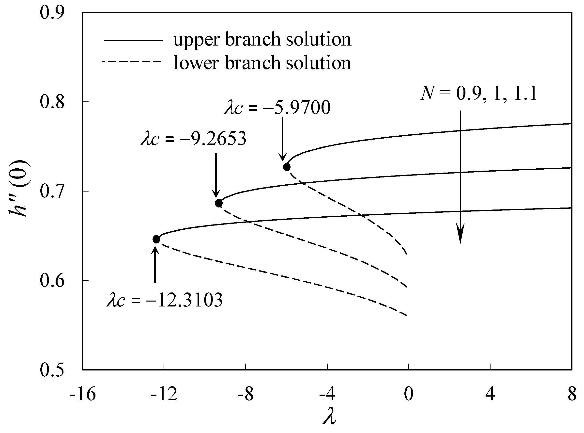
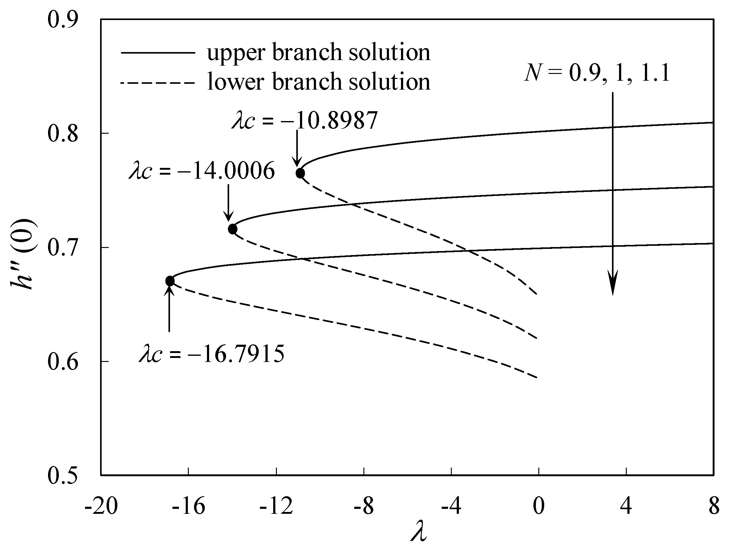
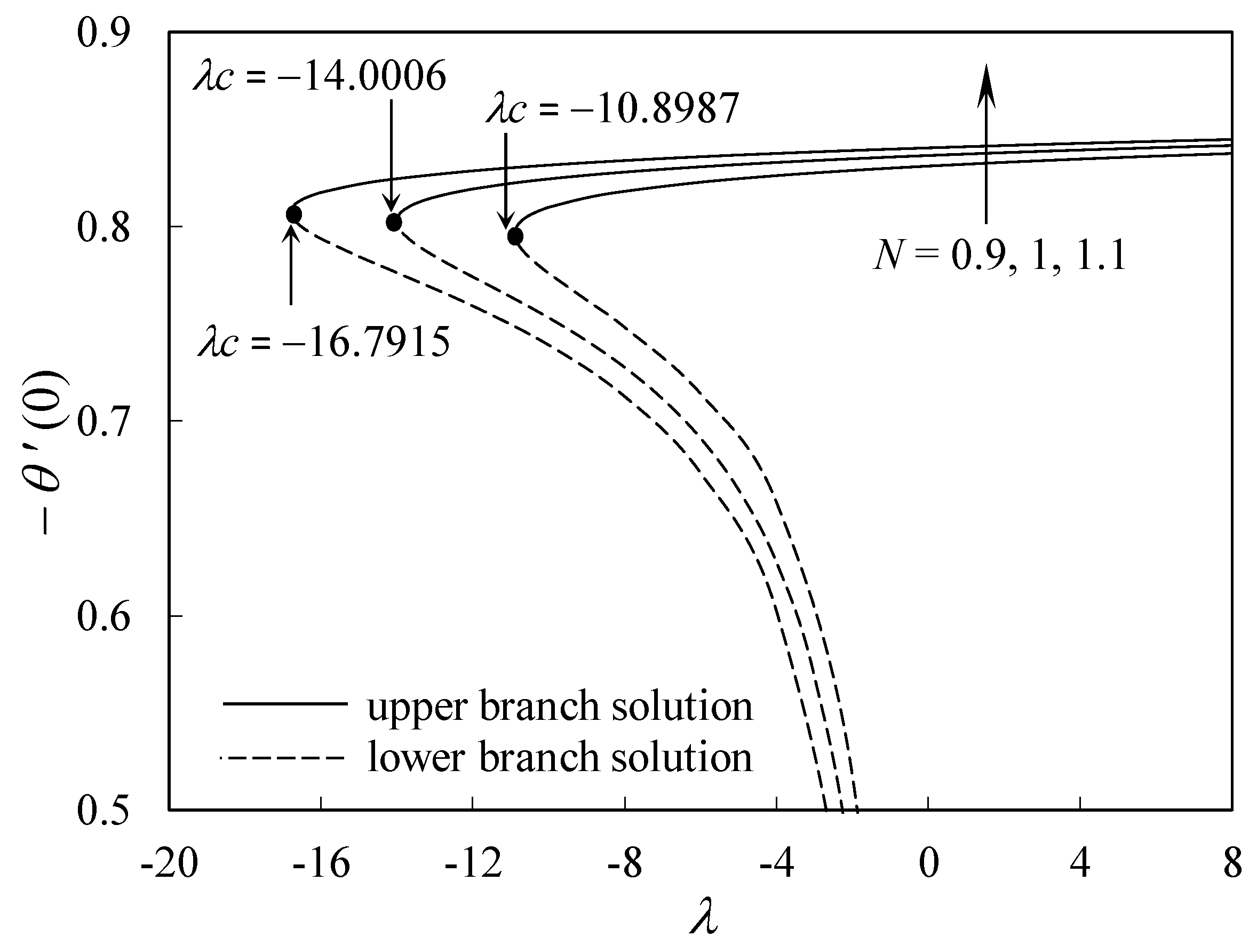
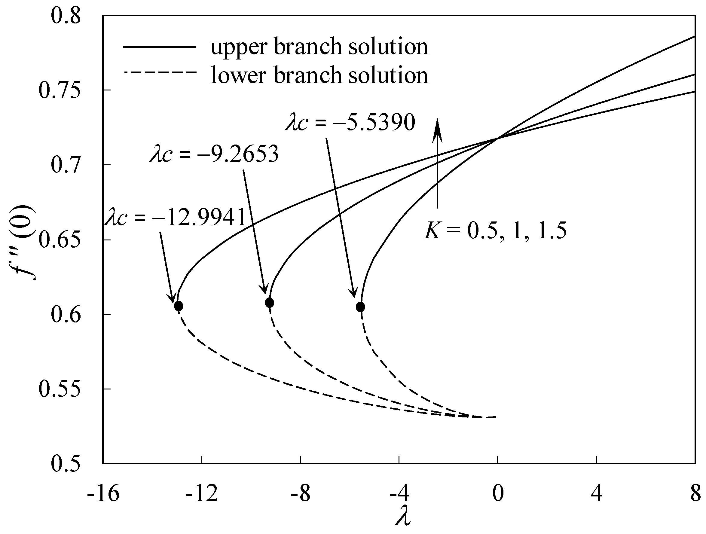
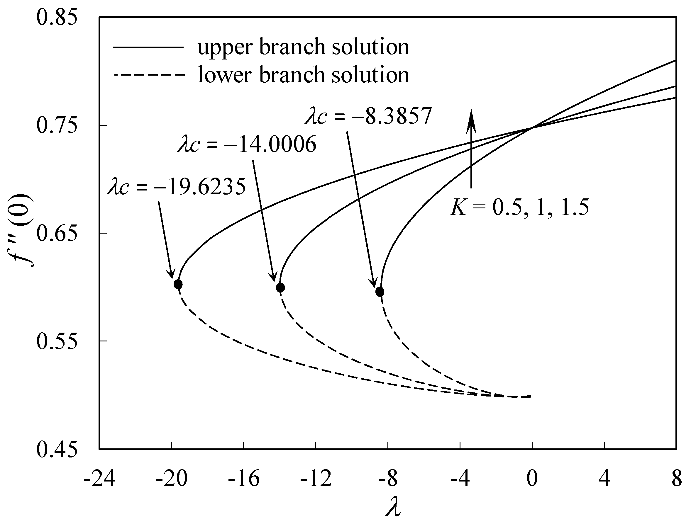
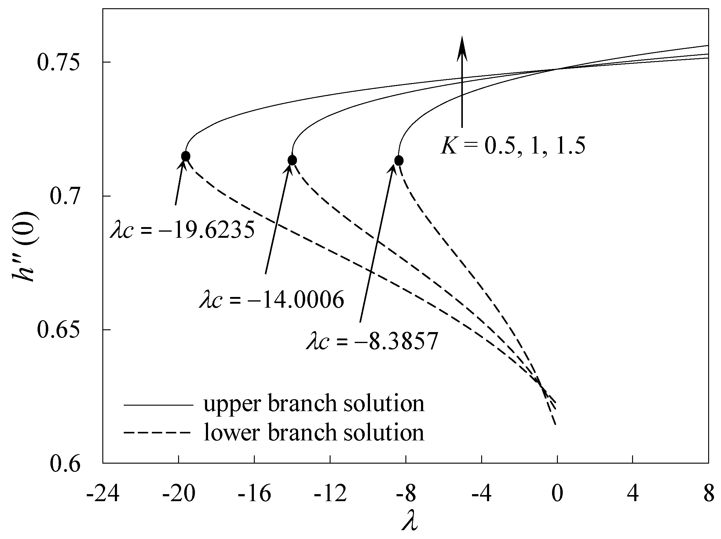
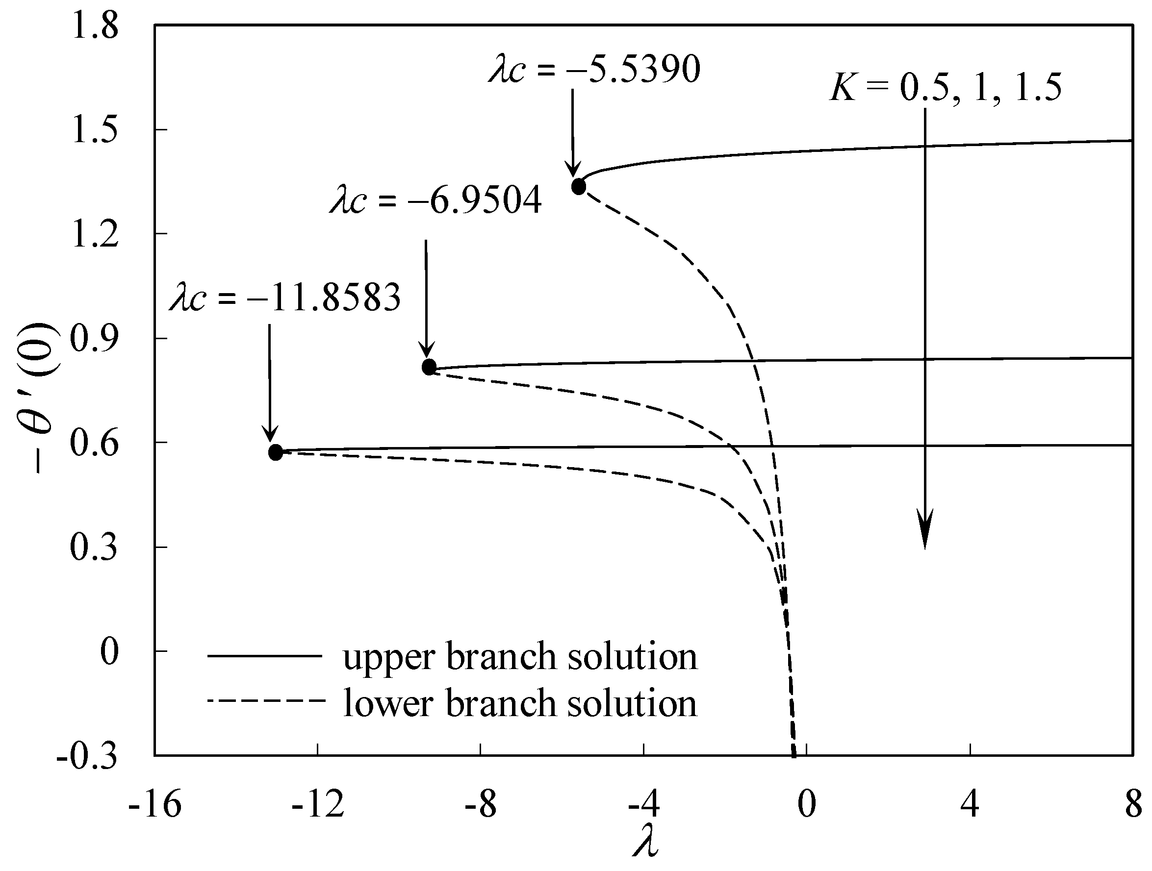
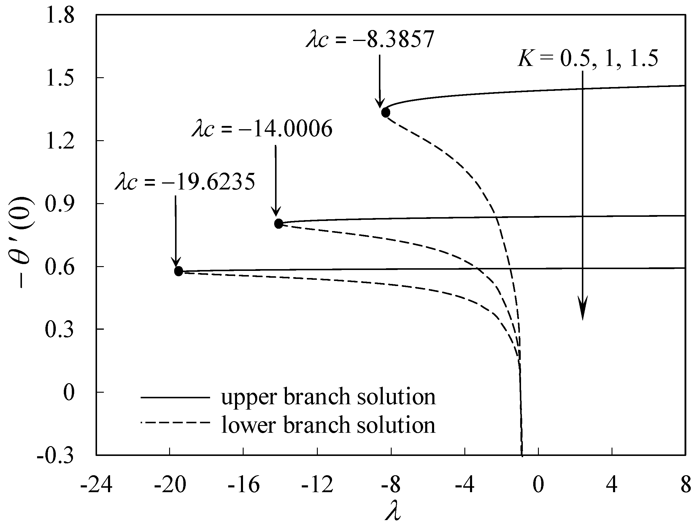
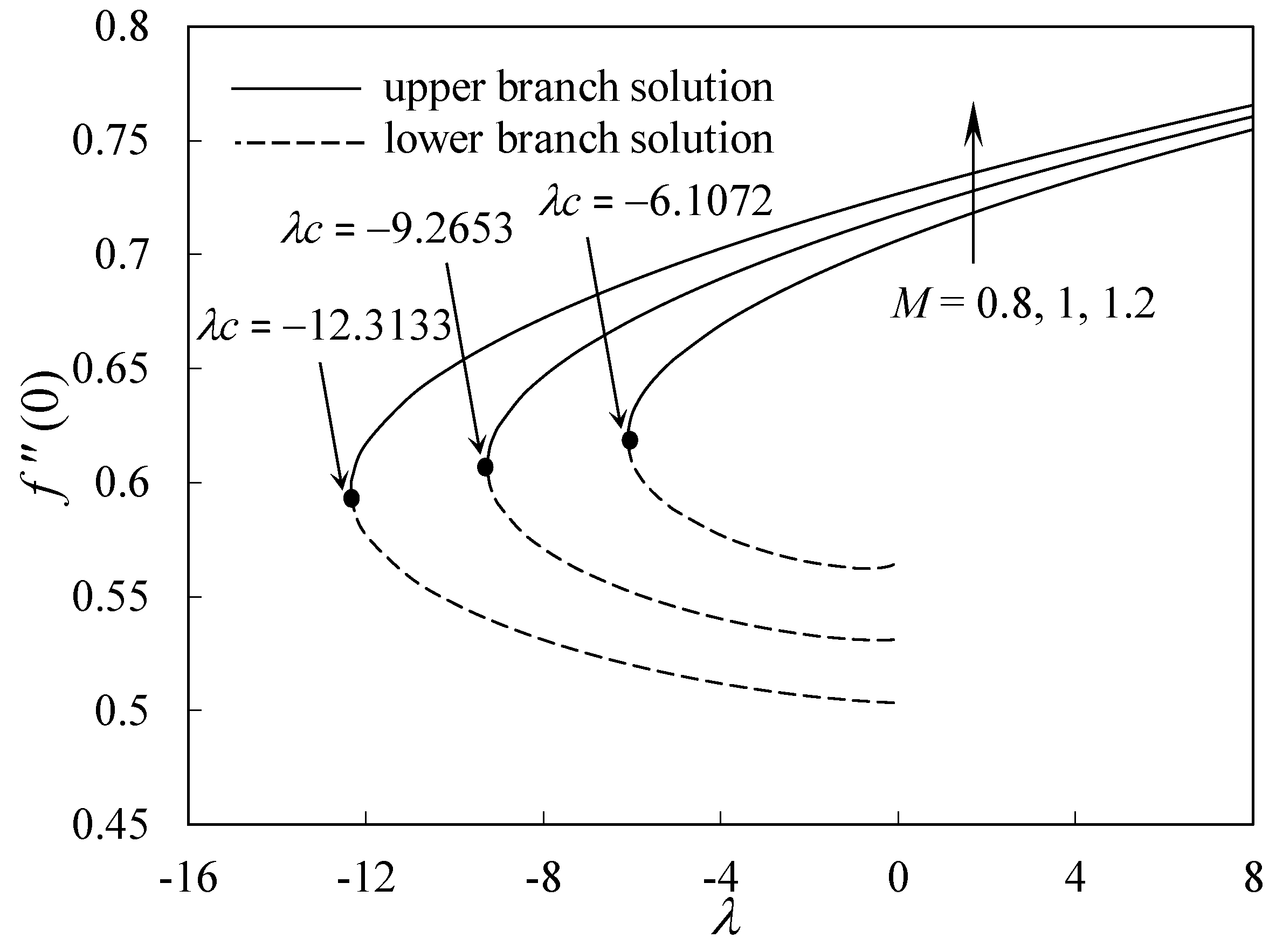
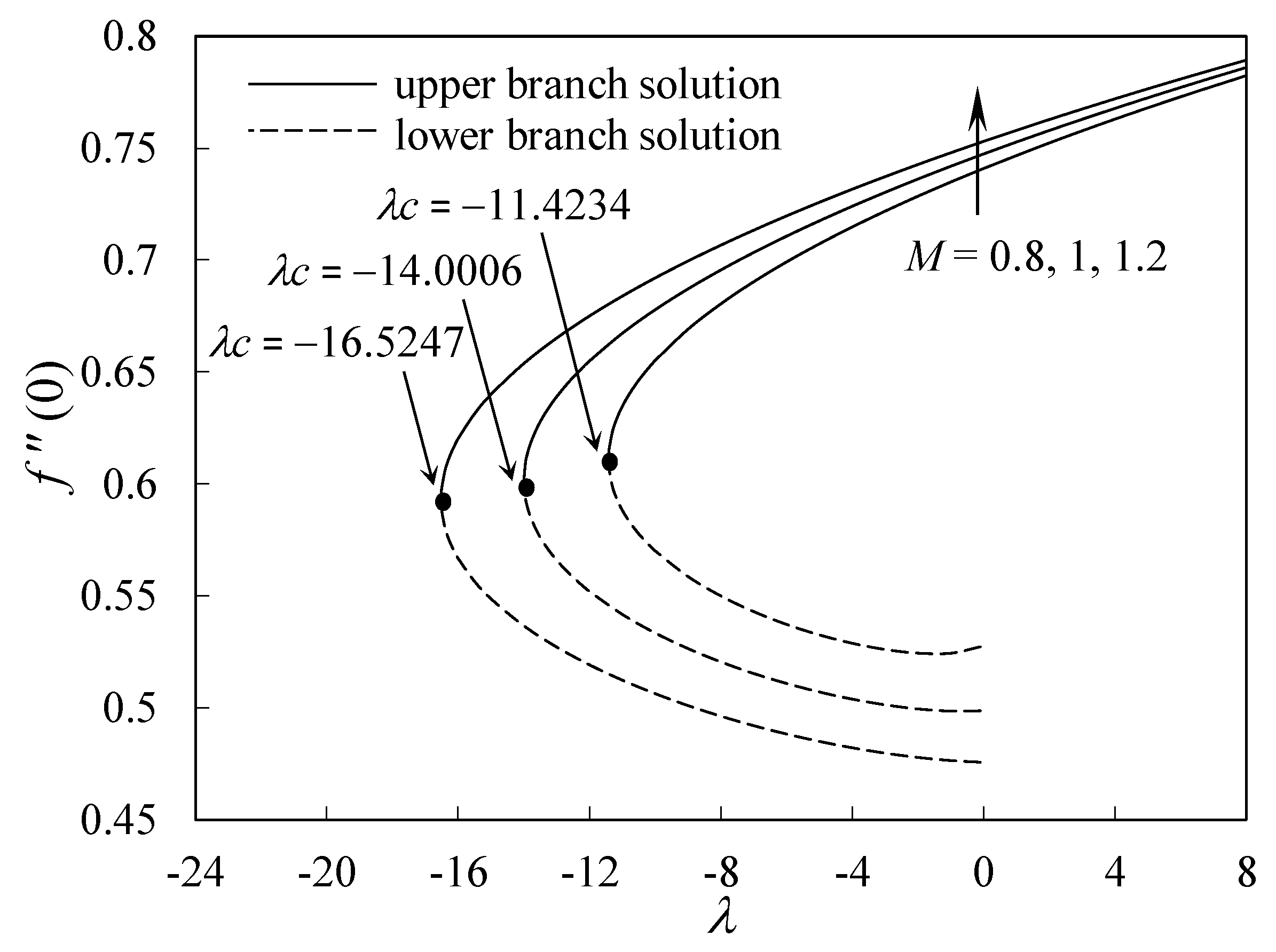
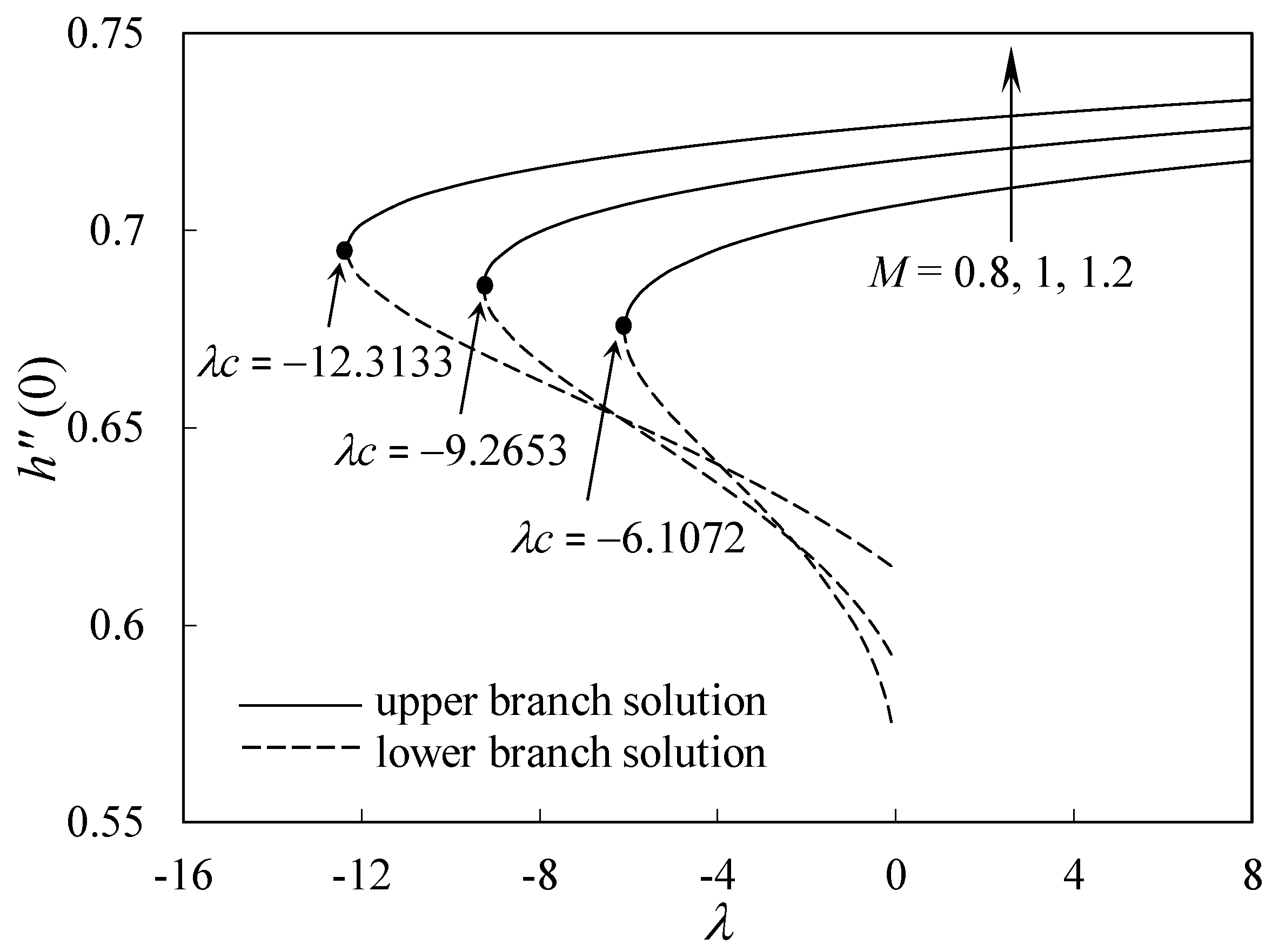
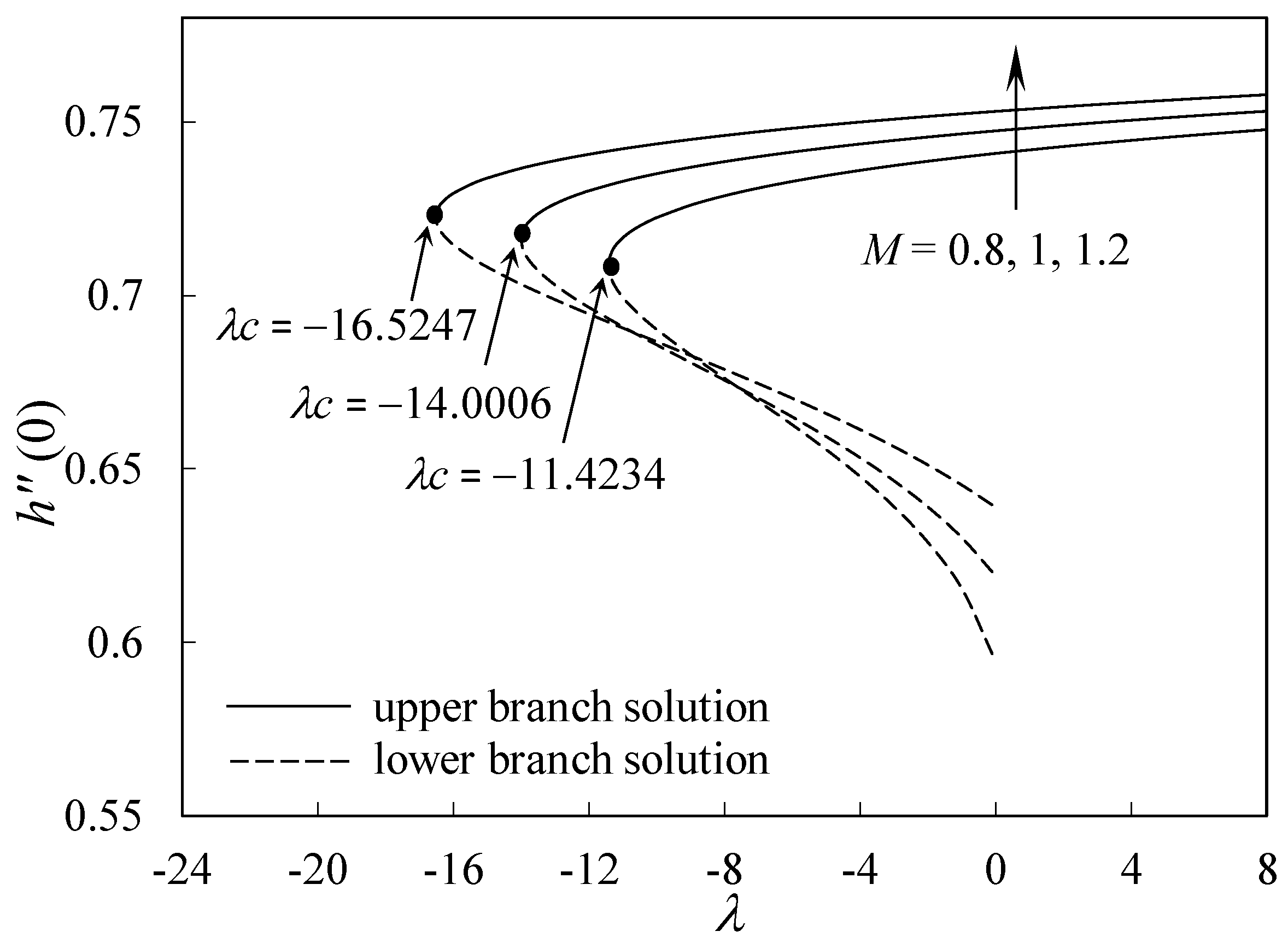
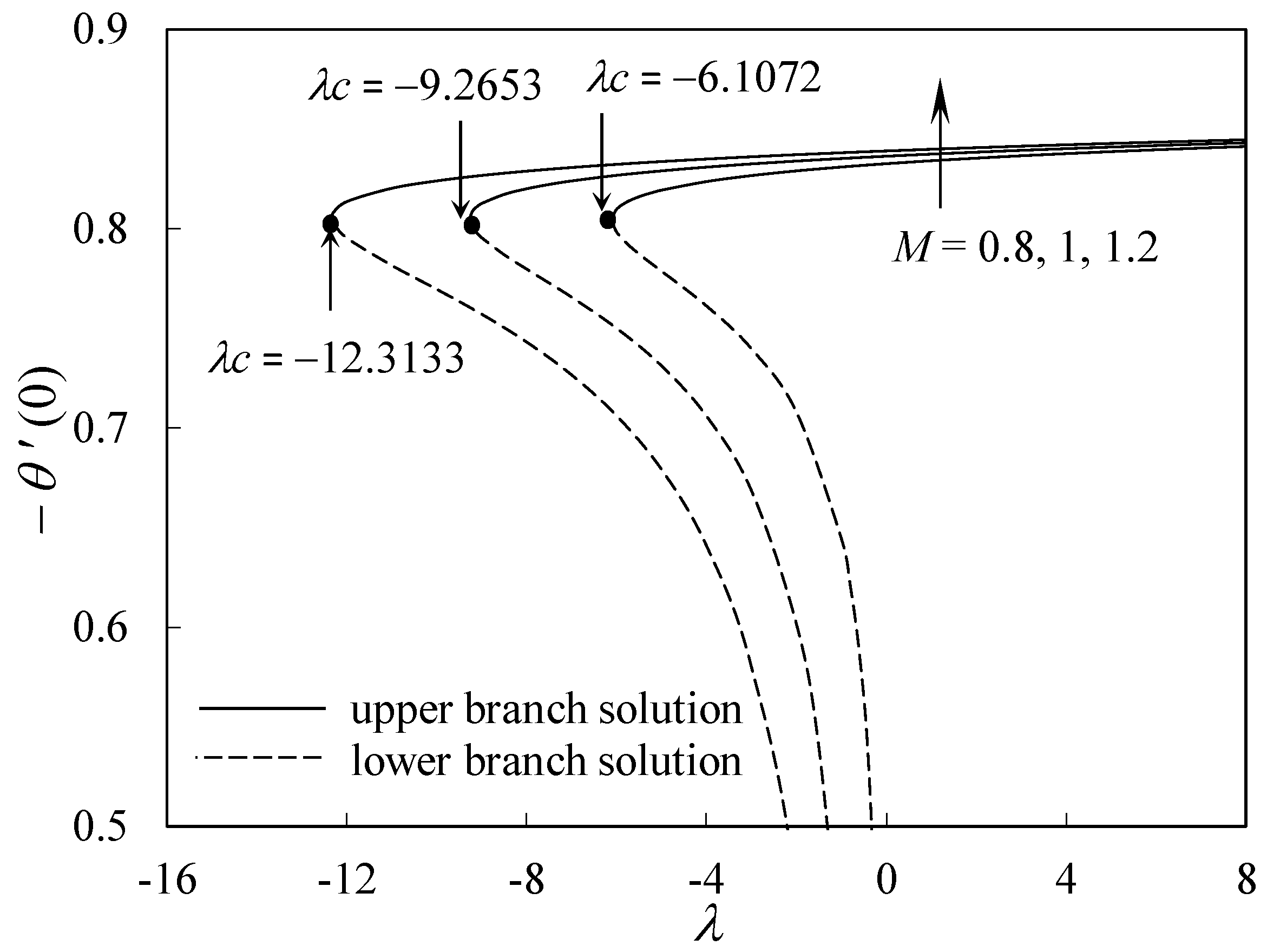
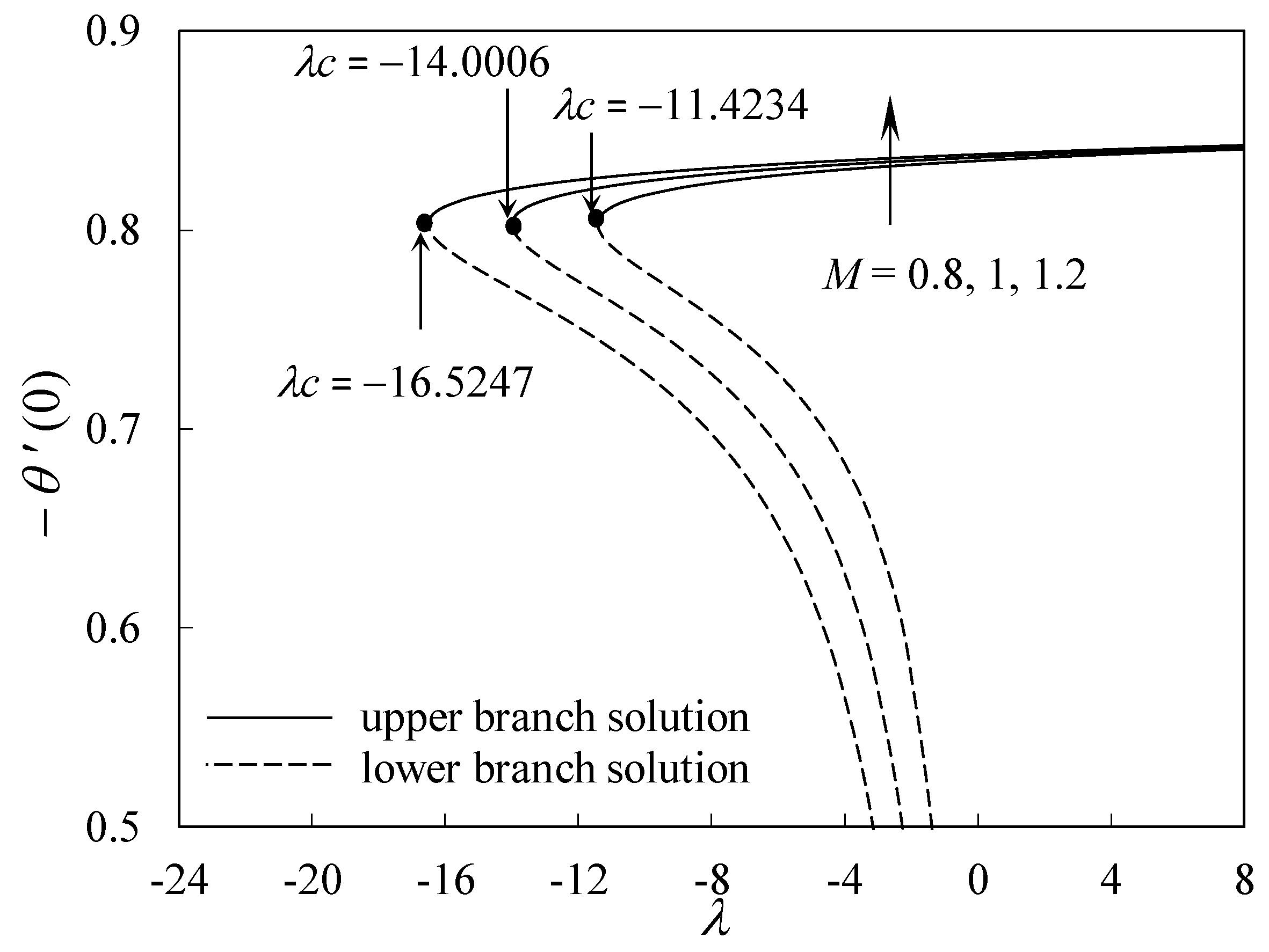
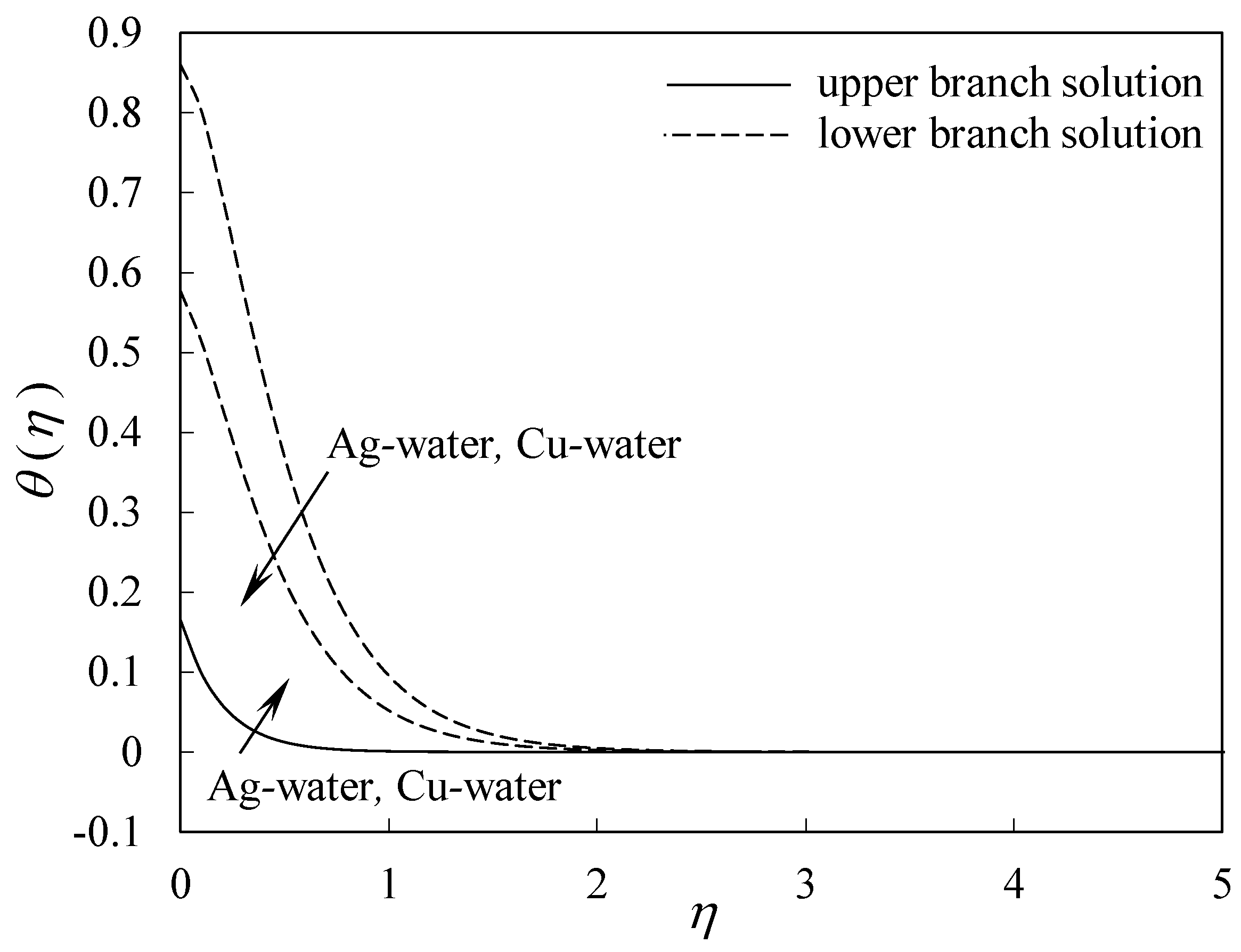
- Dual (upper and lower branch) solutions are found for each value of in the opposing flow region with the solution curves bifurcating at the critical values of , while the lower branch solution could not be continued further to the point where reflected zero.
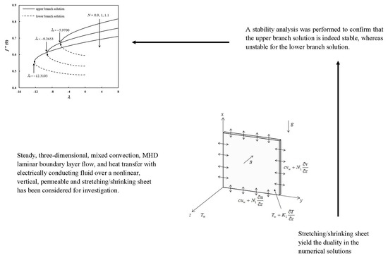
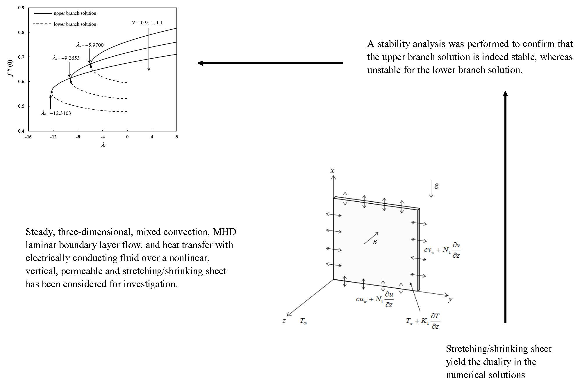
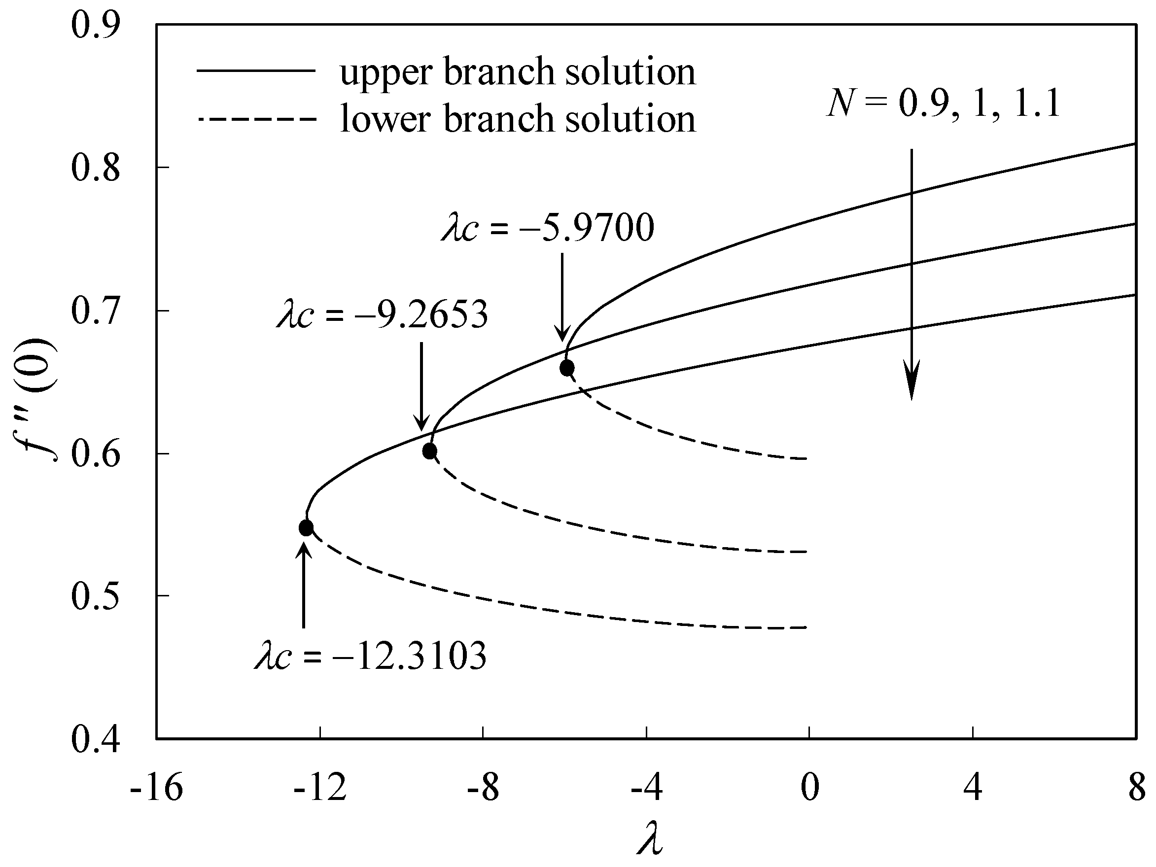
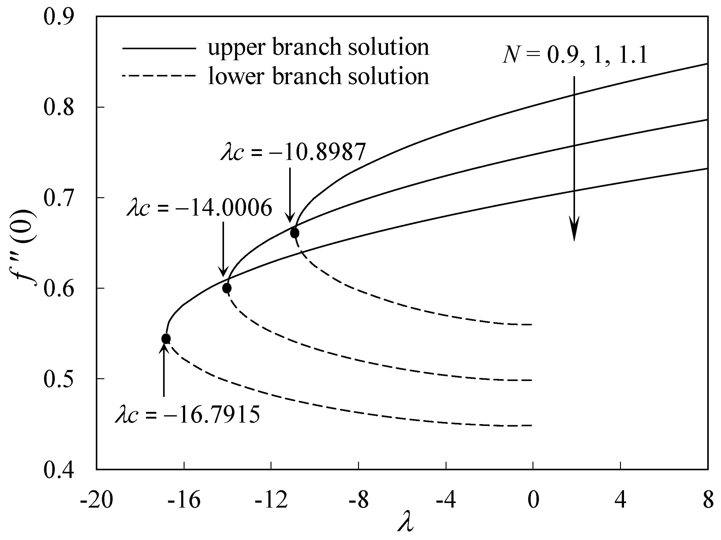
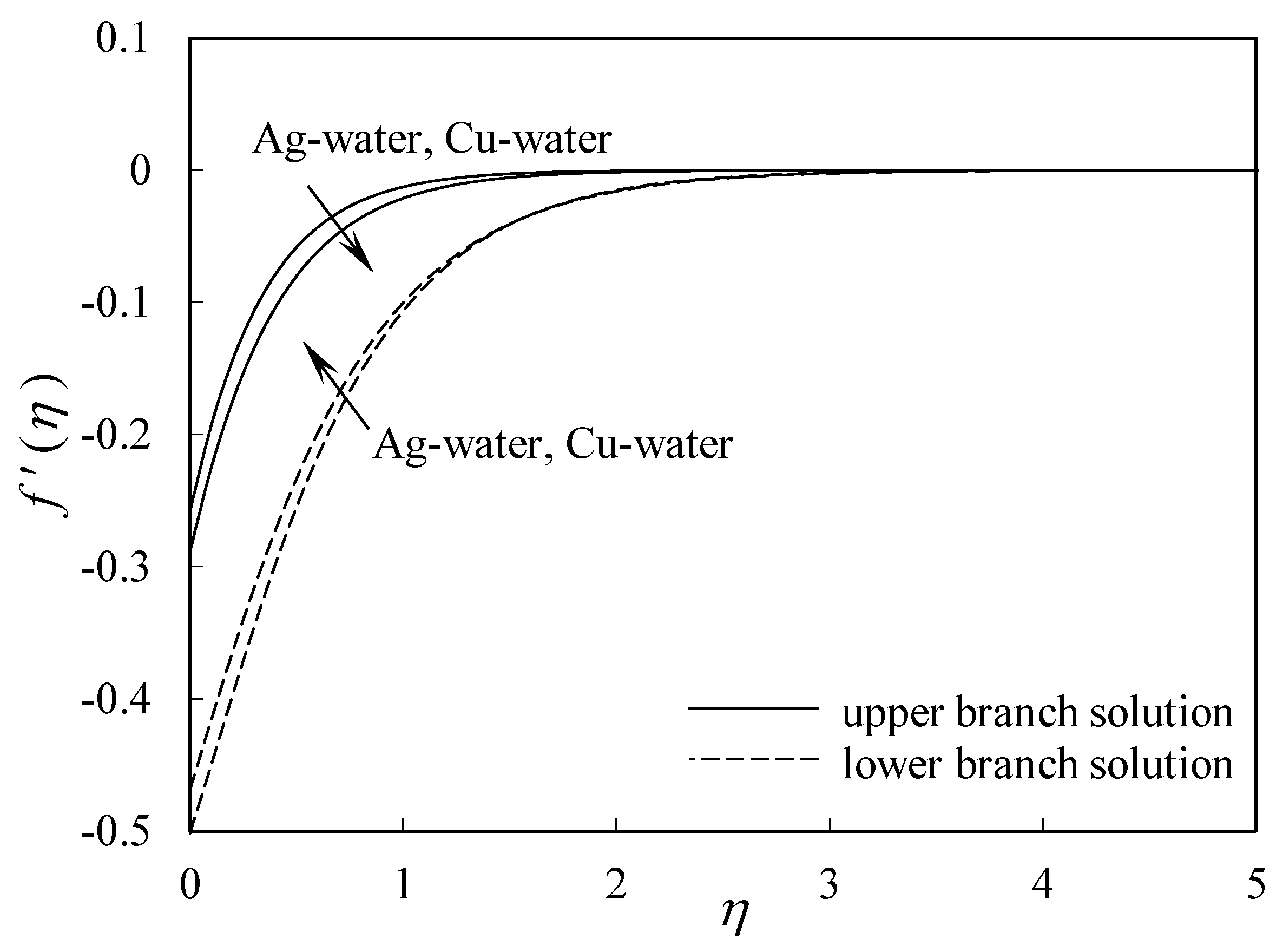
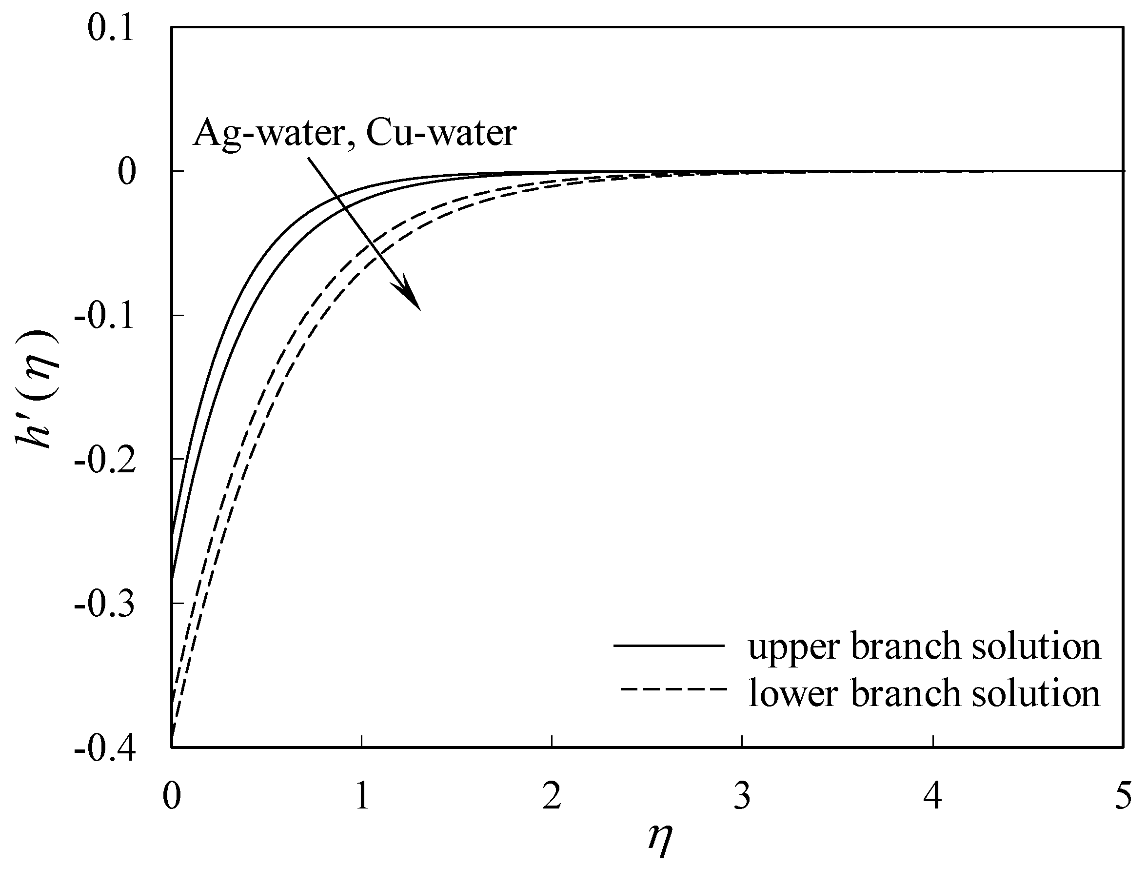
- A stability analysis was performed to confirm that the upper branch solution is indeed stable, whereas unstable for the lower branch solution.
- The value of increases with the increase of N, K, and M, thus, the boundary layer separation can be delayed by increasing the values of the aforementioned parameters.
- Ag-water nanofluid is more capable of delaying the boundary layer separation, in comparison to Cu-water nanofluid.
- Ag-water nanofluid displayed better enhancement for heat transfer, when compared to that for Cu-water nanofluid.
Author Contributions
Acknowledgments
Conflicts of Interest
Nomenclature
| Roman letters | |
| a | positive constant |
| b | constant |
| B0 | constant |
| B | constant magnetic field |
| c | stretching/shrinking parameter |
| Cfx, Cfy | skin friction coefficients along the x and y-directions, respectively |
| f, h | similarity velocity functions |
| f0, h0 | functions |
| g | acceleration due to gravity |
| F, G, H | functions |
| Grx | local Grashof number |
| k | thermal conductivity |
| K0 | constant |
| K1 | thermal slip factor |
| K | temperature slip parameter |
| n | positive constant |
| M | magnetic parameter |
| N0 | constant |
| N1 | velocity slip factor |
| N | velocity slip parameter |
| Nux | local Nusselt number |
| Pr | Prandtl number |
| surface heat flux | |
| Rex, Rey | local Reynolds number along the x and y-directions, respectively |
| s | mass flux parameter |
| t | time |
| T | fluid temperature |
| T0 | characteristic temperature |
| wall temperature | |
| ambient temperature | |
| velocity components along the x-, y- and z-directions, respectively | |
| velocity of the stretching/shrinking surface | |
| mass flux velocity | |
| Cartesian coordinates system | |
| Greek symbols | |
| thermal diffusivity | |
| thermal volumetric coefficient | |
| solid volume fraction of nanoparticles | |
| eigenvalue parameter | |
| smallest eigenvalue parameter | |
| similarity variable | |
| mixed convection parameter | |
| critical value of mixed convection parameter | |
| dynamic viscosity | |
| kinematic viscosity | |
| dimensionless temperature function | |
| function | |
| density of the fluid | |
| electrical conductivity | |
| dimensionless time variable | |
| surface shear stresses denoted as zx and zy, respectively | |
| Subscripts | |
| f | base fluid |
| nf | nanofluid |
| s | solid nanoparticle |
| w | condition on the surface |
| condition outside of boundary layer | |
| Superscript | |
| differentiation with respect to | |
References
- Ramachandran, N.; Chen, T.S.; Armaly, B.F. Mixed convection in stagnation flows adjacent to vertical surfaces. J. Heat Transf. 1988, 110, 373–377. [Google Scholar] [CrossRef]
- Devi, C.D.S.; Takhar, H.S.; Nath, G. Unsteady mixed convection flow in stagnation region adjacent to a vertical surface. Heat Mass Transf. 1991, 26, 71–79. [Google Scholar] [CrossRef]
- Ridha, A.; Curie, M. Aiding flows non-unique similarity solutions of mixed-convection boundary-layer equations. Z. Angew. Math. Phys. 1996, 47, 341–352. [Google Scholar] [CrossRef]
- Merkin, J.H. On dual solutions occurring in mixed convection in a porous medium. J. Eng. Math. 1986, 20, 171–179. [Google Scholar] [CrossRef]
- Merkin, J.H.; Mahmood, T. Mixed convection boundary layer similarity solutions: Prescribed wall heat flux. Z. Angew. Math. Phys. 1989, 40, 51–68. [Google Scholar] [CrossRef]
- Ishak, A.; Merkin, J.H.; Nazar, R.; Pop, I. Mixed convection boundary layer flow over a permeable vertical surface with prescribed wall heat flux. Z. Angew. Math. Phys. 2008, 59, 100–123. [Google Scholar] [CrossRef]
- Deswita, L.; Nazar, R.; Ishak, A.; Ahmad, R.; Pop, I. Mixed convection boundary layer flow past a wedge with permeable walls. Heat Mass Transf. 2010, 46, 1013–1018. [Google Scholar] [CrossRef]
- Roşca, A.V.; Pop, I. Flow and heat transfer over a vertical permeable stretching/shrinking sheet with a second order slip. Int. J. Heat Mass Transf. 2013, 60, 355–364. [Google Scholar] [CrossRef]
- Roşca, N.C.; Pop, I. Mixed convection stagnation point flow past a vertical flat plate with a second order slip: Heat flux case. Int. J. Heat Mass Transf. 2013, 65, 102–109. [Google Scholar] [CrossRef]
- Rahman, M.M.; Merkin, J.H.; Pop, I. Mixed convection boundary-layer flow past a vertical flat plate with a convective boundary condition. Acta Mech. 2015, 226, 2441–2460. [Google Scholar] [CrossRef]
- Ishak, A.; Nazar, R.; Pop, I. Magnetohydrodynamic (MHD) flow of a micropolar fluid towards a stagnation point on a vertical surface. Comput. Math. Appl. 2008, 56, 3188–3194. [Google Scholar] [CrossRef] [Green Version]
- Makinde, O.D.; Chinyoka, T. MHD transient flows and heat transfer of dusty fluid in a channel with variable physical properties and Navier slip condition. Comput. Math. Appl. 2010, 60, 660–669. [Google Scholar] [CrossRef]
- Gireesha, B.J.; Mahanthesh, B.; Rashidi, M.M. MHD boundary layer heat and mass transfer of a chemically reacting Casson fluid over a permeable stretching surface with non-uniform heat source/sink. Int. J. Ind. Math. 2015, 7, 247–260. [Google Scholar]
- Ishak, A.; Nazar, R.; Arifin, N.M.; Pop, I. Dual solutions in magnetohydrodynamic mixed convection flow near a stagnation-point on a vertical surface. J. Heat Transf. 2007, 129, 1212–1216. [Google Scholar] [CrossRef]
- Ali, F.M.; Nazar, R.; Arifin, N.M.; Pop, I. MHD mixed convection boundary layer flow toward a stagnation point on a vertical surface with induced magnetic field. J. Heat Transf. 2011, 133, 022502. [Google Scholar] [CrossRef]
- Sandeep, N.; Sulochana, C.; Sugunamma, V. Radiation and magnetic field effects on unsteady mixed convection flow over a vertical stretching/shrinking surface with suction/injection. Ind. Eng. Lett. 2015, 5, 127–136. [Google Scholar]
- Sharada, K.; Shankar, B. Three-dimensional MHD mixed convection Casson fluid flow over an exponential stretching sheet with the effect of heat generation. Br. J. Math. Comput. Sci. 2016, 19, 1–8. [Google Scholar] [CrossRef]
- Sivasankaran, S.; Niranjan, H.; Bhuvaneswari, M. Chemical reaction, radiation and slip effects on MHD mixed convection stagnation-point flow in a porous medium with convective boundary condition. Int. J. Numer. Method Heat Fluid Flow 2017, 27, 454–470. [Google Scholar] [CrossRef]
- Wong, K.V.; De Leon, O. Applications of nanofluids: Current and future. Adv. Mech. Eng. 2010, 2, 519659. [Google Scholar] [CrossRef]
- Saidur, R.; Leong, K.Y.; Mohammad, H. A review on applications and challenges of nanofluids. Renew. Sust. Energy Rev. 2011, 15, 1646–1668. [Google Scholar] [CrossRef]
- Eastman, J.A.; Choi, S.U.S.; Li, S.; Yu, W. Thompson LJ Anomalously increased effective thermal conductivities of ethylene glycol-based nanofluids containing copper nanoparticles. Appl. Phys. Lett. 2001, 78, 718–720. [Google Scholar] [CrossRef]
- Liu, M.S.; Lin, M.C.C.; Tsai, C.Y.; Wang, C.C. Enhancement of thermal conductivity with Cu for nanofluids using chemical reduction method. Int. J. Heat Mass Transf. 2006, 49, 3028–3033. [Google Scholar] [CrossRef]
- Hwang, Y.J.; Ahn, Y.C.; Shin, H.S.; Lee, C.G.; Kim, G.T.; Park, H.S.; Lee, J.K. Investigation on characteristics of thermal conductivity enhancement of nanofluids. Curr. Appl. Phys. 2006, 6, 1068–1071. [Google Scholar] [CrossRef]
- Tiwari, R.K.; Das, M.K. Heat transfer augmentation in a two-sided lid-driven differentially heated square cavity utilizing nanofluids. Int. J. Heat Mass Transf. 2007, 50, 2002–2018. [Google Scholar] [CrossRef]
- Buongiorno, J. Convective transport in nanofluids. J. Heat Transf. 2006, 28, 240–250. [Google Scholar] [CrossRef]
- Yasin, M.H.M.; Arifin, N.M.; Nazar, R.; Ismail, F.; Pop, I. Mixed convection boundary layer flow on a vertical surface in a porous medium saturated by a nanofluid with suction or injection. J. Math. Stat. 2013, 9, 119–128. [Google Scholar] [CrossRef]
- Pal, D.; Mandal, G.; Vajravalu, K. Mixed convection stagnation-point flow of nanofluids over a stretching/shrinking sheet in a porous medium with internal heat generation/absorption. Commun. Numer. Anal. 2015, 2015, 30–50. [Google Scholar] [CrossRef]
- Pal, D.; Mandal, G. Mixed convection-radiation on stagnation-point flow of nanofluids over a stretching/shrinking sheet in a porous medium with heat generation and viscous dissipation. J. Pet. Sci. Eng. 2015, 126, 16–25. [Google Scholar] [CrossRef]
- Mahdy, A. Unsteady mixed convection boundary layer flow and heat transfer of nanofluids due to stretching sheet. Nucl. Eng. Des. 2012, 249, 248–255. [Google Scholar] [CrossRef]
- Abdullah, A.A.; Ibrahim, F.S.; Gawad, A.A.; Batyyb, A. Investigation of unsteady mixed convection flow near the stagnation point of a heated vertical plate embedded in a nanofluid-saturated porous medium by self-similar. Am. J. Energy Eng. 2015, 3, 42–51. [Google Scholar] [CrossRef]
- Oyelakin, I.S.; Mondal, S.; Sibanda, P. Unsteady mixed convection in nanofluid flow through a porous medium with thermal radiation using the Bivariate Spectral Quasilinearization method. J. Nanofluids 2017, 6, 273–281. [Google Scholar] [CrossRef]
- Yazdi, M.; Moradi, A.; Dinarvand, S. MHD mixed convection stagnation-point flow over a stretching vertical plate in porous medium filled with a nanofluid in the presence of thermal radiation. Arab. J. Sci. Eng. 2014, 39, 2251–2261. [Google Scholar] [CrossRef]
- Haroun, N.A.; Sibanda, P.; Mondal, S.; Motsa, S.S. On unsteady MHD mixed convection in a nanofluid due to a stretching/shrinking surface with suction/injection using the spectral relaxation method. Bound. Value Probl. 2015, 2015, 24. [Google Scholar] [CrossRef]
- Mustafa, I.; Javed, T.; Majeed, A. Magnetohydrodynamic (MHD) mixed convection stagnation point flow of a nanofluid over a vertical plate with viscous dissipation. Can. J. Phys. 2015, 93, 1365–1374. [Google Scholar] [CrossRef]
- Mahanthesh, B.; Gireesha, B.J.; Gorla, R.S.; Makinde, O.D. Magnetohydrodynamic three-dimensional flow of nanofluids with slip and thermal radiation over a nonlinear stretching sheet: A numerical study. Neural Comput. Appl. 2016, 1–11. [Google Scholar] [CrossRef]
- Noghrehabadi, A.; Pourrajab, R.; Ghalambaz, M. Effect of partial slip boundary condition on the flow and heat transfer of nanofluids past stretching sheet prescribed constant wall temperature. Int. J. Therm. Sci. 2012, 54, 253–261. [Google Scholar] [CrossRef]
- Ibrahim, W.; Shankar, B. MHD boundary layer flow and heat transfer of a nanofluid past a permeable stretching sheet with velocity, thermal and solutal slip boundary conditions. Comput. Fluids 2013, 75, 1–10. [Google Scholar] [CrossRef]
- Hayat, T.; Imtiaz, M.; Alsaedi, A.; Kutbi, M.A. MHD three-dimensional flow of nanofluid with velocity slip and nonlinear thermal radiation. J. Magn. Magn. Mater. 2015, 396, 31–37. [Google Scholar] [CrossRef]
- Roşca, N.C.; Roşca, A.V.; Aly, E.H.; Pop, I. Semi-analytical solution for the flow of a nanofluid over a permeable stretching/shrinking sheet with velocity slip using Buongiorno’s mathematical model. Eur. J. Mech. B-Fluid 2016, 58, 39–49. [Google Scholar] [CrossRef]
- Oztop, H.F.; Abu-Nada, E. Numerical study of natural convection in partially heated rectangular enclosures filled with nanofluids. Int. J. Heat Fluid Flow 2008, 29, 1326–1336. [Google Scholar] [CrossRef]
- Das, S.; Jana, R.N. Natural convective magneto-nanofluid flow and radiative heat transfer past a moving vertical plate. Alexandria Eng. J. 2015, 54, 55–64. [Google Scholar] [CrossRef]
- Gul, A.; Khan, I.; Shafie, S. Radiation and heat generation effects in MHD mixed convection flow of nanofluids. Therm. Sci. 2016. [Google Scholar] [CrossRef]
- Garnett, J.M. Colours in metal glasses and in metallic films. Philos. Trans. R. Soc. A 1904, 203, 385–420. [Google Scholar] [CrossRef]
- Brinkman, H.C. The viscosity of concentrated suspensions and solutions. J. Chem. Phys. 1952, 20, 571. [Google Scholar] [CrossRef]
- Maiga, S.E.B.; Palm, S.J.; Nguyen, C.T.; Roy, G.; Galanis, N. Heat transfer enhancement by using nanofluids in forced convection flows. Int. J. Heat Fluid Flow 2005, 26, 530–546. [Google Scholar] [CrossRef]
- Weidman, P.D.; Kubitschek, D.G.; Davis, A.M.J. The effect of transpiration on self-similar boundary layer flow over moving surfaces. Int. J. Eng. Sci. 2006, 44, 730–737. [Google Scholar] [CrossRef]
- Harris, S.D.; Ingham, D.B.; Pop, I. Mixed convection boundary-layer flow near the stagnation point on a vertical surface in a porous medium: Brinkman model with slip. Transp. Porous Med. 2009, 77, 267–285. [Google Scholar] [CrossRef]
- Shampine, L.F.; Reichelt, M.W.; Kierzenka, J. Solving Boundary Value Problems for Ordinary Differential Equations in MATLAB with bvp4c. 2010. Available online: http://www.mathworks.com/bvp_tutorial (accessed on 25 January 2018).
- Jain, S.; Choudhary, R. Thermophoretic MHD flow and non-linear radiative heat transfer with convective boundary conditions over a non-linearly stretching sheet. arXiv, 2017; arXiv:1702.02039. [Google Scholar]


| Physical Properties | Water | Cu | Ag |
|---|---|---|---|
| (J kg−1 K−1) | 4179 | 385 | 235 |
| (k gm−1) | 997.1 | 8933 | 10,500 |
| (Wm−1 K−1) | 0.613 | 400 | 429 |
| (K−1) | 21 | 1.67 | 1.89 |
| (Sm−1) | 5.5 10−6 | 59.6 106 | 6.3 107 |
| M | n | Mahanthesh et al. [35] | Jain and Choudhary [49] | Present |
|---|---|---|---|---|
| 0 | 1 | −1.41421 | −1.419135111 | −1.414214 |
| 3 | −2.29719 | −2.301331346 | −2.297186 | |
| 2 | 1 | – | −2.000000000 | −2.000000 |
| 3 | – | −2.701221616 | −2.701216 |
| N | K | M | (Upper Branch) | (Lower Branch) | |
|---|---|---|---|---|---|
| 1 | 1 | 1 | −9 | 3.4985 | −0.2172 |
| −9.2 | 1.8120 | −0.1051 | |||
| 1 | 1 | 0.8 | −6 | 5.0945 | −0.1339 |
| −6.1 | 3.3007 | −0.0133 | |||
| 1 | 0.5 | 1 | −5 | 5.2992 | −0.4028 |
| −5.5 | 1.8051 | −0.1048 | |||
| 0.9 | 1 | 1 | −5 | 8.9037 | −0.4313 |
| −5.9 | 5.1995 | −0.1139 |
© 2018 by the authors. Licensee MDPI, Basel, Switzerland. This article is an open access article distributed under the terms and conditions of the Creative Commons Attribution (CC BY) license (http://creativecommons.org/licenses/by/4.0/).
Share and Cite
Jamaludin, A.; Nazar, R.; Pop, I. Three-Dimensional Magnetohydrodynamic Mixed Convection Flow of Nanofluids over a Nonlinearly Permeable Stretching/Shrinking Sheet with Velocity and Thermal Slip. Appl. Sci. 2018, 8, 1128. https://doi.org/10.3390/app8071128
Jamaludin A, Nazar R, Pop I. Three-Dimensional Magnetohydrodynamic Mixed Convection Flow of Nanofluids over a Nonlinearly Permeable Stretching/Shrinking Sheet with Velocity and Thermal Slip. Applied Sciences. 2018; 8(7):1128. https://doi.org/10.3390/app8071128
Chicago/Turabian StyleJamaludin, Anuar, Roslinda Nazar, and Ioan Pop. 2018. "Three-Dimensional Magnetohydrodynamic Mixed Convection Flow of Nanofluids over a Nonlinearly Permeable Stretching/Shrinking Sheet with Velocity and Thermal Slip" Applied Sciences 8, no. 7: 1128. https://doi.org/10.3390/app8071128