A Running Reference Analysis Method to Greatly Improve Optical Backscatter Reflectometry Strain Data from the Inside of Hardening and Shrinking Materials

Abstract

Due to the increasing ease of use and the superiority of the results, distributed strain measurements, utilizing Optical Backscatter Reflectometry (OBR), have become more important and widespread over the last few years. Strains are calculated from the difference between an actual optical Raleigh backscattering measurement and an initial reference value. However, under certain physical conditions, e.g., pinching or microbending of the optical fiber, no meaningful strain values are yielded by the commonly-used method to analyze OBR data. Such conditions were experienced in this study where the optical fiber was embedded into hardening epoxy for measuring shrinkage due to curing. In this work, it is shown that a new data analysis method called the “running reference analysis method” can overcome such obstacles and deliver meaningful strain values in circumstances in which the traditional method fails. In the new approach, each measurement is compared to the previous measurement, and the strain differences are added up to the absolute strain value. This method does not require a new experimental technique and will also work on old measurement files. It is also useful for other types of (OBR) strain measurements that contain many outliers and is not restricted to the investigation of cured epoxy.

1. Introduction

Many important large infrastructure components are created by pouring a liquid material (e.g., cement or a polymer) into a mold and simply letting the material harden or cure. Examples may be bridges, wind turbine blades or electrical transformers. Volume shrinkage of such materials during the curing process is a well-known phenomenon. Good measurements of the shrinkage are essential for understanding and modeling the materials’ behavior. For example, the durability of concrete structures is dependent on the formation of cracks, which develop due to such volume reductions during the hardening process [1,2].

A variety of techniques exist to measure the volume shrinkage of a material while it is hardening. This introductory overview concentrates on cementitious and polymer materials, but the methods should be applicable to many other material classes.

The average shrinkage can be determined by simply measuring the outer dimensions or the buoyancy of a sample [3,4]. Rheometry [5,6], pycnometry [7,8], dilatometry [9,10,11] or thermo-mechanical analysis [12,13] are other, more complicated methods to measure the average shrinkage of a material. Another method is the tracking of the position of embedded objects by various means [14,15]. However, the strain information these methods yield is limited. The samples as a whole are the subjects of the measurement, and thus, the average strain is determined. In addition, often, the sample size that can be used in such experiments is rather small. This may reflect an unrealistic picture of hardening processes in real-world technical applications, since the production and dissipation of heat or the diffusion of water out of a structure are size and probably geometry dependent [16,17].

Digital image correlation tracks surface structures and allows one to determine two-dimensional local shrinkage on the surface of a sample [18,19]. While this technique yields much more detailed information than the above methods, it can only be applied to rather small samples, with sizes of some centimeters.

The biggest disadvantage of all these techniques is that they are incapable of measuring the strain inside the structure. Especially for large structures, the knowledge about internal strain gradients may be of high importance to determine overall structural parameters.

Traditional strain gauges may be placed directly into the still liquid material to measure internal strain [20,21,22]. However, this method yields just punctiform strain information, at the location of the strain gauge.

Another method to measure internal strains is the use of optical Fibers with Bragg Gratings (FBGs) [23,24,25,26]. Optical fibers are resistant to most environments, which predestine them for embedding in many kinds of materials. They are easy to apply and have good resolution.

Strains are measured by sending laser light through the fiber. One frequency of the light is reflected at the Bragg grating, and the reflected light is recorded. When the component to which the fiber is attached gets strained, the fiber strains as well. This causes the Bragg grating to change length, and a different frequency is reflected. By comparing the recorded frequencies of the reflected light of the initial condition and the loaded condition, the strain at the Bragg grating can be calculated, and a measurement is done. However, as for strain gauges, strain concentrations or generally strain gradients cannot be measured well with Bragg gratings. The possibility to measure strain gradients over the length of an FBG has been reported [27,28,29,30]. However, the length of such gratings is rather short, less then 25 mm in the cited works, and many FBGs have to be applied to cover the strain gradient in large structures.

Measuring strain with optical fibers using an Optical Backscatter Reflectometer (OBR) has removed the above-mentioned problems. The OBR method can use regular communication fibers. Laser light is sent into the fiber, and Rayleigh backscattered light will be analyzed to calculate strain in the fiber. Backscattering happens at irregularities of the fiber material. This means strains can be measured along the entire length of the fiber, thus allowing one to monitor large structures. It is basically a long array of many individual strain gauges. OBR is a relatively new technique and has been used so far in structures to, e.g., determine strain fields under load, assess crack development or in general structural health monitoring [31,32,33,34,35,36,37,38].

To the authors knowledge, OBR has not been used so far to determine the internal shrinkage of, e.g., large cementitious or polymer structures. This may be due to the forces acting on the fiber during the curing process, which in return deteriorate the backscattered signal greatly, and thus, only noise is extracted in traditional OBR analysis. This issue will be discussed below, in addition to how OBR works in detail. The main part of this article discusses how a new method to analyze the data can tremendously improve the obtained strain information.

The need to improve the OBR analysis came out of a project to analyze the curing behavior of epoxy in large molds. Epoxy is a two-component polymer. The two components are mixed, and the epoxy is cast into a form. The two components react with each other, forming chemical bonds. This creates a network of bonds, and the epoxy turns into a solid block of material. The curing reaction is exothermic, i.e., heat is released. The forming of the bonds reduces the volume of the material, the so-called cure shrinkage. This shrinkage causes also strains in the material. The curing process is complex, being different at different locations inside a cast component, while the whole block exhibits an average shrinkage.

This research is described in detail in [17]. Hence, the paper at hand does not focus on the curing characteristics, but on the challenges of measuring the strain distribution along the fiber inside the hardening material. Solutions to the encountered measurement challenges are described here. The solutions will be useful for many applications of the OBR technique where local forces act on the fiber and high strain gradients occur.

2. Experimental Setup

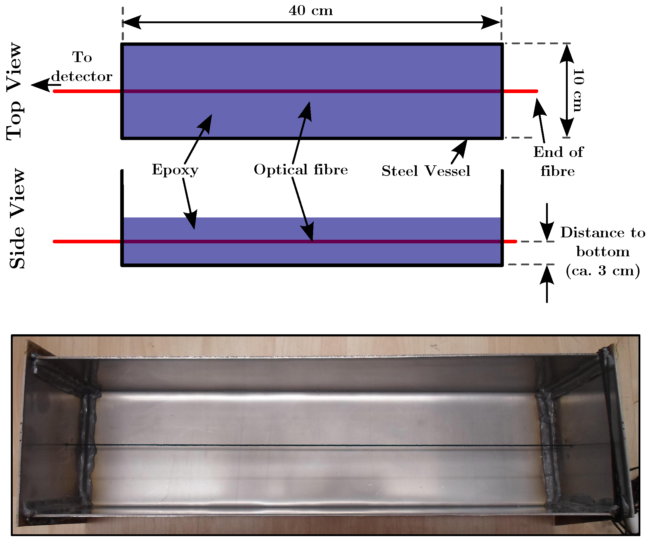
Experiments were performed to monitor the cure shrinkage of epoxy. A simple brick-shaped epoxy block was chosen for the study. Liquid epoxy was poured into a metal mold to a height of 6 cm. The mold was 10 cm high and had a rectangular bottom of $40\times 10$ cm. The setup is shown in Figure 1. The epoxy was a mixture of ten parts Epikote Resin MGS RIMR 135 and three parts Epikure Curing Agent MGS RIMH 137 [39]. The two components reacted with each other and turned into a solid block after about five hours. More details about the reaction are described in [39].

The single-mode optical fibre from OFS Fitel, LLC with an operating wavelength of 1550 nm, core, clad and coating diameters of respectively 6500 nm, 0.125 mm and 0.155 mm, Pyrocoat^® coating and an operating temperature between −65 to +300 degrees Celsius (visualized by a black thread in Figure 1) was put into the mould before pouring the epoxy. The fibre was held in a horizontal position in the middle of the epoxy (about 3 cm high) by leading it through two small holes in the mold. Rubber, applied from the inside, was used to hold the fibre in place and prevent the epoxy from seeping through the holes. An “OBR 4600” from Luna Instruments [40] was used to detect the OBR signal with the following settings: (virtual) gauge length = 1.0 cm, sensor spacing = 1 mm, strain resolution < 30 ppm [41].

Measurements were taken with the OBR in every 15 min for temperatures below and every 3 min above 40 degrees Celsius. A single measurement took approximately 5 s. The temperature was determined with Radial Glass NTC Thermistors, which were embedded into the epoxy. These were encapsulated in glass, have 10 kΩ resistance at 25 degrees Celsius and have a temperature range from −40–+250 degrees Celsius. See [17] for details of the temperature measurements setup. Initially, the optical fiber is surrounded by liquid epoxy. Strains do not exist in the liquid, and no strains are transferred to the fiber. This state is referred to a zero strain, and it is the same strain along the length of the fiber. However, the fiber will experience the increased temperature due to the exothermic reaction heat of the epoxy. The temperature increase leads to an apparent positive strain along the length of the fiber. It is important that this signal due to elevated temperatures is not interpreted as actual strain onto the fiber.

The epoxy will obtain an increase in viscosity as more chemical bonds form. Gradually, the epoxy will become a solid material. At some point in the curing process, the epoxy will adhere to the optical fiber and be able to transfer forces and strain into the fiber. More details about the experimental setup and the stages of the curing process are presented in [17].

3. Fundamental OBR Principles and the Traditional Method to Analyze the Data

To measure strain profiles along an optical fiber, Optical Time Domain Reflectometry (OTDR) or Optical Frequency Domain Reflectometry (OFDR) are utilized. Time of flight measurements of a laser pulse are usually used in OTDR to calculate the position of a signal along the fiber. In OFDR, however, the location is determined by the Fourier transformation of a swept frequency pulse that interacts with the fiber. In general, sensors based on Raman, Brillouin or Rayleigh scattering can be used with both methods. In [42,43], the detailed principles of systems that utilize sensors based on Rayleigh or Brillouin scattering are described. Brillouin scattering-based OFDR measurements have been used to measure the strain development during the hardening of the matrix material of composite structures [44,45]. The shrinkage of composite materials, however, is considerably less compared to pure matrix material (epoxy), as presented in this work. In addition is the spatial resolution of some centimeters in the cited works, more than one order of magnitude worse than for the results presented here.

In this work, an optical time domain reflectometry instrument with a sensor based on Rayleigh backscattering is utilized to measure the local strain of optical fibers along the entire length of the fiber. For simplicity, we use the more general term optical backscatter reflectometry in this article. The employed OBR method uses relative measurements of Rayleigh backscattered light [31,32,33,36]. Hence, it is classified also as distributed fiber-optic sensing. Its use outside of basic research laboratories is a new development after a sufficiently small and easy to use instrument became available some years ago [40]. The method allows measuring one-dimensional strain fields with strain concentrations along the length of the optical fiber much better than other approaches. Spatial resolutions of strain measurements as good as one millimeter can be achieved along the whole length of the fiber and a strain resolution of as good as 0.001% [41].

In OBR, a laser light pulse is sent into an optical fiber. Each fiber contains natural characteristic impurities that lead to Rayleigh backscattering and act as a “fingerprint” of each part of the fiber. The returned backscattered light and its arrival time are detected and recorded. Backscattered light from parts of the fiber that are placed further away from the light source arrives later at the detector than from parts close to the source. This time difference allows localizing the reflected signal along the length. The amplitude pattern of the backscattered light along its length is unique for each fiber.

Typically, the first record of the reflected light signals is done before a mechanical experiment is carried out on a sample creating a reference record, a kind record of all impurities and their locations. When the sample is mechanically or thermally loaded, the impurities change their location. New light pulses create new scattered light records from the impurities at changed locations, changing the signal. Mechanical strains are subsequently calculated by comparing the actual record with the initial reference record. The result is the strain along the length of the fiber; it is called here a measurement. The measurement gives under ideal conditions a sequence of local strain values along the fiber with a spatial resolution of about 1 mm and a strain resolution of as good as 0.001% [41].

Additional detailed information about the processes involved using this instrument can be found, e.g., in [46,47].

The following definitions of words are used throughout this document:

• Record: Storing of the returned light amplitude pattern along the length of the fiber.
• Reference record: Record at a reference condition, e.g., at room temperature and when no mechanical loads are applied.
• (Strain) measurement: Mechanical strains along the length of the fiber calculated from the differences of the amplitude patterns along the fiber stored in two (or more) records

It is important to mention that while optical fibers are quite robust, measuring strain with those has some limits. It is well known that so-called microbending of the fiber on the scale of just some micrometers leads to attenuation of the light inside the fiber [48,49]. It can be reasonably assumed that the properties of a hardening material on the micrometer scale may slightly differ; e.g., due to small compositional or temperature changes. This may lead to small, slightly softer or harder “grains”, which press differently on the fiber, thus inducing microbending. It is also known that higher loads lead to higher intensity losses [50]. An increasing load on the fiber and thus a decreasing signal amplitude are to be expected during the hardening process due to the permanently shrinking volume of the material (cf. Figure 5).

The proprietary OBR-software usually used to perform the strain analysis uses a cross-correlation algorithm to determine the strain from the Rayleigh backscattered light. In the traditional method, each record will be compared to the reference record from before the experiment started. However, the more advanced the curing process, the higher the attenuation of the signal due to increased microbending and load on the fiber. We assume that the cross-correlation algorithm cannot function properly, due to the evermore diminishing signal amplitude compared to the very first record. As is shown below, the diminishing signal leads to the generation of random strain values when using the traditional analysis method (cf. Figure 2). Since this randomness has nothing to do with the regular shot noise, but is rather caused by the above-described failing of the analysis procedure, it is denominated “procedural noise”. This is justified since the different analysis procedures described below actually do yield information.

4. The Running Reference Approach to Obtain Strain Values from OBR Data

The new analysis method obtains strain measurements by using sequentially different reference records. When a record is taken, it is compared to the previous record to calculate the change in strain between both records. Strain measurement number n is calculated from record n and record $n-1$. Record $n-1$ acts as the reference file, while in the traditional method, the reference was always the very first record. Afterwards, measurement number $n+1$ is taken; record $n+1$ is the new to-be-analyzed record; and record n takes over the role of the reference record. The strain is now calculated from these two records. The process continues like this for further measurements, hence the “running reference method”.

This approach calculates initially only the strain difference between two subsequent records $\Delta {\epsilon }_{n-1\to n}$. As logic dictates, adding up these strain differences between each measurement will yield the absolute strain ${\epsilon }_{\mathrm{absolute},n}$ for each measurement n:

$${\epsilon }_{\mathrm{absolute},n}=\sum _1^n\Delta {\epsilon }_{n-1\to n},$$

(1)

The reference measurement taken before the experiment is $n=1$ and defined to exhibit zero strain.

Marin et al. briefly mentioned in [51] a method to obtain positive strain data that seems to be similar to this approach. However, no additional details or comparison with data obtained by the traditional method were given.

It is shown below that $\epsilon$${}_{\mathrm{absolute},n}$ is the same as the traditional method. In addition the running reference method yields meaningful strain values in the areas in which the regular method fails. This is due to the fact that the differences in the subsequent references and actual measurements’ amplitude records are much smaller in the running reference method. Since the diminishing in the Rayleigh backscatter signal from one measurement to the other is small enough in the new proposed method, the cross-correlation algorithm can function as intended. Thus, the running reference analysis method avoids the circumstances leading to the generation of random values when using the traditional method.

In the following, it will be shown that the running reference method indeed works and allows strain measurements in situations where the traditional method fails. However, some things and procedures may be perceived as impractical and may prevent possible users from actually applying the new method. These challenges will be addressed, and it will be shown how to use the running reference method most efficiently.

5. Comparison of Strain Data Yielded by the Regular and the New Running Reference Method

5.1. Strain Determined by the Regular Method

Before any loads are applied (or the conditions are changed in any way), a reference record is taken to determine the pristine state of the fiber. The strain along the whole fiber is evaluated as zero for this measurement. In a regular OBR data analysis, all subsequent measurements are compared to this reference record. If the sample/fiber is, e.g., stretched a certain amount, a new record is taken. Comparing the new record with the reference record allows calculating the strain along the fiber for the stretched state with respect to the zero-strain state before the experiment started. When the sample is stretched more in the next step, the respective record will again be compared to the reference record, and higher strain values are calculated for this measurement. Thus, it is clear that the regular OBR data analysis determines absolute strains, because the strain values are always calculated with respect to the reference record taken before the mechanical measurement started.

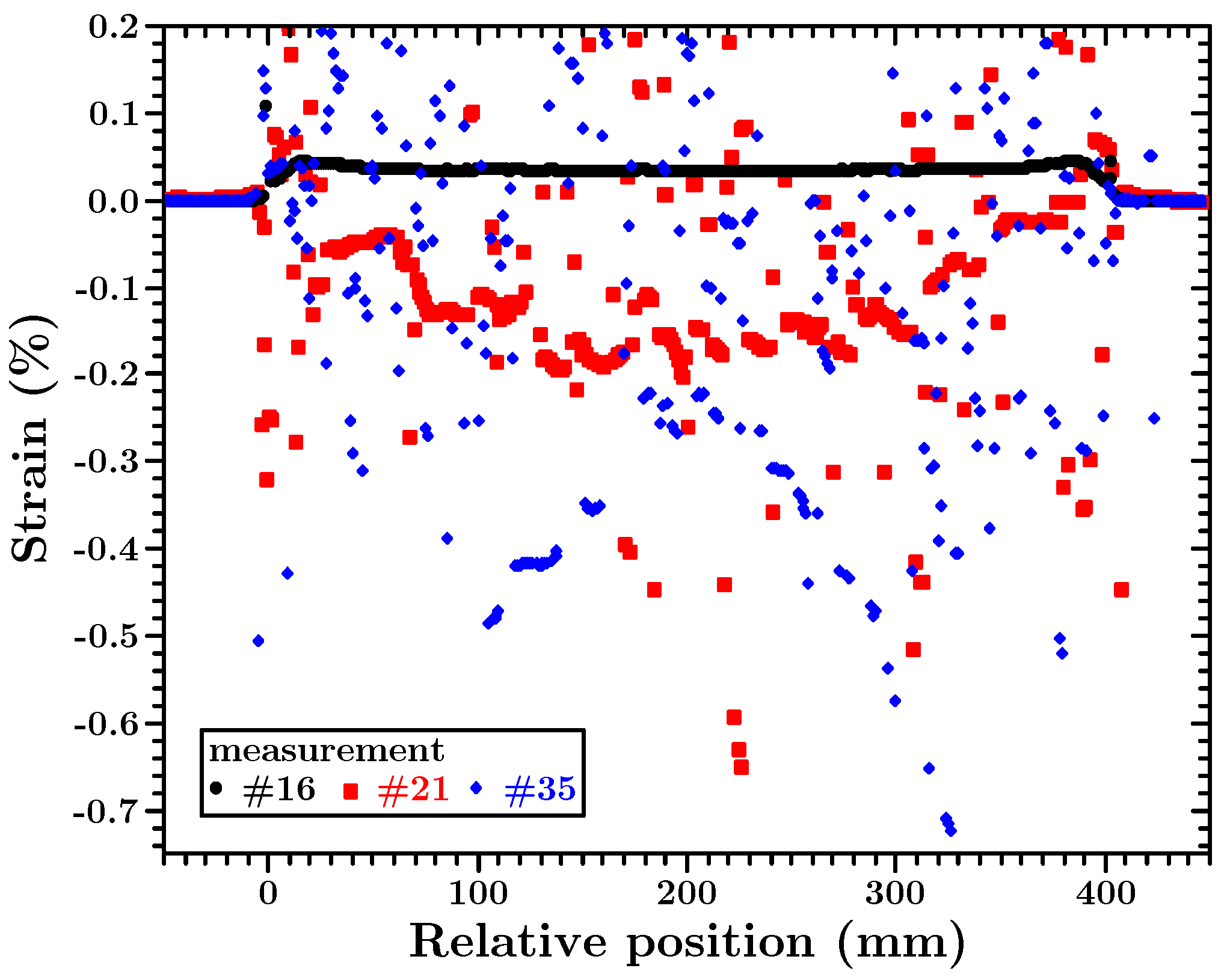
In the following, this method will be called the traditional or classical approach, and the reference used in this traditional technique will be denoted as “absolute reference record”. Strain measurements from the epoxy curing experiments obtained by the traditional data analysis method are shown in Figure 2. The abscissa in this figure shows the position of the strain measurement along the fiber. In this case, the position is also the length of the epoxy block, as shown in Figure 1. The ordinate shows each local strain measurement as a point.

Three strain-measurements (out of 250) are shown, taken at different times during the cure of the epoxy using the traditional analysis method. Whenever strain data are shown, the position along the length of the fiber is from now on related to the entry point of the fiber into the material. The most striking feature of this graph is the fact that the data for later measurements show much scatter: the above-described procedural noise (cf. Section 3).

Measurement 16 (black dots in Figure 2) provides a very reliable curve. At this time, the fiber is still surrounded by liquid epoxy, and it measures basically the increase in temperature due to the exothermal reaction. The increasing temperature manifests itself as (apparent) positive strain readings. This rather experiment-specific feature is described in detail in [17]. It is important however to note that the fiber is not yet subject to a shrinking environment. Hence, no microbending occurs, and the signal is very clear.

When Measurement Number 21 (red squares in Figure 2) was performed, the solidification had been at a stage at which the surrounding material already “gripped” the fiber. Volume shrinkage of the material clearly resulted in a compression of the fiber, leading to negative strain values. Between Measurements 16 and 21, the temperature increases from 63 to 161 degrees Celsius inside the epoxy. Thus, the negative strain is solely caused by the shrinkage of the sample. We refer to [17] regarding details about the temperature development during similar experiments.

However, the measurement curve shows already many outliers. The outliers look like very local and random strain concentrations, which do not make any physical sense for a block of hardening epoxy. This scatter shows clearly that the traditional measurement method starts to fail to determine properly the strain exactly in all points.

Further, Measurement Number 35 (blue diamonds in Figure 2) exhibits data-points that in their majority can just be described as noise. The blue diamonds may form a “banana” shape in the middle of the sample. However, this trend is interrupted by many outliers.

For even later times, the strain signal deteriorates further, and the majority of the measurements show just (procedural) noise.

It is to be noted that these strain values are still below the maximum absolute strain that could be measured with this same instrument in adhesive joints [35]. Thus, the deteriorating signal cannot be attributed to instrument errors or the OBR technique in general. Rather, it must be due to the surrounding conditions in the embedding material.

5.2. Strain Determined by the Running Reference Method

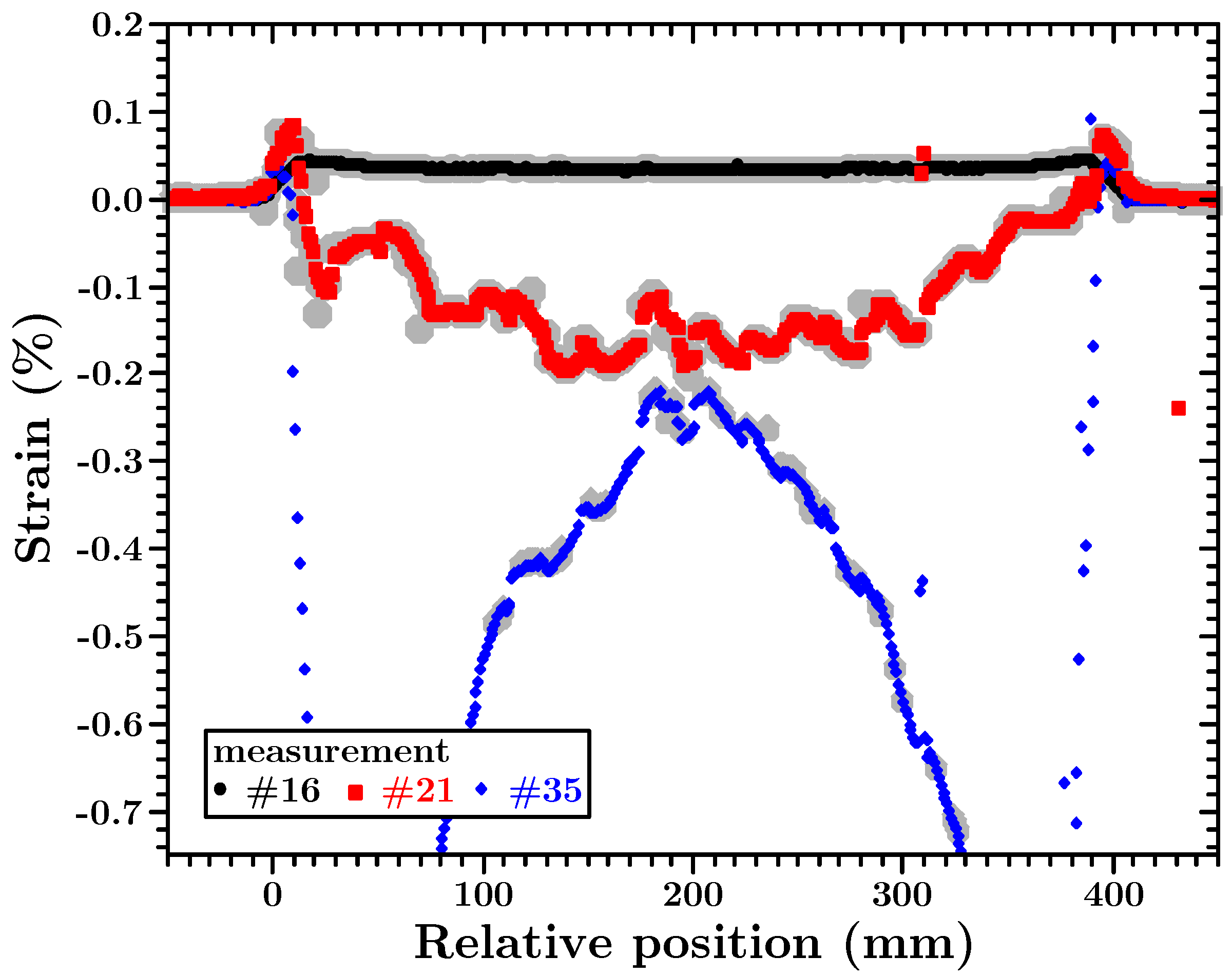
In Figure 3, the strain values can be seen that were retrieved by the running reference method.

The most notable difference between Figure 2 and Figure 3 is the clear measurement curves and that scatter and noise have largely disappeared. To visualize that the proposed new method does indeed lead to the same results as the traditional method, the data shown in Figure 2 are reproduced in Figure 3 as thick grey points in the background.

Even with the rather coarse scale in Figure 3, it can already be seen that both methods yield the same strain values. Of course, a comparison can just take place for the data points in which the absolute reference method yields meaningful results.

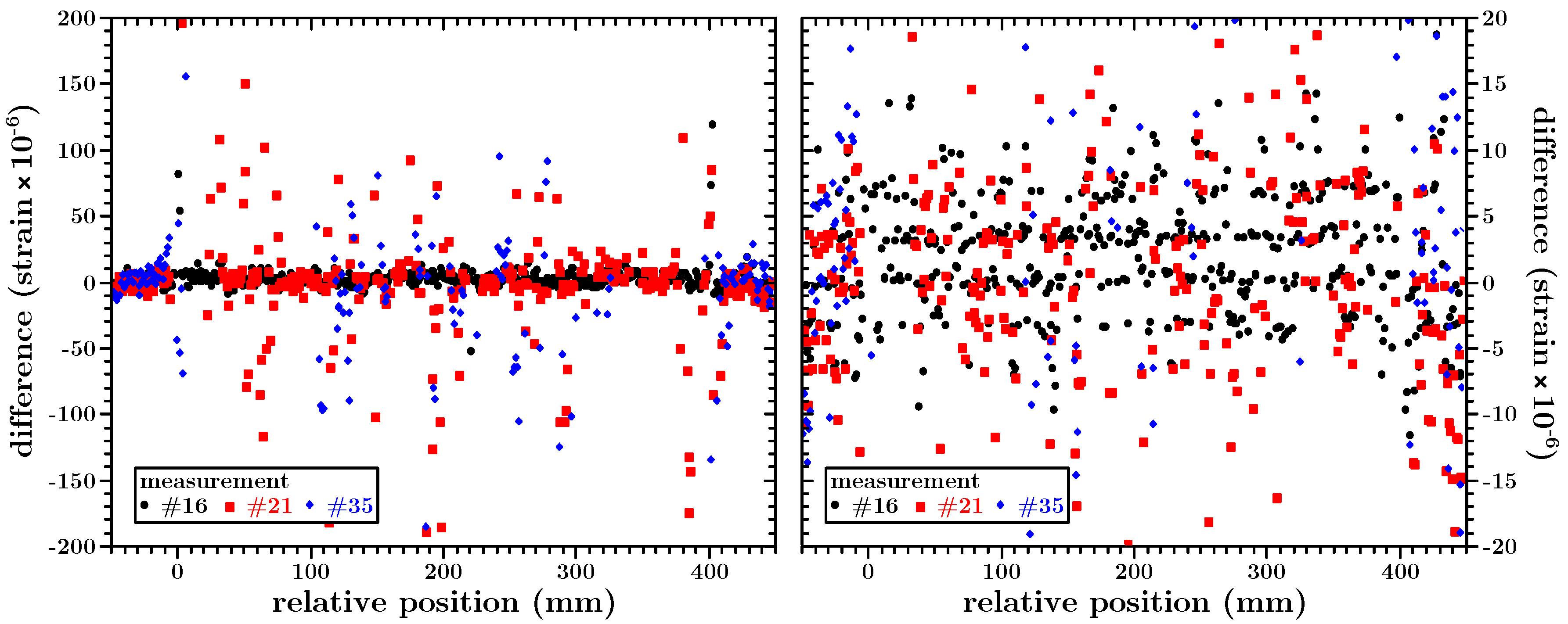
Usually, some kind of Root-Mean-Square Error (RMSE) is given to compare the accuracy of two different methods. However, this is just of very limited applicability for the data presented here, since the traditional method yields mainly noise for later measurements. Only meaningful values could be used, but this would already include a comparison with the strain values determined by the running reference technique. At which threshold of difference a data point is considered to be “correct” is a very subjective, probably hard to justify, interpretation of the data and may amount to “cherry picking” or p-hacking in the worst cases. Hence, to further investigate the accuracy of the running reference method, not the RMSE, but the absolute difference between the strain values obtained by both methods is shown in Figure 4.

The left image in Figure 4 shows that the strain values obtained by both methods are equal within an error range of below 100 ×${10}^{-6}$ strain. When the data points obtained by the traditional method are more reliable (e.g., in the area before the fiber enters the material or for measurements before the epoxy “grips” the fiber), this error can be considered ten-times smaller, as can be seen in the right image in Figure 4. The “bands” in Measurement 16 are due to the maximum resolution of the OBR.

When the traditional method yields noise, the differences in the values obtained by the running reference method exceed by far the herein shown y-scale. This however need not be considered.

It may be noted that for Measurement 16, an RMSE of 5.5 ×${10}^{-6}$ strain is calculated. This is almost the resolution limit for strain values of the instrument used. Ten obvious outliers had to be removed from the data retrieved by the traditional method to calculate the RMSE. These outliers were detected by the algorithm described in the Appendix A. For the other measurements, the above comments are valid. Hence, no such values will be presented here.

These results show that both methods yield the same absolute strain values within an error almost solely defined by the instrument resolution. However, the much lower occurrence of outliers in the data obtained by the running reference method, and thus far more reliable results, shows the superiority of the proposed analysis method compared to the traditional approach.

6. Proof for Backscatter Signal Amplitude Deterioration

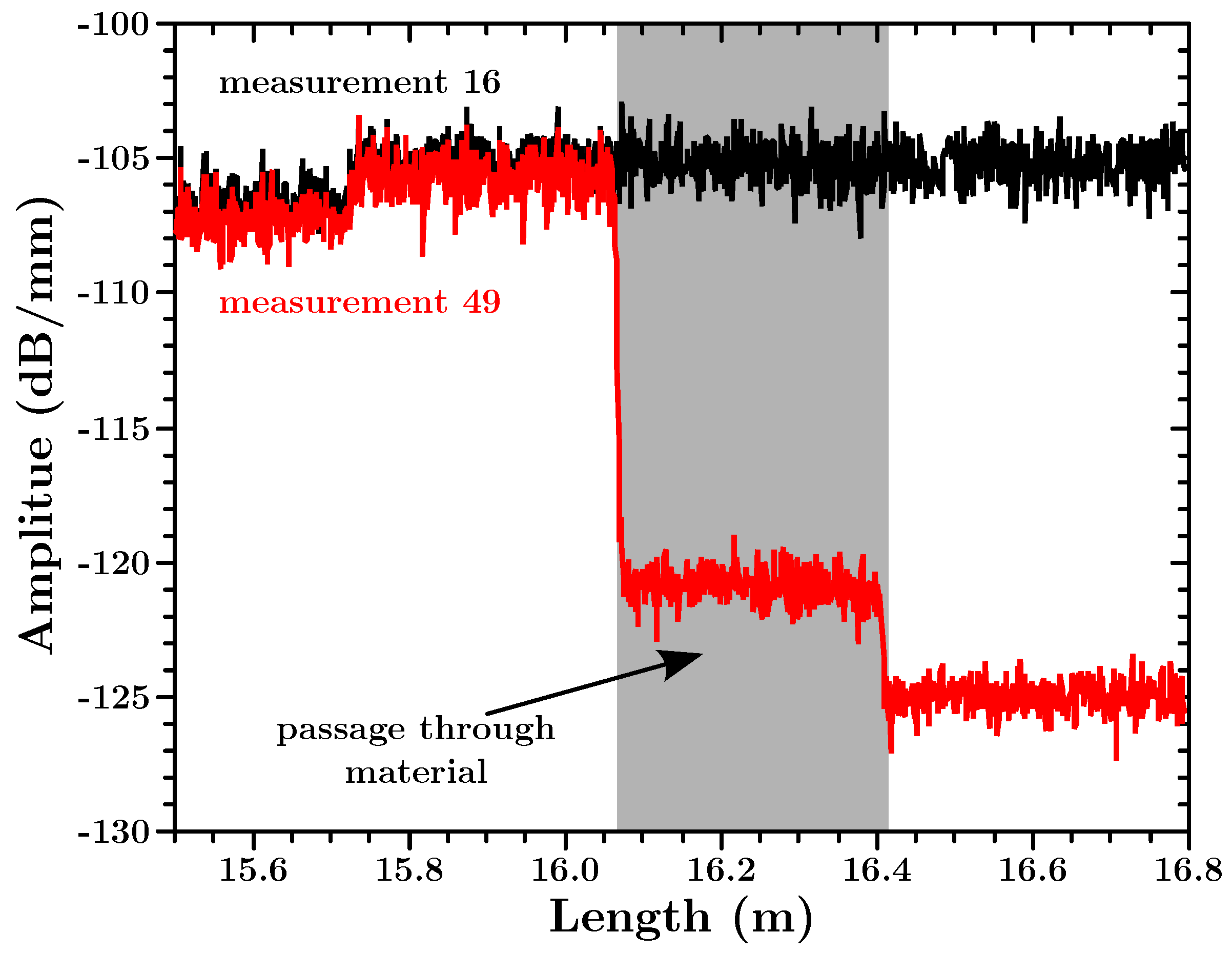
In Section 3, it is described that a hardening and shrinking material can lead to microbending of the fiber. This phenomenon manifests itself in a diminishing backscatter signal amplitude. In turn, strain measurements obtained by the traditional method contain mostly the observed procedural noise. The magnitude of the backscattered signal is shown in Figure 5 as the received amplitude of the signal in dB/mm.

The black curve in Figure 5 shows the backscatter amplitude signal of Measurement 16. As described in Section 5.1, the fiber at this time is still surrounded by liquid epoxy. Thus, it does not experience microbending, and within the borders of natural signal variations the backscatter amplitude signal is a straight line, not exhibiting any signs of a deteriorating amplitude (the step at ca. 15.7 m is due to the splice of the measurement fiber to an extension fiber, which is connected to the OBR instrument). The backscatter amplitude signal for Measurement 49 (red curve in Figure 2), however, shows a step structure, and the amplitude decrease can clearly be attributed to the passage of the fiber through the hardening and shrinking material. Within the material, the amplitude stays constant.

As can be seen in Figure 2, the amplitude diminishes by more than 15 dB/mm, and the signal is only 4 dB/mm from the background signal amplitude. However, as Figure 3 shows, the running reference method is still able to retrieve reliable strain values.

When the backscatter signal becomes undistinguishable from the background signal (e.g., after the fiber exits the material in Figure 5), the comparison of a random background noise record with the (any) reference record leads to the computing of truly random, and not procedural, noise. Since the background signal does not contain any information, not even the running reference analysis method can retrieve reliable strain values.

These results show clearly that curing epoxy indeed treats the fiber so badly that by using the traditional method, no relevant strain data can be obtained any longer, even though the physical limits of the OBR instrument were not reached. How these shortcomings can be overcome without new measurements but by only utilizing the already available data shall be covered in the remainder of this article.

7. Challenges in Connection with the Running Reference Method

The running reference method cannot avoid shot noise, in contrast to the procedural noise of the traditional method. Hence, data retrieved by the running reference method still contain outliers (as defined, e.g., by Grubbs in [52]: “An outlying observation, or ‘outlier’, is one that appears to deviate markedly from other members of the sample in which it occurs.” The sample for which the comparison takes place may be locally defined (cf. Appendix A).). Since the data are added up to get the absolute strain status for each measurement, an outlier in one measurement will be carried through all the subsequent absolute strain values. This can be seen in Figure 3. The two outliers in Measurement Number 21 at a position of ca. 310 mm can also be seen at the same position in Measurement Number 35, but not in Measurement Number 16. In this case, the original outlier was in the data for Measurement Number 18 (not shown). 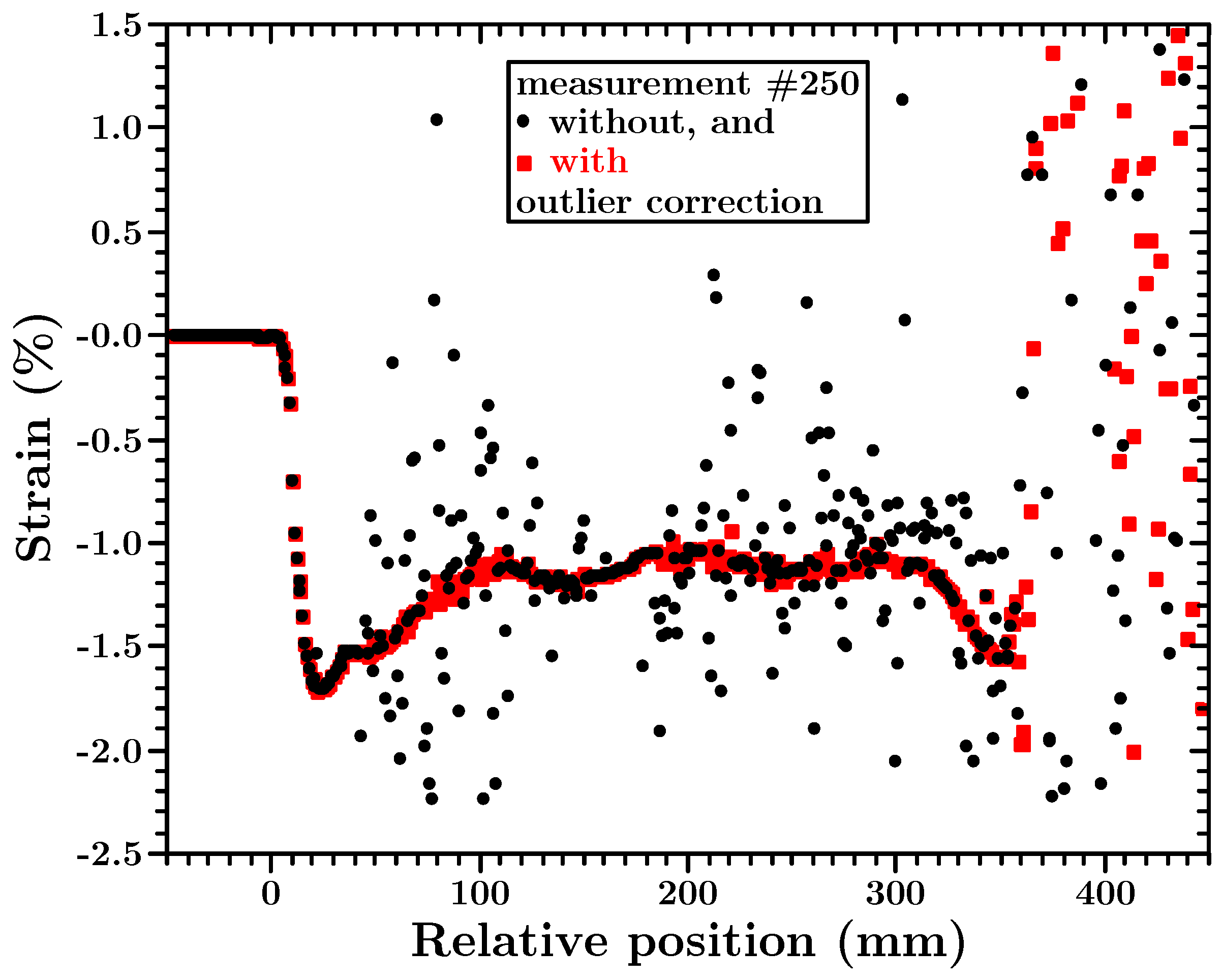To illustrate this issue better, in Figure 6, the absolute strain data obtained by the running reference method for Measurement Number 250 can be seen.

The black dots show the strain values for data retrieved by the running reference method, but not corrected for outliers, while for the red squares each obtained strain; the dataset was corrected for the very few remaining outliers before adding it up. This illustrates the importance of correcting outliers even if the data are retrieved by the running reference approach.

Since data have to be summed up to get the strain values for a certain measurement, an outlier cannot just simply be taken out of the dataset. This would be like using the value zero when adding the data up, which would still lead to an outlier, albeit with a different magnitude. These points rather must be substituted by a reasonable value. It is recommended to always report the data with and without outlier correction. This approach allows others to evaluate the validity of the data correction process.

However, the following is to be said: approximately 40% of the 450 absolute strain values before the fiber leaves the material in Measurement Number 250 can be seen as outliers. However, one has to consider that the running reference method requires evaluating more then 100,000 data points to acquire Measurement Number 250. This means that the possibility for an outlier is far below one percent. Compared to the traditional method, which returns just noise for the majority of all measurements, this can be seen as an improvement. If these comparatively very few outliers are corrected for in the measurement they occur in, the data can be improved, as the red squares in Figure 6 show. The fiber leaves the material around 400 mm. Since the backscatter amplitude drops at that point to the background noise level, it is a physical impossibility to retrieve any information beyond this point (cf. Section 6).

A short summary of such an outlier correction algorithm would be the following. Firstly, search for sections of continuous points that exhibit no strain deviation above a certain, user-defined threshold. This can be regarded as a local minimum/maximum criterion. Secondly, points that exceed the strain threshold are considered outliers. Thirdly, such outliers are replaced by a linear interpolation between the two continuous sections to the left and right of the outlier. Certain measures are taken in order not to dismiss false positives. The interested reader is referred to the Appendix in which a detailed algorithm is presented, which allows the implementation of such outlier detection and correction in simple software. An actual implementation of this algorithm can be found on GitHub [53] under a free software license [54] (see also the location of resources in Section 9).

Some potential users may perceive it as a challenge that the running reference analysis method needs a (semi-)continuous data history to work. The differences in the physical state of the fiber from one measurement to the next must be small enough to not lead to disturbances in the strain data retrieved. This may require taking more measurements than usual. However, this process can be automated, and free software for automated measurements is provided for the reader [53].

The only drawback of the running reference method is the necessity to load not just the new measurement-file, but also the new reference file into the proprietary OBR analysis software that comes with the OBR instrument for each measurement. This considerably increases the work of analyzing the data. However, again, automatization of this task will not require supervision by the user, and free software is provided on GitHub [53] for that purpose.

These are the main challenges that may lead engineers and scientists to perceive the running reference method as too cumbersome to use. However, all four of these issues can easily be overcome by automatizing the involved processes: measuring, data analysis, outlier correction and adding up the strain differences to the absolute strain values.

8. Conclusions

Optical backscatter reflectometry is an easy to use method to obtain information about the strain inside large cast structures during the hardening process of the casting material, like, e.g., cement or a polymer. However, the optical fiber used for these strain measurements may be subject to physical conditions that will not allow obtaining meaningful data with the regular post-processing methods used nowadays.

In this work, an experimental setup is presented to attain such conditions on the optical fiber in epoxy. It is shown that the strain data deteriorate significantly, before the physical limits of the OBR instrument used are reached.

Without the need for new equipment or software, we propose a new way to approach the data analysis to retrieve the strain values. This proposed method determines the strain differences from one measurement to the next instead of the absolute strain compared to before the measurement started. Adding up these strain differences yields the absolute strain for a given measurement.

As long as the traditional method returns meaningful data, it is shown that the new method yields the same strain values. The newly-developed running reference approach, however, works even when the traditional method fails to deliver results.

Four challenging issues of the new approach are discussed and how these can easily be overcome by automatizing the involved steps.

The software used by the authors is provided to the community. It is extensively documented and commented, free of charge and published under the GPL Version 3 [54]. Among other things, this license gives the user the right to change the software according to his/her requirements without the need to ask the authors for allowance. By providing these simple tools under this license, we hope to encourage interested scientists and engineers to apply the running reference analysis method when handling challenging OBR data.

9. Ressources

The OBR raw data, the strain data calculated from the raw data (using the proprietary Luna Instrument software) and the code for the software used in this work are available under [55].

The code for the programs is also published on GitHub [53].

All code is written in Python 2.7.3 and published under the GPL Version 3 [54]. All code is extensively documented to allow for easy user adjustments.