Unsupervised Learning for Concept Detection in Medical Images: A Comparative Analysis


Institute of Electronics and Informatics Engineering of Aveiro, University of Aveiro; Campus Universitário de Santiago, 3810-193 Aveiro, Portugal
*
Author to whom correspondence should be addressed.
Appl. Sci. 2018, 8(8), 1213; https://doi.org/10.3390/app8081213
Submission received: 18 June 2018
/
Revised: 13 July 2018
/
Accepted: 21 July 2018
/
Published: 24 July 2018
(This article belongs to the Special Issue Deep Learning and Big Data in Healthcare)
Abstract
:As digital medical imaging becomes more prevalent and archives increase in size, representation learning exposes an interesting opportunity for enhanced medical decision support systems. On the other hand, medical imaging data is often scarce and short on annotations. In this paper, we present an assessment of unsupervised feature learning approaches for images in biomedical literature which can be applied to automatic biomedical concept detection. Six unsupervised representation learning methods were built, including traditional bags of visual words, autoencoders, and generative adversarial networks. Each model was trained, and their respective feature spaces evaluated using images from the ImageCLEF 2017 concept detection task. The highest mean score of was obtained using representations from an adversarial autoencoder, which increased to when combined with the representations from the sparse denoising autoencoder. We conclude that it is possible to obtain more powerful representations with modern deep learning approaches than with previously popular computer vision methods. The possibility of semi-supervised learning as well as its use in medical information retrieval problems are the next steps to be strongly considered.
1. Introduction
In an era of a steadily increasing use of digital medical imaging, image recognition poses an interesting prospect for novel solutions supporting clinicians and researchers. In particular, the representation learning field has grown fast in recent years [1], and many of the breakthroughs in this field are occurring in deep learning methods which have also been strongly considered in healthcare [2]. Leveraging representation learning tools to the medical imaging field is feasible and worthwhile, as they can provide additional levels of introspection of clinical cases through content-based image retrieval (CBIR).
While multiple initiatives for the provision of medical imaging data sets exist, the process of annotating the data with useful information is exhaustive and requires medical expertise, as it often nails down to a medical diagnosis. In the face of few to no annotations, unsupervised learning stands as a possible means of feature extraction for a measurement of relevance, leading to more powerful information retrieval and decision support solutions in digital medical imaging.
Although unsupervised representation is limited for specific classification tasks when compared to supervised learning approaches, the latter requires an exhaustive process from experts to obtain annotated content. Unsupervised learning, which avoids this issue, can also provide a few other benefits, including transferability to other problems or domains, and can often be bridged to supervised and semi-supervised techniques. We hypothesize that a sufficiently powerful representation of images will enable a medical imaging archive to automatically detect biomedical concepts with some level of certainty and efficiency, thus improving the system’s information retrieval capability over non-annotated data.
In this work, we present an assessment of unsupervised mid-level representation learning approaches for images in the biomedical domain. Representations are built using an ensemble of images from existing biomedical literature. The learned representations were validated with a brief qualitative feature analysis and by training simple classifiers for the purpose of biomedical concept detection. We show that feature learning methods based on deep neural networks can outperform techniques that were previously common-place in image recognition, and that models with adversarial networks, albeit harder to train, can improve the quality of feature learning.
Related Work
Representation learning, or feature learning, can be defined as the process of learning a transformation from a data domain into a representation that makes other machine learning tasks easier to approach [1]. The concept of feature extraction can be employed when this mapping is obtained with handcrafted algorithms rather than learned from the original data in the distribution. Representation learning can be achieved using a wide range of methods, such as k-means clustering, sparse coding [3] and Restricted Boltzmann Machines (RBMs) [4]. In image recognition, algorithms based on bags of visual words have been prevalent, as they have shown superior results over other low-level visual feature extraction techniques [5,6]. More recently, however, image recognition has had a strong focus on deep learning techniques, often with impressive results. Among these, approaches based on autoencoders [7,8] have been considered and are still prevalent to this day.
Research on representation learning has had an intense focus on the ground-breaking concept of generative adversarial networks (GANs) [9]. GANs devise a min-max game in which a generator of “fake” data samples attempts to fool a discriminator network which, in turn, learns to discriminate fake samples from real ones. As the two components mutually improve, the generator will ultimately produce visually-appealing samples that are similar to the original data. The impressive quality of the samples generated by GANs has led the scientific community to devise new GAN variants and applications to this adversarial loss, including for feature learning [10].
Representation learning has been notably used in medical image retrieval, although, even in this decade, handcrafted visual feature extraction algorithms are frequently considered in this context [11,12]. Nonetheless, although the interest in deep learning is relatively recent, a wide variety of neural networks have been studied for medical image analysis [13,14], as they often exhibit greater potential for the task [15]. The use of unsupervised learning techniques is also well regarded as a means of exploiting as much of the available medical imaging data as possible [16].
2. Methods
We considered a set of unsupervised representation learning techniques, both traditional (as in, employing classic computer vision algorithms) and based on deep learning, for the scope of images in the biomedical domain. These representations were subsequently used for the task of biomedical concept detection. Namely,
- We experimented with creating image descriptors using bags of visual words (BoWs), for two different visual keypoint extraction algorithms; and
- With the use of modern deep learning approaches, we designed and trained various deep neural network architectures: a sparse denoising autoencoder (SDAE), a variational autoencoder (VAE), a bidirectional generative adversarial network (BiGAN), and an adversarial autoencoder (AAE).
2.1. Bags of Visual Words
For each data set, images were converted to grayscale without resizing, and visual keypoint descriptors were subsequently extracted. We employed two keypoint extraction algorithms separately: Scale Invariant Feature Transform (SIFT) [17], and Oriented FAST and Rotated BRIEF (ORB) [18]. While both algorithms obtain scale and rotation invariant descriptors, ORB is known to be faster and require less computational resources. The keypoints were extracted and their respective descriptors computed using OpenCV [19] (version 3.3.0, OpenCV team, 2017). Each image yielded a variable number of descriptors of fixed size (128-dimensional for SIFT, 32-dimensional for ORB).
In the event that the algorithm did not retrieve any keypoints for an image, the algorithm’s parameters were adjusted to loosen the edge detection criteria. In SIFT, the contrast threshold (contrastThreshold) was changed from to ; the edge threshold (edgeThreshold) was increased from 10 to 20; and the sigma of the Gaussian on the first octave (sigma) was modified from to . With ORB, the FAST keypoint detection threshold (fastThreshold) was changed from 20 to 10. Nonetheless, such cases of images yielding no keypoints were residual in the data set (less than 0.05% of all images), and occurred mostly in images with little to no potential for visual understanding.
All procedures described henceforth were the same for both ORB and SIFT keypoint descriptors. From the training set, 3000 files were randomly chosen and their respective keypoint descriptors collected to serve as template keypoints. A visual vocabulary (codebook) of size was then obtained by performing k-means clustering on all template keypoint descriptors and retrieving the centroids of each cluster, yielding a list of 512 keypoint descriptors .
Once a visual vocabulary was available, we constructed an image’s BoW by determining the closest visual vocabulary point and incrementing the corresponding position in the BoW for each image keypoint descriptor. In other words, for an image’s BoW , for each image keypoint descriptor , was incremented when the smallest Euclidean distance from to all other visual vocabulary points in V was the distance to . Finally, each BoW was normalized so that all elements lay between 0 and 1. The idea was to picture the bag of visual words as a histogram of visual descriptor occurrences to be used as a global image descriptor [20].
2.2. Deep Representation Learning
Modern representation techniques often rely on deep learning methods. We considered a set of deep convolutional neural network architectures to infer a late feature space over biomedical images. These models were composed of parts with a very similar numbers of layers and parameters in order to obtain a fairer comparison in the evaluation phase. This also meant that the models had very similar resource requirements (time, processing power, and memory) for feature extraction.
Training samples were obtained through the following process: images were resized so that their shorter dimension (width or height) was exactly pixels. Afterwards, the sample was augmented by feeding the networks random crops of size (out of 9 possible kinds of crops: 4 corners, 4 edges and center). Validation images were resized to fit the dimensions. For all cases, the images’ pixel RGB values were normalized to fit in the range [−1, 1]. Unless otherwise mentioned, the networks assumed a rescale size of and a crop size of .
Models with an encoding or discrimination process for visual data were based on the same convolutional neural network architecture, described in Table 1. These models were influenced by the work on deep convolutional generative adversarial networks [21]. Each encoder layer was composed of a 2D convolution, followed by a normalization algorithm and a non-linearity. The specific normalization and activation employed were dependent on the particular model and were concretely indicated in their respective sub-sections. At the top of the network, global average pooling was performed, followed by a fully connected layer, yielding the code tensor z. The Details column in both tables may include the normalization and activation layers that follow a convolution layer, where ReLU stands for the standard, non-leaking rectified linear unit .
The decoding blocks replicate the encoding process in inverse order (Table 2). This starts with a fully connected network from the latent (or prior) code vector and is subsequently transformed through a series of convolutional layers. Transposed convolutions were used in these blocks (also called fractionally-strided convolution in the literature and deconvoluted in a few other papers). The weights of the network were randomly initialized with a Gaussian distribution.
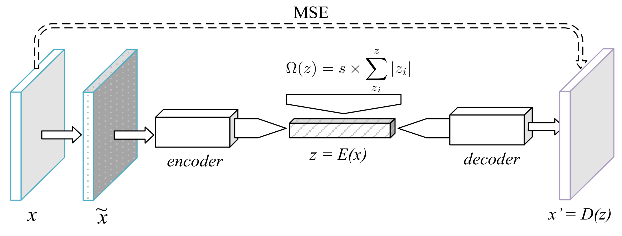
2.2.1. Sparse Denoising Autoencoder
The first tested deep neural network model iwa a common autoencoder with denoising and sparsity constraints (Figure 1). In the training phase, a Gaussian noise with a standard deviation of 0.05 was applied over the input, yielding a noisy sample, . As a denoising autoencoder, its goal was to learn the pair of functions so that was closest to the original input, x. The aim of making E a function of was to force the process to be more stable and robust, thus leading to higher quality representations [7].
Sparsity was achieved with two mechanisms. First, a ReLU activation was used after the last fully connected layer of the encoder, turning negative outputs from the previous layer into zeros. Second, an absolute value penalization was applied to z, thus adding the extra minimization goal of keeping the code sum small in magnitude. The final decoder loss function was therefore
where
is the sparsity penalty function; is the number of pixels in the input images; and x represents the original input without synthesized noise. s is the sparsity coefficient, which we left defined as . This network used batch normalization [22] and standard ReLU activations.
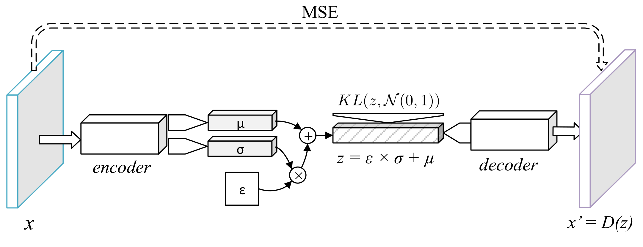
2.2.2. Variational Autoencoder
The encoder of the variational autoencoder (Figure 2) learnt a stochastic distribution which could be sampled from by minimizing the Kulback–Leibler divergence with a unitary normal distribution [8]. The architecture of this network resembled the SDAE with a relevant exception at the encoding process. In order for the encoder to produce a sample distribution, the final dense layer was replaced with two layers of equal dimensions and . The encoded sample was obtained with the reparameterization trick—given , the latent code becomes . The VAE’s loss function was therefore
where and is the Kulback–Leibler divergence from the learned distribution.
Like in the SDAE, convolutional layers were followed by batch normalization [22] and ReLU activations.
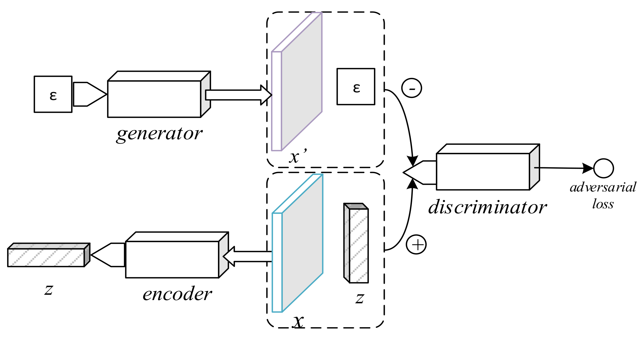
2.2.3. Bidirectional GAN
While GANs are known to show great potential for representation purposes, the basic GAN architecture does not provide a means to encode samples to their respective prior. The bidirectional GAN, depicted in Figure 3, addresses this concern by including an encoder component which learns the inverse process of the generator [10]. Rather than only observing data samples, the BiGAN discriminator’s loss function depends on the code-sample pair. The training process can be formally defined by the following equation:
The encoder component relies on the same convolutional neural network design as the rest, with an exception suggested in reference [10], where the original data was fed to the encoder with a size s of 112 × 112, cropped from images with the shortest dimension resized to 128 pixels (as in, ). Images were still down-sampled to 64 × 64 in order to be fed to the discriminator. The discriminator, in turn, was conceived as follows:
- Like in the encoder, the image was processed by the convolutional neural network described in Table 1 with ;
- The prior code, z, was fed to two fully connected layers with an output shape of B × 64 (where B is the batch size);
- The two outcomes, (1) and (2), were concatenated to form a tensor of shape B × 192, followed by 2 fully connected networks of shape B × 512;
- Finally, a fully connected layer with a single neuron (Bx1) produced the output .
Like in reference [10], all constituent parts of the GAN were optimized simultaneously in each iteration. The encoder and the discriminator of this model used layer normalization [23] and leaky ReLU with a leaking factor of 0.2 on all layers except the discriminator’s last convolutional layer, which is indicated in step (1), and the final output, stated in step (4).
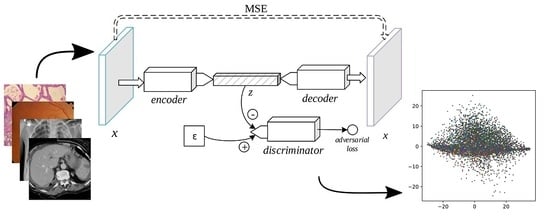
2.2.4. Adversarial Autoencoder
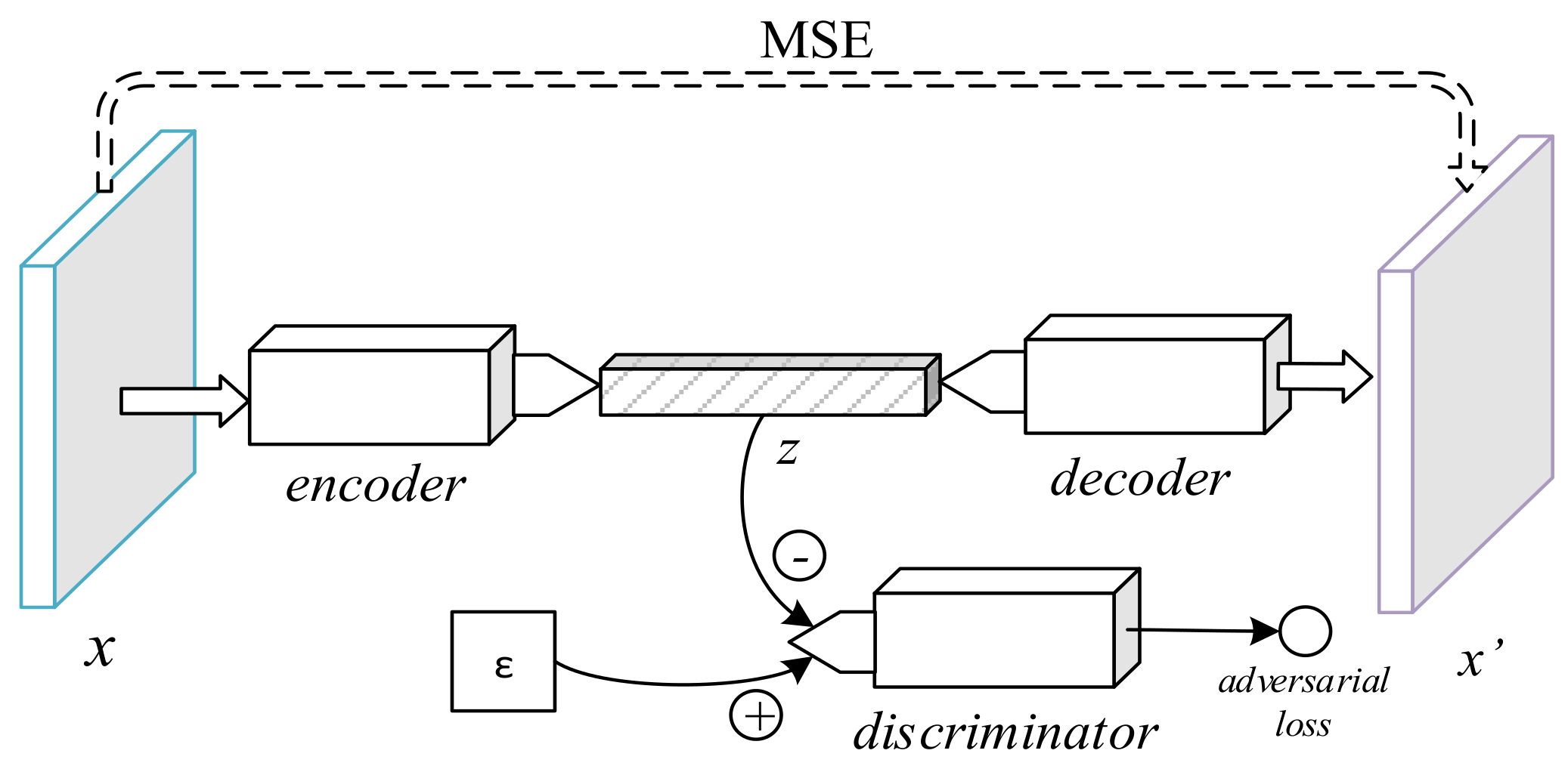
The adversarial autoencoder (AAE), depicted in Figure 4, is an autoencoder in which a discriminator is added to the bottleneck vector [24]. While reducing the -norm distance between a sample and its decoded form (as in the SDAE and the VAE), the AAE includes an adversarial loss to distinguish the encoder’s output from a stochastic prior code, thus serving as a regularizer to the encoding process. The min-max game is thus formally defined as
Our AAE used a simple code discriminator composed of 2 fully connected layers of 128 units with leaky ReLU activation for the first two layers, followed by a single neuron without a non-linearity. During training, the discriminator was fed a prior z sampled from a random normal distribution as the real code, and the output of the encoder as the fake code. The model used layer normalization [23] on all except the last layers of each component and leaky ReLU with a leaking factor of 0.2. Like in reference [10], all three components’ parameters were updated simultaneously in each iteration.
2.2.5. Network Training Details
The networks were trained through stochastic gradient descent, using the Adam optimizer [25]. The hyperparameter was set to 0.5 for the BiGAN and AAE, and 0.9 for the remaining networks.
Each neural network model was trained over 206,000 steps, which is approximately 100 epochs, with a mini-batch size of 64. The base learning rate was 0.0005. The learning rate was multiplied by 0.2 halfway through the training process (50 epochs) to facilitate convergence.
All neural network training and latent code extraction was conducted using TensorFlow, and TensorBoard was used during the development for monitoring and visualization [26]. Depending on the particular model, training took, on average, 120 h (a maximum of 215 h, for the adversarial autoencoder) to complete on one of the GPUs of an NVIDIA Tesla K80 graphics card in an Ubuntu server machine.
2.3. Evaluation
The previously described methods for representation learning were aimed towards addressing the domain of biomedical images. A proper validation of these features was made with the use of the data sets from the ImageCLEF 2017 caption challenge [27], specifically the portion corresponding to the concept detection task. In 2017, the focus of the ImageCLEF Caption challenge was on automated medical image understanding for quicker decision-making in clinical diagnoses. As the first sub-task of the caption prediction challenge, the goal of the concept detection task was to conceive a computer model to identify the individual concepts from medical images, from which full captions could be composed.
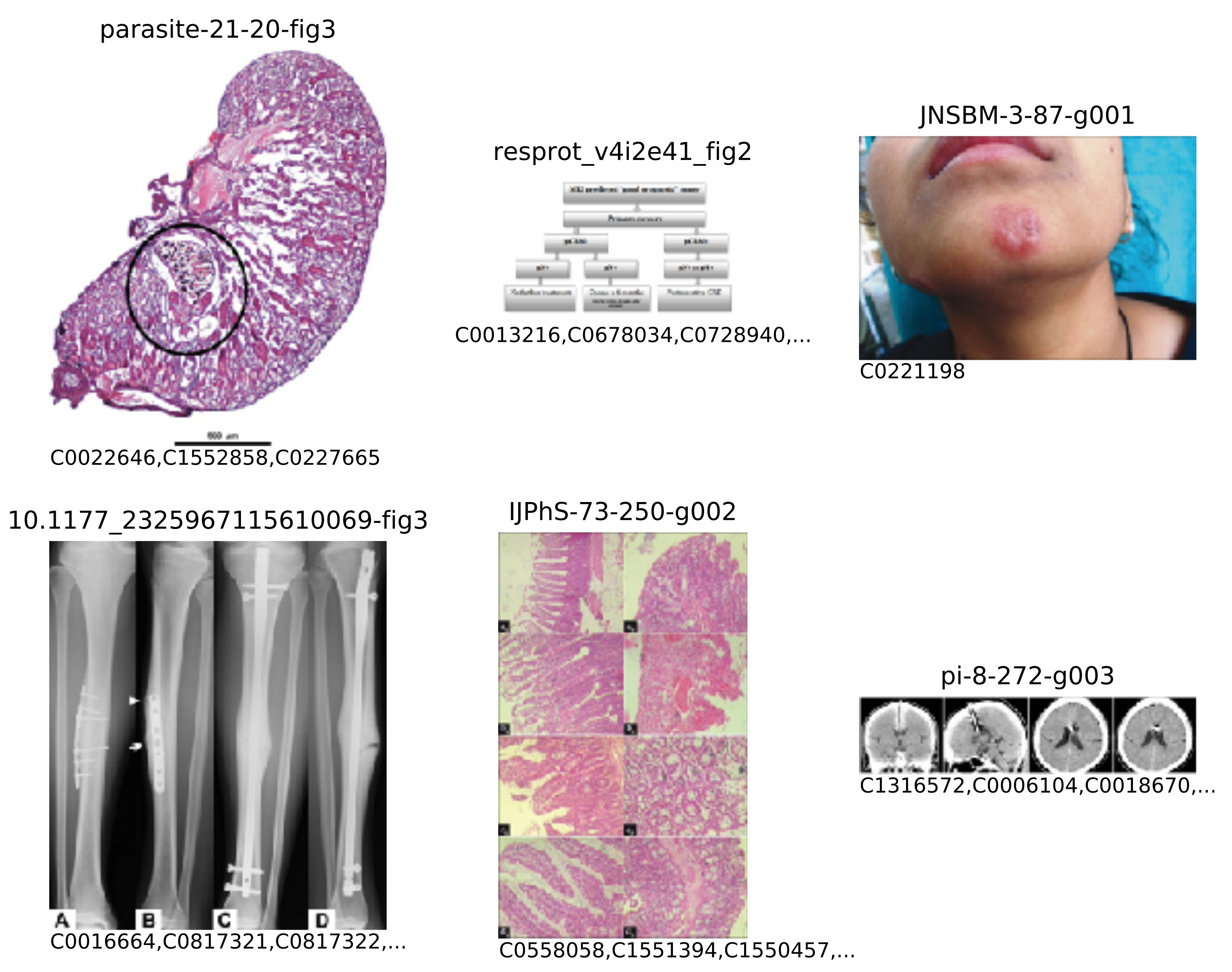
This task was accompanied by a collection of images, originally seen in open access biomedical journals from the PubMed Central and encompassing a wide variety of modalities (radiology, biopsy, pathology, and general diagrams, to name a few). Images were formatted in JPEG, with resolutions varying from 400 to 800 pixels in either dimension. Each image was also accompanied by its respective caption (which was not used in this work), along with the extracted list of biomedical concepts. The concepts were written as concept unique identifiers (CUIs) from the Unified Medical Language System (UMLS (https://www.nlm.nih.gov/research/umls)). A few examples from the collection are shown in Figure 5, and small insights into the concepts present in these images may be obtained from Table 3. The full data set was divided into three parts: the training set (164,614 images), the validation set (10,000 images), and the testing set (10,000 images). The testing set’s ground truth was hidden during the challenge but was provided to the participants later on.
Each of the set of features, learned from the approaches described in the previous section, were used to train simple classifiers for concept detection. In both cases, the same training and validation folds from the original data set were considered, after being mapped to their respective feature spaces. In addition, data points in the validation set with an empty list of concepts were discarded.
These simple models were used to predict the concept list of each image by sole observation of their respective feature set. Therefore, the assessment of our representation learning methods is made based on the representation’s descriptiveness without learning additional complex feature spaces, and so, on the effectiveness of capturing high-level features from latent codes alone.
2.3.1. Logistic Regression
Aiming for low complexity and classification speed, we performed a logistic regression with stochastic gradient descent for concept detection, treating the UMLS terms as labels. More specifically, linear classifiers were trained over the features, one for each of the 750 (seven-hundred and fifty) most frequently occurring concepts in the training set. All models were trained using follow-the-regularized-leader (FTRL)-Proximal optimization [28] with a base learning rate of , an -norm regularization factor of , and a batch size of 128. Since biomedical concepts are very sparse and imbalanced, the score was considered to be the main evaluation metric, which was calculated with respect to multiple fixed operating point thresholds, (namely , , , , , , , and ), for each sample, and averaged across the 750 labels. The threshold which resulted in the highest mean score on the validation set was recorded, and the respective precision, recall, and area under the ROC curve were also included. Subsequently, the same model and threshold were used to predict the concepts in the testing set, the score of which was retrieved with the official evaluation tool from the ImageCLEF challenge.
Since it is also possible to combine multiple representations with simple vector concatenation, we experimented with training these classifiers using a mixture of features from the SDAE and AAE latent codes. This process is often called early fusion and is contrasted with late fusion, which involves merging the results of separate models. Each model undertook a few dozens of training epochs until the best score among the thresholds would no longer improve. In practice, the training and evaluation of the linear classifiers was done with TensorFlow.
2.3.2. k-Nearest Neighbors
A relevant focus of interest in representation learning is its potential in information retrieval. While concept detection is not a retrieval problem, and the use of retrieval techniques is a naive approach to classification, it is fast and scales better in the face of multiple classes. Furthermore, it enables a rough assessment of whether the representation would fare well in retrieval tasks where similarity metrics have not previously been learned, which is the case for the Euclidean distance between features.
A modified form of the k-nearest neighbors algorithm was used as a second means of evaluation. Each data point in the validation set had its concepts predicted by retrieving the n closest points from the training feature set (henceforth called neighbors) in the Euclidean space and accumulating all concepts of those neighbors into a Boolean sum of labels. This tweak makes the algorithm more sensitive to very sparse classification labels, such as those found in the biomedical concept detection task. All natural numbers from 1 to 5 were tested for the possible k number of neighbors to consider. Analogous to the logistic regression above, the k which resulted in the highest score on the validation set was regarded as the optimal parameter, and predictions over the testing set were evaluated using the optimal k.
The actual search for the nearest neighbors was performed using the Faiss library which contributed to rapid retrieval [29]. Feature fusion was not considered in the results, as they did not seem to bring any improvement over singular representations.
3. Results
3.1. Qualitative Results
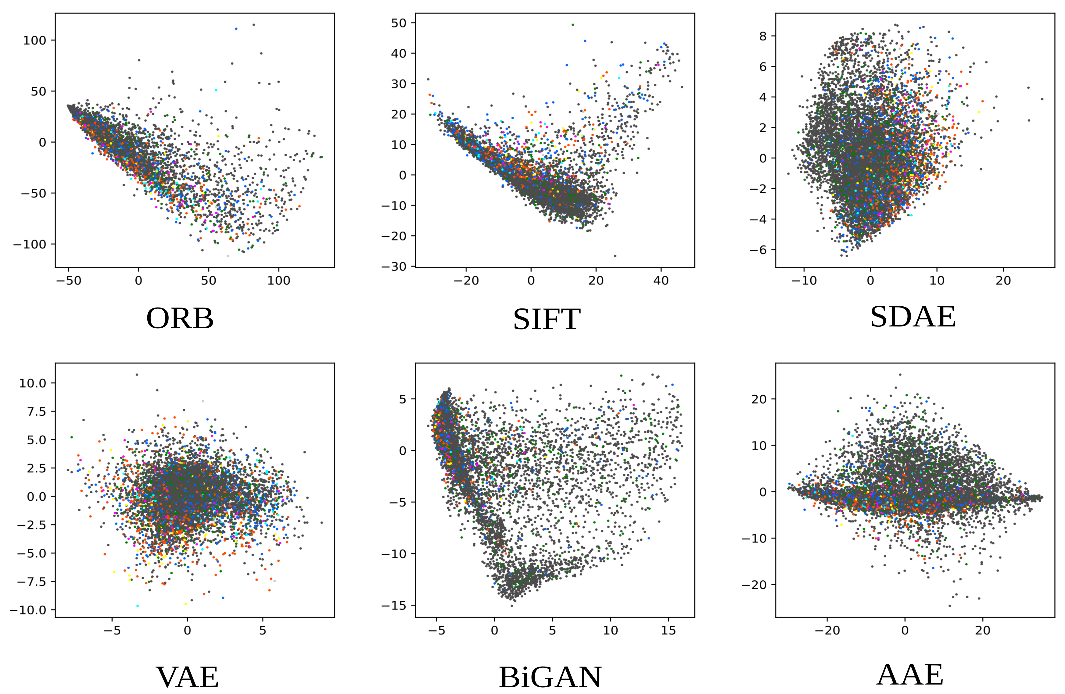
Each representation learning approach described in this work resulted in a 512-dimensional feature space. Figure 6 shows the results of mapping the validation feature set of each representation learned into a two-dimensional space using principal component analysis (PCA). The three primary colors were used (red, green, and blue) to label the points with the three most commonly occurring UMLS terms in the training set, namely C1696103 (image-dosage form), C0040405 (X-ray CT), and C0221198 (lesion), each painted in an additive fashion.
While extreme outliers were removed from the figures, it can be noted that the ORB, SIFT and BiGAN representations had more outliers than the other three representations. A good representation would enable samples to be linearly separable based on their list of concepts. Even though the concept detection task is too hard to allow clear cut separation, one can still identify regions in the manifold in which points of one of the frequent labels are mostly gathered. The existence of concentrations of random points in certain parts of the manifold, as further observed from the classification results, was noticeable mostly in poorer quality representations.
The latent space regularization in representations based on deep learning was also apparent in these plots: both the AAE (with the approximate Jensen–Shannon divergence from the adversarial loss) and the VAE (with the Kullback–Leibler divergence) manifested great similarity with a normal distribution.
3.2. Linear Classifiers
Table 4 shows the best resulting metrics obtained with logistic regression on the validation set, followed by the final score on the testing set. Mix is the identifier given for the feature combination of SDAE and AAE. We observed that, for all classifiers, the threshold of 0.075 yielded the best score. This metric, when obtained with the validation set, assumes the existence of only the 750 most frequent concepts in the training set. Nonetheless, these metrics are deemed acceptable for quantitative comparison among the trained representations and did, indeed, establish the same score ordering as the metrics in the testing set. The adversarial autoencoder obtained the best mean score in concept detection, only superseded by a combination of the same features with those from the sparse denoising autoencoder.
These metrics, although seemingly low, were within the expected range of scores in the domain of concept detection in biomedical images, since the classified labels were very scarce. As an example, only 10.9% of the training set was positive for the most frequent term. For the second and third most frequent terms, the numbers were 9.8% and 8.6%, respectively. The mean number of positive labels of each of the 750 most frequent concepts was 876.7, with a minimum of 203 positive labels for the 750th most frequent concept in the training set. We found that most concepts in the set did not have enough images with a positive label for a valuable classifier.
The scores obtained here can be compared with the results from the ImageCLEF 2017 challenge. The best scores on the testing set, without the use of external resources that could severely bias the results, were 0.1583 and 0.1436 [27]. In the former, the participants performed multi-label classification directly over the images using a neural network model that was pre-trained with the ImageNet and COCO data sets [30]. The use of additional information outside of the given data sets is known to significantly improve the results. In the list of submissions where no external resources were used, these techniques were only outperformed by the submissions from the IPL team [31] which extracted global image descriptors using dense SIFT bags of words and quad-tree bags of colors. While recognizing the fact that the work also relied on building global features in an unsupervised manner, the representations obtained in our work were significantly more compact in size and thus, more computationally efficient in practice.
The combined representation of concatenating the feature spaces of the SDAE and AAE resulted in even better classifiers. Although the results of the combined representation are shown here, this improvement is not to be overstated, given that it relies on a wider feature vector and on training two representations that were meant to perform individually. Another relevant observation is that the representations based on BoWs were generally less effective for the task than deep representation learning methods. Although SIFT BoWs resulted in a slightly better area under the ROC curve, the chosen operating points led to ORB slightly outperforming SIFT.
It is understood that the thresholds can be better fine-tuned to further increase these numbers [32]. Rather than performing a methodical determination of the optimal threshold, we chose to avoid overfitting the validation set by selecting a few thresholds within the interval known to contain the optimal threshold.
3.3. k-Nearest Neighbors
The results of classifying the validation set with similarity search are presented in Table 5. The presence of lower scores than those with linear classifiers is to be expected. The linear classifier can be interpreted as a model which learns a custom distance metric for each label, whereas k-NN relies on a fixed Euclidean distance metric. With k-nearest neighbors, the best mean score of 0.0751 was obtained with the SDAE. The AAE followed with a mean score of 0.0691. The form of passive fitting over the validation set from the choice of k was much less greedy than the training process of the logistic regression which included a choice of operating threshold and halting condition based on the outcome from the validation set. Therefore, it was expected that the final scores on the testing set would not deviate as much from the scores obtained on the validation set.
4. Conclusions
This paper took unsupervised representation learning techniques from state-of-the-art methods, facing them against a more traditional bags of visual words approach. The methods were evaluated with the biomedical concept detection sub-task of the ImageCLEF 2017 caption prediction task. We tested the hypothesis that a powerful image descriptor can contribute to efficient concept detection with some level of certainty, without observing the original image. Results were presented for six different approaches, where two of them relied on visual keypoint extraction and description algorithms and the other two of them were based on generative adversarial networks. Overall, these methods significantly outperformed our previous participation and were comparable with other techniques in the challenge.
As identified in previous work [33] and hereby ensured, it is possible to obtain more powerful representations with modern deep learning approaches, in contrast with previously popular computer vision methods, such as the SIFT bags of visual words.
Deep neural networks are known to be computationally intensive to train, but recent breakthroughs and open technologies have made these methods more accessible and practical. The convergence of an auto-encoder is relatively easy to attain, as the reconstruction loss constitutes a single major objective that can be optimized to a plateau. This is not the case for GANs, the nature of which imposes two adversarial objectives, thus bringing additional concerns for training stability. In particular, the results obtained with the BiGAN suggest that the model would benefit from better training. GANs can empirically provide good results, but the additional complexity, the difficulty of convergence, and the possibility of mode collapse can significantly cripple their performance in representation learning. Nonetheless, these issues are already a high focus of attention at this time and will likely lead to substantial improvements in GAN design and training.
It is also important that these approaches are augmented with non-visual information. In particular, a medical imaging archive should take advantage of the available data beyond pixel data. Future work will consider semi-supervised learning as a means of building more descriptive representations from known categories and other annotations. Subsequently, these representations are to be evaluated in a medical information retrieval scenario as well as with other data sets in the medical imaging domain.
Author Contributions
Conceptualization, E.P.; Data curation, E.P.; Investigation, E.P.; Methodology, E.P.; Software, E.P.; Supervision, C.C.; Validation, E.P.; Visualization, E.P.; Writing—original draft, E.P.; Writing—review & editing, C.C.
Funding
This work was financed by the ERDF (European Regional Development Fund) through the Operational Programme for Competitiveness and Internationalisation-COMPETE 2020 Programme, and by National Funds through the FCT—Fundação para a Ciência e a Tecnologia, within project PTDC/EEI-ESS/6815/2014. Eduardo Pinho is funded by the FCT under the grant PD/BD/105806/2014.
Conflicts of Interest
The authors declare no conflict of interest.
Abbreviations
The following abbreviations are used in this manuscript:
| CBIR | Content-based Image Retrieval |
| RBM | Restricted Boltzmann Machine |
| GAN | Generative Adversarial Network |
| BoW | Bag of Words |
| SDAE | Sparse Denoising Autoencoder |
| VAE | Variational Autoencoder |
| BiGAN | Bidirectional Generative Adversarial Network |
| AAE | Adversarial Autoencoder |
| SIFT | Scale Invariant Feature Transform |
| ORB | Oriented FAST and Rotated BRIEF |
| ReLU | Rectified Linear Unit |
| CUI | Concept Unique Identifier |
| UMLS | Unified Medical Language System |
| PCA | Principal Component Analysis |
| FTRL | follow-the-regularized-leader |
References
- Bengio, Y.; Courville, A.; Vincent, P. Representation learning: A review and new perspectives. Pattern Anal. Mach. Intell. IEEE Trans. 2013, 35, 1798–1828. [Google Scholar] [CrossRef] [PubMed]
- Ravi, D.; Wong, C.; Deligianni, F.; Berthelot, M.; Andreu-Perez, J.; Lo, B.; Yang, G.Z. Deep Learning for Health Informatics. IEEE J. Biomed. Health Inform. 2017, 21, 4–21. [Google Scholar] [CrossRef] [PubMed]
- Lee, H.; Battle, A.; Raina, R.; Ng, A.Y. Efficient sparse coding algorithms. Adv. Neural Inf. Process. Syst. 2006, 19, 801–808. [Google Scholar]
- Hinton, G.E.; Osindero, S.; Teh, Y.W. A fast learning algorithm for deep belief nets. Neural Comput. 2006, 18, 1527–1554. [Google Scholar] [CrossRef] [PubMed]
- Wangming, X.; Jin, W.; Xinhai, L.; Lei, Z.; Gang, S. Application of Image SIFT Features to the Context of CBIR. In Proceedings of the 2008 International Conference on Computer Science and Software Engineering, Wuhan, China, 12–14 December 2008; pp. 552–555. [Google Scholar] [CrossRef]
- Dimitrovski, I.; Kocev, D.; Kitanovski, I.; Loskovska, S.; Džeroski, S. Improved medical image modality classification using a combination of visual and textual features. Comput. Med. Imaging Graph. 2015, 39, 14–26. [Google Scholar] [CrossRef] [PubMed]
- Vincent, P.; Larochelle, H.; Lajoie, I.; Bengio, Y.; Manzagol, P.A. Stacked Denoising Autoencoders: Learning Useful Representations in a Deep Network with a Local Denoising Criterion. J. Mach. Learn. Res. 2010, 11, 3371–3408. [Google Scholar]
- Kingma, D.P.; Welling, M. Auto-Encoding Variational Bayes. arXiv, 2014; arXiv:1312.6114. [Google Scholar]
- Goodfellow, I.J.; Pouget-abadie, J.; Mirza, M.; Xu, B.; Warde-farley, D.; Ozair, S.; Courville, A.; Bengio, Y. Generative Adversarial Nets. arXiv, 2014; arXiv:1406.2661v1. [Google Scholar]
- Donahue, J.; Krähenbühl, P.; Darrell, T. Adversarial feature learning. arXiv, 2016; arXiv:1605.09782. [Google Scholar]
- Li, Z.; Zhang, X.; Müller, H.; Zhang, S. Large-scale Retrieval for Medical Image Analytics: A Comprehensive Review. Med. Image Anal. 2017. [Google Scholar] [CrossRef] [PubMed]
- Kalpathy-Cramer, J.; de Herrera, A.G.S.; Demner-Fushman, D.; Antani, S.; Bedrick, S.; Müller, H. Evaluating performance of biomedical image retrieval systems—An overview of the medical image retrieval task at ImageCLEF 2004–2013. Comput. Med. Imaging Graph. 2015, 39, 55–61. [Google Scholar] [CrossRef] [PubMed] [Green Version]
- Litjens, G.; Kooi, T.; Bejnordi, B.E.; Setio, A.A.A.; Ciompi, F.; Ghafoorian, M.; van der Laak, J.A.; van Ginneken, B.; Sánchez, C.I. A survey on deep learning in medical image analysis. Med. Image Anal. 2017, 42, 60–88. [Google Scholar] [CrossRef] [PubMed] [Green Version]
- Jimenez-del Toro, O.; Otálora, S.; Andersson, M.; Eurén, K.; Hedlund, M.; Rousson, M.; Müller, H.; Atzori, M. Analysis of histopathology images: From traditional machine learning to deep learning. In Biomedical Texture Analysis; Elsevier: New York, NY, USA, 2018; pp. 281–314. [Google Scholar]
- Sun, W.; Zheng, B.; Qian, W. Automatic feature learning using multichannel ROI based on deep structured algorithms for computerized lung cancer diagnosis. Comput. Biol. Med. 2017, 89, 530–539. [Google Scholar] [CrossRef] [PubMed]
- Wu, G.; Kim, M.; Wang, Q.; Munsell, B.C.; Shen, D. Scalable High-Performance Image Registration Framework by Unsupervised Deep Feature Representations Learning. IEEE Trans. Biomed. Eng. 2016, 63, 1505–1516. [Google Scholar] [CrossRef] [PubMed]
- Lowe, D.G. Distinctive Image Features from Scale-Invariant Keypoints. Int. J. Comput. Vis. 2004, 60, 91–110. [Google Scholar] [CrossRef] [Green Version]
- Rublee, E.; Rabaud, V.; Konolige, K.; Bradski, G. ORB: An efficient alternative to SIFT or SURF. In Proceedings of the 2011 International Conference on Computer Vision, Barcelona, Spain, 6–13 November 2011; pp. 2564–2571. [Google Scholar]
- Bradski, G. The OpenCV Library. Dr. Dobbs J. 2000, 25, 120–126. [Google Scholar]
- Sivic, J.; Zisserman, A. Video Google: A text retrieval approach to object matching in videos. In Proceedings of the Ninth IEEE International Conference on Computer Vision, Nice, France, 13–16 October 2003; pp. 1470–1477. [Google Scholar]
- Radford, A.; Metz, L.; Chintala, S. Unsupervised Representation Learning with Deep Convolutional Generative Adversarial Networks. arXiv, 2016; arXiv:1511.06434. [Google Scholar]
- Ioffe, S.; Szegedy, C. Batch Normalization: Accelerating Deep Network Training by Reducing Internal Covariate Shift. arXiv, 2015; arXiv:1502.03167. [Google Scholar]
- Ba, J.L.; Kiros, J.R.; Hinton, G.E. Layer Normalization. arXiv 2016, arXiv:1607.06450. [Google Scholar]
- Makhzani, A.; Shlens, J.; Jaitly, N.; Goodfellow, I.; Frey, B. Adversarial Autoencoders. arXiv, 2015; arXiv:1511.05644. [Google Scholar]
- Kingma, D.P.; Ba, J.L. Adam: A Method for Stochastic Optimization. arXiv, 2015; arXiv:1412.6980. [Google Scholar]
- Abadi, M.; Agarwal, A.; Barham, P.; Brevdo, E.; Chen, Z.; Citro, C.; Corrado, G.S.; Davis, A.; Dean, J.; Devin, M.; et al. TensorFlow: Large-Scale Machine Learning on Heterogeneous Distributed Systems. arXiv, 2016; arXiv:1603.04467. [Google Scholar]
- Eickhoff, C.; Schwall, I.; de Herrera, A.; Müller, H. Overview of ImageCLEFcaption 2017—The Image Caption Prediction and Concept Extraction Tasks to Understand Biomedical Images; Working Notes CLEF; CEUR-WS.org: Aachen, Germany, 2017. [Google Scholar]
- McMahan, H.B.; Holt, G.; Sculley, D.; Young, M.; Ebner, D.; Grady, J.; Nie, L.; Phillips, T.; Davydov, E.; Golovin, D.; et al. Ad click prediction: A view from the trenches. In Proceedings of the 19th ACM SIGKDD International Conference on Knowledge Discovery and Data Mining, Chicago, IL, USA, 11–14 August 2013; pp. 1222–1230. [Google Scholar]
- Johnson, J.; Douze, M.; Jégou, H. Billion-scale similarity search with GPUs. arXiv, 2017; arXiv:1702.08734. [Google Scholar]
- Dimitris, K.; Ergina, K. Concept Detection on Medical Images Using Deep Residual Learning Network; Working Notes CLEF; CEUR-WS.org: Aachen, Germany, 2017. [Google Scholar]
- Valavanis, L.; Stathopoulos, S. IPL at ImageCLEF 2017 Concept Detection Task; Working Notes CLEF; CEUR-WS.org: Aachen, Germany, 2017. [Google Scholar]
- Lipton, Z.C.; Elkan, C.; Narayanaswamy, B. Thresholding Classifiers to Maximize F1 Score. Mach. Learn. Knowl. Discov. Databases 2014, 8725, 225–239. [Google Scholar] [PubMed]
- Pinho, E.; Silva, J.F.; Silva, J.M.; Costa, C. Towards Representation Learning for Biomedical Concept Detection in Medical Images: UA. PT Bioinformatics in ImageCLEF 2017; Working Notes CLEF; CEUR-WS.org: Aachen, Germany, 2017. [Google Scholar]
Figure 1.
Diagram of the sparse denoising autoencoder.

Figure 2.
Diagram of the variational autoencoder.

Figure 3.
Diagram of the bidirectional generative adversarial network (GAN).

Figure 4.
Diagram of the adversarial autoencoder.

Figure 5.
A few samples from the ImageCLEF 2017 concept detection data set with their respective file IDs and trimmed list of concept identifiers.
Figure 5.
A few samples from the ImageCLEF 2017 concept detection data set with their respective file IDs and trimmed list of concept identifiers.

Figure 6.
The 2D projections of the latent codes in the validation set, for each learned feature space. Best seen in color.
Figure 6.
The 2D projections of the latent codes in the validation set, for each learned feature space. Best seen in color.


Table 1.
A tabular representation of the SimpleNet layers’ specifications.
| Layer | Kernels | Size/Stride | Details |
|---|---|---|---|
| conv1 | 64 | 5 × 5/2 | Normalization + non-linearity |
| conv2 | 128 | 5 × 5/2 | Normalization + non-linearity |
| conv3 | 256 | 5 × 5/2 | Normalization + non-linearity |
| conv4 | 512 | 5 × 5/2 | Normalization + non-linearity |
| conv5 | 512 | 5 × 5/2 | Normalization + non-linearity |
| avgpool | N/A | N/A | |
| fc | nb | Linear activation |
Table 2.
A tabular representation of the decoder/generator layers’ specifications.
| Layer | Kernels | Size/Stride | Details |
|---|---|---|---|
| fc | 4096 | Reshaped to 1024 × 2 × 2 | |
| dconv5 | 512 | 5 × 5/2 | Normalization + ReLU |
| dconv4 | 256 | 5 × 5/2 | Normalization + ReLU |
| dconv3 | 128 | 5 × 5/2 | Normalization + ReLU |
| dconv2 | 64 | 5 × 5/2 | Normalization + ReLU |
| dconv1 | 3 | 5 × 5/2 | Linear activation |
Table 3.
The ten most frequently occurring concepts in the ImageCLEF 2017 training set for concept detection.
Table 3.
The ten most frequently occurring concepts in the ImageCLEF 2017 training set for concept detection.
| CUI | Occurrences in Training Set | Textual Description |
|---|---|---|
| C1696103 | 17998 | Image-dosage form |
| C0040405 | 16217 | X-ray computed tomography |
| C0221198 | 14219 | Lesion |
| C1306645 | 10926 | Plain X-ray |
| C0577559 | 9769 | Mass (lump, localized mass) |
| C0027651 | 9570 | Tumor |
| C0441633 | 9289 | Diagnostic scanning |
| C0817096 | 5602 | Thorax |
| C1317574 | 5039 | Note |
| C0087111 | 4983 | Therapy |
Table 4.
The best metrics obtained from logistic regression for each representation learned, where Mix is the feature combination of sparse denoising autoencoder (SDAE) and adversarial autoencoder (AAE). The highest scores are shown in bold.
Table 4.
The best metrics obtained from logistic regression for each representation learned, where Mix is the feature combination of sparse denoising autoencoder (SDAE) and adversarial autoencoder (AAE). The highest scores are shown in bold.
| Type | Score | Precision | Recall | AUC | Score (Test) |
|---|---|---|---|---|---|
| ORB | 0.138 | 0.138 | 0.143 | 0.699 | 0.0967 |
| SIFT | 0.133 | 0.119 | 0.151 | 0.753 | 0.0952 |
| SDAE | 0.151 | 0.141 | 0.162 | 0.781 | 0.1029 |
| VAE | 0.140 | 0.137 | 0.142 | 0.760 | 0.0924 |
| BiGAN | 0.141 | 0.142 | 0.139 | 0.781 | 0.781 |
| AAE | 0.159 | 0.159 | 0.174 | 0.787 | 0.1080 |
| Mix | 0.161 | 0.147 | 0.179 | 0.789 | 0.1105 |
Table 5.
The best scores obtained from the vector similarity search for each representation learned with the highest scores shown in bold.
Table 5.
The best scores obtained from the vector similarity search for each representation learned with the highest scores shown in bold.
| Type | Score | Precision | Recall | AUC | k | Score (Test) |
|---|---|---|---|---|---|---|
| ORB | 0.043 | 0.030 | 0.106 | 0.552 | 4 | 0.0418 |
| SIFT | 0.060 | 0.043 | 0.134 | 0.567 | 3 | 0.0567 |
| SDAE | 0.080 | 0.070 | 0.120 | 0.560 | 2 | 0.0751 |
| VAE | 0.036 | 0.025 | 0.087 | 0.543 | 4 | 0.0345 |
| BiGAN | 0.047 | 0.035 | 0.099 | 0.549 | 3 | 0.0473 |
| AAE | 0.072 | 0.063 | 0.109 | 0.554 | 2 | 0.0691 |
© 2018 by the authors. Licensee MDPI, Basel, Switzerland. This article is an open access article distributed under the terms and conditions of the Creative Commons Attribution (CC BY) license (http://creativecommons.org/licenses/by/4.0/).
Share and Cite
MDPI and ACS Style
Pinho, E.; Costa, C. Unsupervised Learning for Concept Detection in Medical Images: A Comparative Analysis. Appl. Sci. 2018, 8, 1213. https://doi.org/10.3390/app8081213
AMA Style
Pinho E, Costa C. Unsupervised Learning for Concept Detection in Medical Images: A Comparative Analysis. Applied Sciences. 2018; 8(8):1213. https://doi.org/10.3390/app8081213
Chicago/Turabian StylePinho, Eduardo, and Carlos Costa. 2018. "Unsupervised Learning for Concept Detection in Medical Images: A Comparative Analysis" Applied Sciences 8, no. 8: 1213. https://doi.org/10.3390/app8081213
Note that from the first issue of 2016, this journal uses article numbers instead of page numbers. See further details here.