Numerical Investigation of the Dynamics of ‘Hot Spots’ as Models of Dissipative Rogue Waves

Department of Mechanical Engineering, University of Hong Kong, Pokfulam, Hong Kong
*
Author to whom correspondence should be addressed.
†
Address effective from August 2018: Department of Mathematics, Chinese University of Hong Kong, Shatin, NT, Hong Kong.
Appl. Sci. 2018, 8(8), 1223; https://doi.org/10.3390/app8081223
Submission received: 1 June 2018
/
Revised: 14 July 2018
/
Accepted: 15 July 2018
/
Published: 25 July 2018
(This article belongs to the Special Issue Nonlinear Patterns in Dissipative Media)
Abstract
:In this paper, the effect of gain or loss on the dynamics of rogue waves is investigated by using the complex Ginzburg-Landau equation as a framework. Several external energy input mechanisms are studied, namely, constant background or compact Gaussian gains and a ‘rogue gain’ localized in space and time. For linear background gain, the rogue wave does not decay back to the mean level but evolves into peaks with growing amplitude. However, if such gain is concentrated locally, a pinned mode with constant amplitude could replace the time transient rogue wave and become a sustained feature. By restricting such spatially localized gain to be effective only for a finite time interval, a ‘rogue-wave-like’ mode can be recovered. On the other hand, if the dissipation is enhanced in the localized region, the formation of rogue wave can be suppressed. Finally, the effects of linear and cubic gain are compared. If the strength of the cubic gain is large enough, the rogue wave may grow indefinitely (‘blow up’), whereas the solution under a linear gain is always finite. In conclusion, the generation and dynamics of rogue waves critically depend on the precise forms of the external gain or loss.
1. Introduction
The propagation and dynamics of wave envelopes under the competing physical effects of dispersion, cubic nonlinearity, gain, and loss are applicable to many disciplines in physical science. The complex Ginzburg-Landau equation serves as a useful model and has been studied extensively [1]. Many modes of a variety of properties have been established, ranging from localized pulses to fronts or kink type structures.
Recently, rogue waves have been studied intensively as extreme and rare events in physics. Rogue waves will enhance our understanding of physical phenomena in many applied settings, ranging from maritime risk of large amplitude oceanic waves to modern technological advances in optics [2,3,4,5,6]. The most widely employed theoretical model is probably the nonlinear Schrödinger equation (NLSE), where the Peregrine breather represents a mode localized in both space and time. The simplest canonical form of the NLSE consists of second order dispersion and cubic nonlinearity, and no energy gain or loss is accounted for.
Extensions to incorporate the presence of a potential or gain/loss mechanisms have been pursued in the literature. For a single component NLSE with variable dispersion and nonlinearity but with linear gain or loss, a similarity variable transformation can be applied to reduce the problem to one with homogeneous properties. Deducing rogue wave modes then becomes feasible [7]. For the case of a potential trap, one relevant physical situation is Bose-Einstein condensate and the corresponding analytical description is then the Gross-Pitaevskii equation [8]. Both ‘bright’ (elevation) and ‘dark’ (depression) rogue wave modes are possible and their interactions with the trapping potential exhibit intriguing relations. Such coupled evolution equations with varying nonlinearities can also be utilized to produce rogue wave modes with trajectories which can be controlled [9]. Besides the NLSE, several other nonlinear evolution systems, e.g., the Lugiato-Lefever equation (LLE) [10], have also been employed as analytical models in studying dissipative rogue waves. LLE is applicable to optical systems with time-delay feedback, e.g., lasers with saturable absorbers. One remarkable difference between the conservative NLSE and the dissipative LLE is the formation of two-dimensional rogue waves. Due to the balance between dissipation and nonlinearity in LLE, formation of two-dimensional rogue waves can overcome collapse dynamics [10,11,12]. Similar two-dimensional extreme events can also be generated in dissipative chemical reaction-diffusion systems, which is far from equilibrium [13].
From the experimental viewpoint, unexpectedly large amplitude signals had been actively investigated for optical waveguides. As illustrative examples, large amplitude waves can be detected during soliton explosions for fiber lasers at a critical pump power level [14]. Similar waves can also be induced by long-range chaotic multi-pulse interactions in a fiber laser based on a topological insulator-deposited microfiber photonic device [15]. Indeed, rogue waves can be generated via nonlinear soliton collision in multiple-soliton state of a mode-locked fiber laser through real time spatio-temporal intensity measurements [16]. The complex Ginzburg-Landau equation has been utilized to provide an instructive model for understanding the dynamics of such localized pulses [17]. More precisely, ‘spiny solitons’ can chaotically generate spikes of large amplitude and short duration. These spikes resemble rogue waves and have profiles, spectra, and autocorrelation functions different from other pulses studied earlier in the literature [18]. Such dissipative solitons with extreme spikes may occupy a significant portion of the parameter space of the cubic-quintic complex Ginzburg-Landau equation [17]. Bifurcation diagrams demonstrate the existence of both periodic and chaotic modes in the dynamics of motion. In fluid mechanics, rogue waves have been studied using both experimental and computational approaches as well [19,20].
The main goal of this work is to pursue a joint theoretical-computational study on the dynamical evolution of localized pulses under the influence of gain/loss. Following our earlier work [21], we term a linear/cubic gain applied locally as a ‘hot spot’. To obtain localized modes, energy dissipation should occur in the bulk of the waveguide through a linear loss. The objective is to trace the evolution of a rogue wave (or a localized pulse) in the presence of these external energy inputs/losses. On extending another work [22], two hot spots in a symmetric configuration might also be considered. Asymmetric patterns generally tend to be unstable.
Theoretically, we consider the complex Ginzburg-Landau equation,
where σ and β are real constants representing the coefficient of cubic nonlinearity and the constant background linear gain (or loss, if β < 0), respectively. The real functions γ(x, t) and α(x, t) model the variable linear gain and cubic gain respectively. These gain functions may depend on space and time.
Before proceeding further, a remark on the roles of the coordinates is in order. If the right hand side vanishes, Equation (1) will reduce to the conventional NLSE. In fluid mechanics, t and x will stand for slow time and group velocity coordinate, respectively [23,24,25,26]. In optics, they represent propagation distance and retarded time for optical fibers [3] and may both be spatial variables in the case of diffraction [27]. In plasma physics and Bose-Einstein condensates, t and x also have a connection in terms of time and space [28,29]. In this paper, we shall take t and x in the sense of temporal and spatial coordinates. Given these diverse fields of applications, the interpretation in different physical disciplines must be exercised with proper caution.
The goal of this work is to examine computationally how various kinds of gain or loss may affect the generation and dynamics of rogue waves. The Peregrine breather
of the nonlinear Schrödinger equation (NLSE)
is employed as the initial condition and the evolution in the dissipative medium described by Equation (1) is studied. More precisely, the waveform at a negative time instant (t < 0), where the rogue wave is undergoing the growing phase, is taken as the initial condition.
The structure of this paper can now be explained. The effect of background gain on the dynamics of rogue waves is discussed in Section 2. In Section 3, a Gaussian gain localized in space is considered. An extension to a gain localized in space and time, i.e., a ‘rogue gain’, is pursued in Section 4. Conclusions are drawn in Section 5.
2. Effect of Background Gain/Loss
2.1. Preliminary Theoretical Considerations
Theoretically, Equation (1) is a variable coefficient nonlinear Schrödinger equation which has been studied extensively in the literature [30,31,32,33]. Most works focus on the case where the variable coefficients are functions of time (t) only [30], while some concentrate on the case of spatial dependence (x) alone [32]. As illustrative example, for the case of constant gain/loss γ = α = 0, β = constant, in Equation (1), a simple transformation B = A exp(−βt) will map Equation (1) to
which can be handled by standard conversion to the constant coefficient case [30]. For this special case, the rate of dissipation or growth of the total intensity is given by
If gain/loss is absent, it is possible to treat theoretically an NLSE with variable coefficients as general functions of both space and time [33], i.e., (gn, n = 1, 2, 3 as arbitrary functions)
through a sequence of similarity transformations.
iΨt + g1(x, t)Ψxx + g2(x, t)Ψ2Ψ* = g3(x, t)Ψ
If gain/loss is present, such a similarity transformation for a general variable coefficient case is feasible only if the amplification/attenuation functions take on special forms, e.g., polynomials [34]. Hence, the present computational investigations might serve two purposes. Firstly, stability and robustness of these similarity solutions can in principle be tested. Secondly, more general forms of gain/loss functions can be handled as well.
2.2. Linear Background Gain/Loss
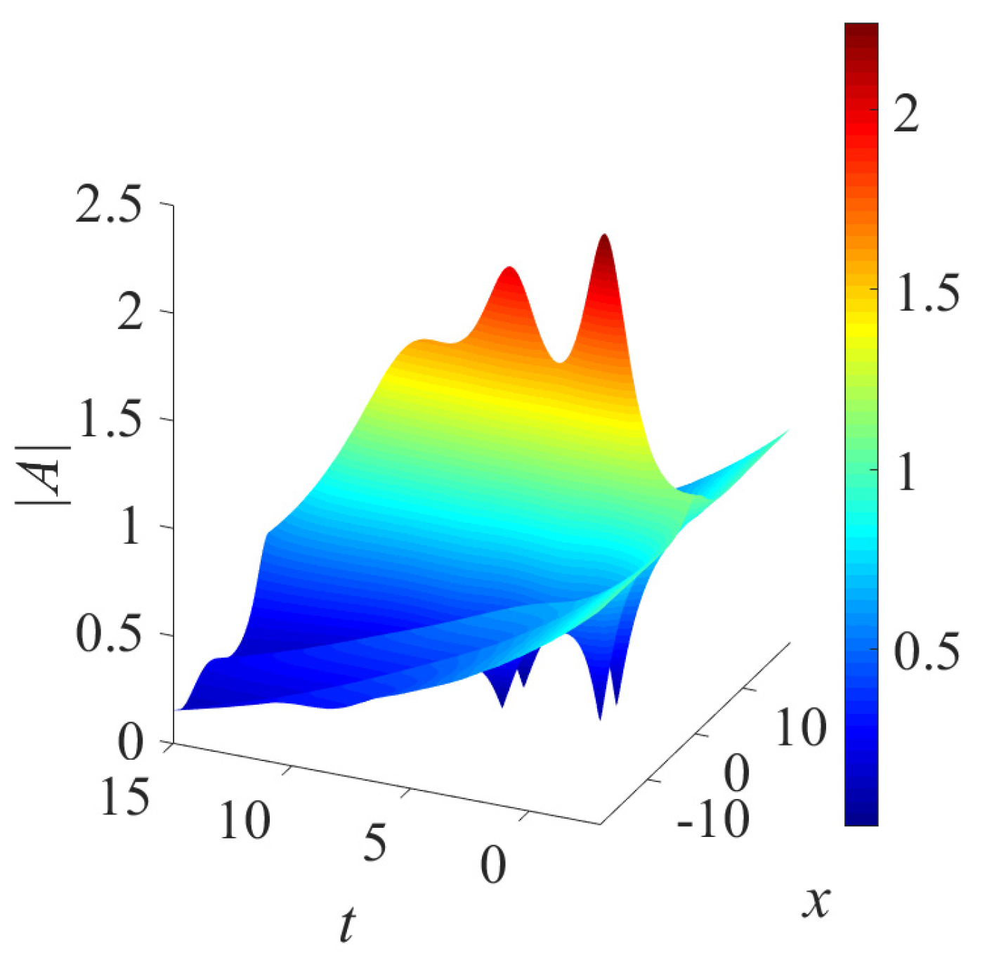
We shall first consider the simplest case where the medium possesses only a linear background loss or gain β, i.e., the variable linear gain and cubic gain functions vanish. When Equation (1) experiences a small loss (β < 0) globally, a rogue wave can still exist, but the maximum is reached at a later time as compared to the evolution governed by the NLSE (Equation (3)). The maximum attained by the rogue wave is also lowered, e.g., 1.7 for special choice of parameters as compared to 3.0 of the Peregrine breather of the NLSE [2,3] (Figure 1a). Conversely, a small gain (β > 0) will trigger a pulsating mode with growing peaks. As compared to the Peregrine breather, the wave reaches the peak amplitude before t = 0 and attains an amplitude greater than 4.1 (Figure 1b). Due to the presence of the gain, the spatially localized pulse does not decay back to the constant background plane wave, but instead evolves into multiple peaks with increasing amplitude.
2.3. Cubic Background Gain
Next, we consider the combined effect of cubic background gain and linear background loss (β < 0), or analytically, α(x, t) = α0 and γ ≡ 0. When the cubic gain is small, a rogue wave can still be observed and attains a maximum greater than that of the case with linear loss only (Figure 2a). However, for larger cubic gain α0, the growing peaks will eventually cause the solution to break down. This highlights the difference between linear and cubic amplification rates.
For specific values of amplitude, plane wave solutions exist but are unstable under the presence of dissipation. Mathematically,
is a stationary plane wave in the focusing regime. From linear stability analysis, it can be shown that the plane wave is modulationally unstable (Figure 2b). Recently, the role of baseband modulation instability in the generation of rogue waves was established for several integrable systems [35,36,37]. In other words, rogue waves can be triggered from a plane wave by a long wave disturbance [36,37]. Starting from the following initial condition, (Acw is the background continuous wave)
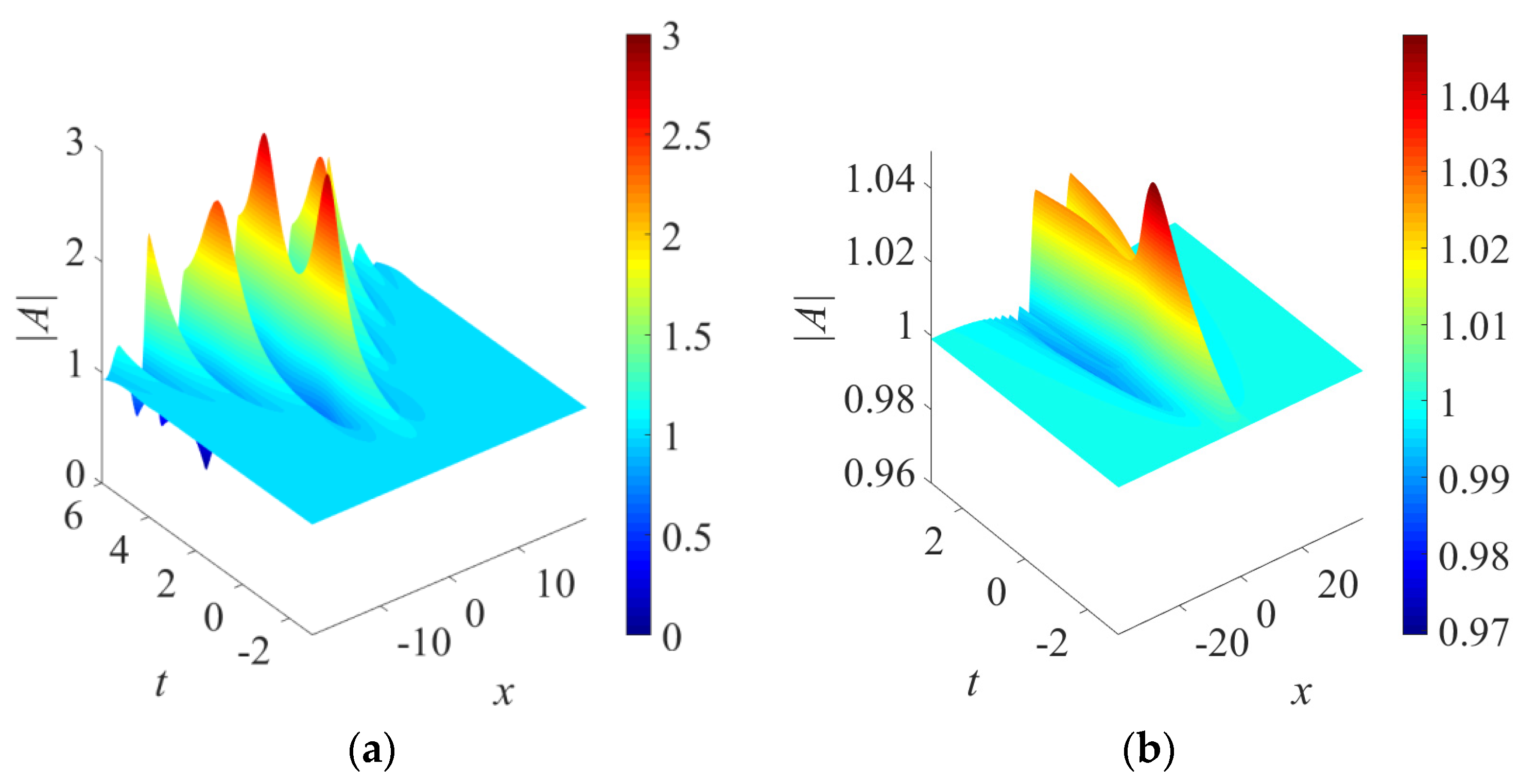
localized modes can be observed (Figure 2c). With a larger baseband increment (Figure 2b), rogue wave modes can be generated in a shorter time period (Figure 2d) [36]. Some structures with waveforms similar to a second order rogue wave can be observed at approximately t = 6.6.
3. Gain Localized in Space
The effect of a Gaussian gain localized in space is considered next. We utilize the terms ‘linear/cubic gain’ which more precisely would mean respectively, according to Equation (1), as ‘gain from external input proportional to the first/cubic power of the amplitude (A) but modulated in space (x) and time (t) by the function γ(x, t)/α(x, t)’.
3.1. Linear Gain
Consider a linear gain function localized in space but independent of time as described by a Gaussian function in x, i.e.,
where ε represents the ‘width’ of the Gaussian function and the parameter γ1 measures the maximum for a fixed ε. This gain will not lead to indefinite growth as it is balanced by the background loss β < 0.
This localized gain can compensate for the loss in the bulk of the medium and shorten the delay in reaching the maximum due to the background dissipation. For the numerical example as shown in Figure 3, this maximum is attained at t ≈ 0.4 (Figure 3a), which is sooner than the time necessary (at t ≈ 0.8 in Figure 1a) for the case without the Gaussian gain. Obviously, a greater maximum can be attained as compared to the case with background loss only (Figure 1a). With a fixed total gain but a greater maximum net gain, i.e., an amplification function corresponding to a smaller ε, the peak of the rogue wave increases.
Emergence of a Pinned Mode
However, when the gain is large enough, a pinned mode localized in space with a stationary waveform will become the dominant feature (Figure 3c). There are two possible scenarios for the generation of a pinned mode, namely, a sufficiently large total gain γ1 or a sufficiently small ε. For a fixed γ1, a smaller ε gives a sharper peak with greater maximum gain in Equation (4). When the maximum gain is large enough, the rogue wave absorbs the energy and grows into a pinned mode (Figure 3c). From our numerical results, the pinned mode tends to be a very narrow pulse. Resolution may be an issue and adaptive grids should perhaps be employed in future studies.
3.2. Cubic Gain
Similarly, consider a cubic gain function localized in space as given by,
where the gain is in competition with the background loss β < 0. For a sufficiently large cubic gain, the rogue wave will not subside. Instead, a finite number of peaks with decaying maximum displacements follow the major peak (Figure 4). When the gain is further increased, more peaks are generated and the maximum amplitude increases. Eventually, the cubic gain will cause the wave amplitude to attain indefinitely large amplitude, provided that α1 is sufficiently large. This blow up occurs at a relatively small gain parameter α1 which is reasonable as the growth rate is cubic.
4. Gain Localized in Both Space and Time
Finally, the effect of a gain localized in both space and time is considered. Instead of using a two-dimensional Gaussian gain, we consider a ‘rogue gain’. The amplification rate is localized in both the temporal and spatial domains, which is similar in nature to the rogue wave itself. More precisely, we consider
which is the amplitude of a Peregrine breather as given in Equation (2), with the coefficient of cubic nonlinearity replaced by σ0 and the background amplitude ρ is normalized to unity.
4.1. Linear Gain
Consider the following linear gain function
where γ2 is a scaling constant. The net background gain as u0 decays to unity is given by γ2 + β and the maximum gain 3γ2 + β is attained at the origin. The value of the parameter σ0 determines the rate of change in the gain function only. For a smaller σ0, the gain function increases to the maximum value more rapidly.
Recovery of a Rogue Wave from a Pinned Mode
Remarkably, by restricting the net linear gain to a short period of time only, the rogue wave can be recovered from the otherwise pinned mode discussed in the previous section. The idea is illustrated here with the numerical example discussed in Figure 3c,d. By choosing a net gain profile (Figure 5b) with the same maximum gain and background loss as that of Figure 3d, the pinned mode formed by the spatially localized gain of Figure 3c is destroyed. A rogue wave can thus be recovered by a ‘rogue’ gain function (Figure 5a).
Formation of Breather from Localized Gain with Negligible Background Loss
In the special case where the net gain exists only in a spatially localized region (Figure 5d), the rogue wave evolves into a Kuznetsov-Ma soliton pulsating in the time domain (Figure 5c). In other words, when the background loss goes to zero asymptotically (γ2 = −β), the localized gain near the origin will trigger the rogue wave to evolve into a breather propagating in the temporal domain instead of decaying back to the background. A pulsating mode with growing peaks can also be observed in a system with constant background gain as discussed in Section 2. The result here shows that a gain function restricted to a finite region can have a similar effect but the growth in amplitude ceases once the gain vanishes.
Suppression of a Rogue Wave
As discussed in Section 2, a background loss can lower the amplitude of the rogue wave and delay its formation. If the dissipative effect is further enhanced through a ‘rogue loss’ in the region where the Peregrine breather should form, the formation of rogue wave is suppressed (Figure 6a,b). We should emphasize that the effect of the background loss is essential. Consider an alternative system, where the dissipation exists only in the localized region, i.e., γ2 is taken as negative and the background loss is balanced by β > 0 (Figure 6d). Although there is a localized loss, the rogue wave can still survive. As compared to the case with constant background loss (Section 2), the peak of the rogue wave still maintains a relatively high value. This highlights the importance of a constant background loss in the suppression of a rogue wave. Furthermore, the two minima in Equation (6) form two extrema in localized gain due to the negative sign of γ2. As a result, two peaks are generated and follow the rogue wave to form a triangular train of rogue waves (Figure 6c).
Excitation from Continuous Waves
Alternatively, we test the impact of a ‘rogue gain’ on the dynamical properties of continuous waves. A continuous wave of NLSE is first taken as the initial condition in the computations [37]. In the focusing regime (σ > 0), where the Peregrine breather exists in the context of NLSE, a triangular train of peaks with waveform similar to rogue waves is generated (Figure 7a). However, in the defocusing regime of NLSE (σ < 0), where the Peregrine breather normally is not permitted, similar pulses cannot be generated. The ‘rogue gain’ gives rise to a small amplitude peak which does not decay back to the background immediately (Figure 7b). Instead, the peak splits into two soliton-like beams. Similar entities are observed in systems with nonlinearity and dispersion management [38].
4.2. Cubic Gain
Similarly, consider a ‘rogue-like’ cubic gain function given by
where α2 is a scaling constant. The effect of the cubic gain is much stronger than that of the linear gain. As a result, many features discussed for the case of linear gain do not hold for the current setting with cubic gain. For instance, the wave amplitude still blows up, even when the gain is restricted to the ‘rogue’ region only. This is in great contrast to the linear gain case when the rogue wave can be recovered from a pinned mode under a rogue gain. Secondly, trains of rogue waves cannot be generated from continuous waves of the NLSE. The perturbed continuous waves do grow indefinitely (‘blow up’), through a rapid increase of intensity.
5. Conclusions
The generation and dynamics of rogue waves in a dissipative medium governed by a complex Ginzburg-Landau equation have been investigated. Localized modes in systems with dissipation or gain have been pursued actively over the years. Dissipative defect modes can be found in optical lattices imprinted in focusing or defocusing cubic nonlinear media [39]. Solitons can also be amplified in the presence of external energy input, e.g., an appropriate gain given to a spatial soliton in a quadratic nonlinear medium may lead to redistribution of energy among various modes [40]. From a general perspective in the studies of solitons, insight and understanding in the generation and stability of solitons have been achieved through these nonlinear Schrödinger and complex Ginzburg-Landau equations [29].
A computational approach was adopted here to study the robustness of the Peregrine breather in a dissipative system. Several forms of the gain function were considered, namely, a constant background gain, a Gaussian gain localized in space, and a ‘rogue gain’ localized in both space and time. Moreover, both linear and cubic gain functions were studied. In most cases, the gain was balanced by a background loss. Although ingenious transformations can provide analytical models of rogue waves, one drawback in performing such transformations is that these variable coefficients may have to fulfill certain conditions [30,31,32,33,34]. As a result, the exact form of the gain cannot be arbitrary. The merit of a numerical approach is that there is no such restriction on the form of external energy input. The computational studies should enable us to obtain further insight into the problem.
For the simplest case where the linear gain or loss is constant throughout the domain, the gain (loss) increases (decreases) the maximum amplitude attained by the rogue wave and shortens (lengthens) the time necessary to reach the maximum. Moreover, a constant background gain will feed energy into other disturbances associated with the rogue wave, leading to multiple peaks with increasing amplitude subsequent to the occurrence of the rogue wave.
Secondly, a Gaussian gain localized in space with a constant background loss was considered. Rogue waves gain energy and grow into a pinned mode provided that the maximum linear gain is sufficiently large. However, the rogue wave can be recovered by restricting the localized gain to a finite time interval which we termed a ‘rogue gain’. Furthermore, in the focusing regime, such ‘rogue gain’ can generate trains of ‘rogue-wave-like’ entities from a continuous wave initial condition.
On the other hand, the formation of rogue wave is suppressed if the dissipation is sufficiently strong in the localized region. Both the background and local dissipative effects are essential to destroy the rogue wave. The mere existence of loss in the localized region, where the rogue wave evolves, may not be sufficient to annihilate it and thus the dynamics is indeed intriguing.
Both linear and cubic gains were investigated. Analytically, it is then obvious that the latter will overwhelm the former if the amplitude is large enough. When the cubic gain is sufficiently strong, the rogue wave will grow indefinitely and will cause the governing equation and the solution to break down. For scenarios with linear growth only, several peaks with increasing maximum can be formed but the amplitude remains finite.
In the present work, the cubic nonlinearity was taken as a positive constant but further exotic combinations of dispersion, nonlinearity, gain, and loss functions will constitute challenging issues for researchers. The role of dispersion management in the dynamics of rogue wave in a dissipative medium remains to be investigated [38]. Secondly, coupled systems where the gain and loss are balanced between the cores can be considered in the future [41]. Furthermore, the sandwich effect of a linear and quintic gain (or loss) on the cubic gain can be studied too [41,42,43]. The effect of an oscillatory gain or loss can be investigated [43,44]. Finally, the effect of an asymmetric gain or two hot spots can be pursued [22]. Computational studies of rogue waves have been actively pursued both from theoretical perspectives and in application settings [45,46]. Although we focus on computational studies on robustness here, other approximation techniques like adiabatic approximation might also be valuable [47,48,49,50,51]. A simplified version for the case of weak energy input and comparisons with numerical simulations are discussed in Appendix A. Further efforts on studies of rogue wave systems with gain/loss will definitely be fruitful in the future.
Author Contributions
Conceptualization, K.W.C.; Methodology, H.N.C. and K.W.C.; Software, H.N.C.; Formal Analysis, H.N.C. and K.W.C.; Writing-Review & Editing, H.N.C. and K.W.C.
Funding
Partial financial support has been provided by the Research Grants Council contract HKU17200815 and HKU17200718.
Conflicts of Interest
The authors declare no conflict of interest.
Appendix A
The adiabatic approximation is a commonly used scheme in estimating properties of wave dynamics or propagation through slowly varying media. While an elaborate analysis might be involved, the case of weak gain or loss can be illustrated through a combination of theoretical and numerical approaches here. For this purpose we consider
where μ << 1 will denote a weak gain/loss depending on the sign of β0. We assume that the wave dynamics will then be governed by a conventional rogue wave, uPB given by the Peregrine breather (Equation (2)) multiplied by a slowly varying envelope of the form exp(μz0t) for a complex z0, i.e.,
A = exp(μz0t) uPB.
Substituting this into the governing equation and retaining terms of order μ only, we get
Re(z0) = β0.
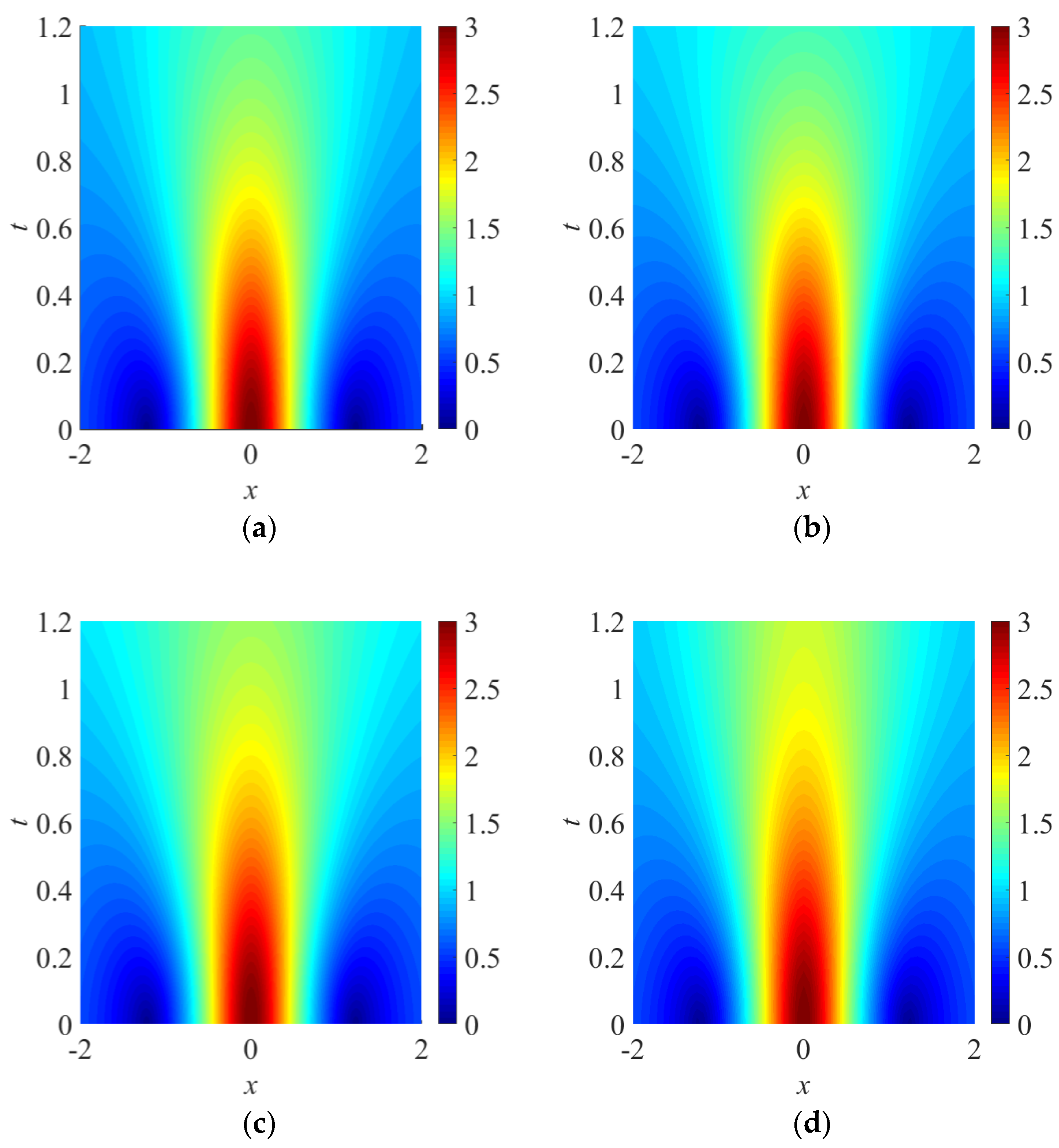
Numerical simulations with the actual governing equations as in the main text and direct evaluation using the adiabatic approximation Equation (A2) will now be compared (Figure A1). The absolute percentage errors at certain time instances are shown in Table A1. The results are in good agreement and the errors match the order of perturbation.
Figure A1.
Comparisons between the adiabatic approximation of the amplitude and results from a direct numerical simulation: Energy loss with β0 = −1 and μ = 0.05, (a) the adiabatic approximation given by Equation (A2) and (b) direct numerical simulation; Energy gain with β0 = 1 and μ = 0.05, (c) the adiabatic approximation and (d) direct numerical simulation; The maximum amplitudes obtained from the adiabatic approximations and direct simulations are in good agreement.

Table A1.
The amplitude of the wave packet at x = 0, |A(0,t)|: Comparisons between the approaches of adiabatic approximations and direct numerical simulations.
Table A1.
The amplitude of the wave packet at x = 0, |A(0,t)|: Comparisons between the approaches of adiabatic approximations and direct numerical simulations.
| β0 | t | Adiabatic Approximation of |A(0,t)| by Equation (A2) | Numerical Approximation of |A(0,t)| by Simulation | Absolute Percentage Error | |
|---|---|---|---|---|---|
| 0.05 | −1 | 0.5 | 2.18 | 2.15 | 1.4% |
| 0.05 | −1 | 1 | 1.53 | 1.47 | 4.08% |
| 0.05 | 1 | 0.5 | 2.29 | 2.33 | 1.72% |
| 0.05 | 1 | 1 | 1.7 | 1.79 | 5.03% |
References
- Aranson, I.S.; Kramer, L. The world of the complex Ginzburg-Landau equation. Rev. Mod. Phys. 2002, 74, 99–143. [Google Scholar] [CrossRef] [Green Version]
- Dysthe, K.; Krogstad, H.E.; Müller, P. Oceanic rogue waves. Annu. Rev. Fluid Mech. 2008, 40, 287–310. [Google Scholar] [CrossRef]
- Onorato, M.; Residori, S.; Bortolozzo, U.; Montina, A.; Arecchi, F.T. Rogue waves and their generating mechanisms in different physical contexts. Phys. Rep. 2013, 528, 47–89. [Google Scholar] [CrossRef]
- Dudley, J.M.; Dias, F.; Erkintalo, M.; Genty, G. Instabilities, breathers and rogue waves in optics. Nat. Photonics 2014, 220, 755–764. [Google Scholar] [CrossRef]
- Akhmediev, N.; Kibler, B.; Baronio, F.; Belić, M.; Zhong, W.-P.; Zhang, Y.; Chang, W.; Soto-Crespo, J.M.; Vouzas, P.; Grelu, P.; et al. Roadmap on optical rogue waves and extreme events. J. Opt. 2016, 18, 063001. [Google Scholar] [CrossRef] [Green Version]
- Chen, S.; Baronio, F.; Soto-Crespo, J.M.; Grelu, P.; Mihalache, D. Versatile rogue waves in scalar, vector, and multidimensional nonlinear systems. J. Phys. A: Math. Theor. 2017, 50, 463001. [Google Scholar] [CrossRef] [Green Version]
- Zhong, W.P.; Belić, M.R.; Huang, T. Rogue wave solutions to the generalized nonlinear Schrödinger equation with variable coefficients. Phys. Rev. E 2013, 87, 065201. [Google Scholar] [CrossRef] [PubMed]
- Manikandan, K.; Muruganandam, P.; Senthilvelan, M.; Lakshmanan, M. Manipulating localized matter waves in multicomponent Bose-Einststen condensates. Phys. Rev. E 2016, 93, 032212. [Google Scholar] [CrossRef] [PubMed]
- Cheng, X.; Wang, J.; Li, J. Controllable rogue waves in coupled nonlinear Schrödinger equations with varying potentials and nonlinearities. Nonlinear Dyn. 2014, 77, 545–552. [Google Scholar] [CrossRef]
- Tlidi, M.; Panajotov, K. Two-dimensional dissipative rogue waves due to time-delayed feedback in cavity nonlinear optics. Chaos 2017, 27, 013119. [Google Scholar] [CrossRef] [PubMed] [Green Version]
- Tlidi, M.; Panajotov, K.; Ferré, M.; Clerc, M.G. Drifting cavity solitons and dissipative rogue waves induced by time-delayed feedback in Kerr optical frequency comb and in all fiber cavities. Chaos 2017, 27, 114312. [Google Scholar] [CrossRef] [PubMed]
- Panajotov, K.; Clerc, M.G.; Tlidi, M. Spatiotemporal chaos and two-dimensional dissipative rogue waves in Lugiato-Lefever model. Eur. Phys. J. D 2017, 71, 176. [Google Scholar] [CrossRef]
- Tlidi, M.; Gandica, Y.; Sonnino, G.; Averlant, E.; Panajotov, K. Self-replicating spots in the Brusselator model and extreme events in the one-dimensional case with delay. Entropy 2016, 18, 64. [Google Scholar] [CrossRef]
- Liu, M.; Luo, A.P.; Xu, W.C.; Luo, Z.C. Dissipative rogue waves induced by soliton explosions in an ultrafast fiber laser. Opt. Lett. 2016, 41, 3912–3915. [Google Scholar] [CrossRef] [PubMed]
- Liu, M.; Cai, Z.R.; Hu, S.; Luo, A.P.; Zhao, C.J.; Zhang, H.; Xu, W.C.; Luo, Z.C. Dissipative rogue waves induced by long-range chaotic multi-pulse interactions in a fiber laser with a topological insulator-deposited microfiber photonic device. Opt. Lett. 2015, 40, 4767–4770. [Google Scholar] [CrossRef] [PubMed]
- Peng, J.; Tarasov, N.; Sugavanam, S.; Churkin, D. Rogue waves generation via nonlinear soliton collision in multiple-soliton state of a mode-locked fiber laser. Opt. Expr. 2016, 24, 24256–24263. [Google Scholar] [CrossRef] [PubMed]
- Soto-Crespo, J.M.; Devine, N.; Akhmediev, N. Dissipative solitons with extreme spikes: Bifurcation diagrams in the anomalous dispersion. J. Opt. Soc. Am. B 2017, 34, 1542–1549. [Google Scholar] [CrossRef]
- Chang, W.; Soto-Crespo, J.M.; Vouzas, P.; Akhmediev, N. Spiny solitons and noise-like pulses. J. Opt. Soc. Am. B 2015, 32, 1377–1383. [Google Scholar] [CrossRef]
- Shemer, L.; Alperovich, L. Peregrine breather revisited. Phys. Fluids 2013, 25, 051701. [Google Scholar] [CrossRef] [Green Version]
- Hu, Z.; Tang, W.; Xue, H.X.; Zhang, X.Y. Numerical study of rogue waves as nonlinear Schrödinger breather solutions under finite water depth. Wave Motion 2015, 52, 81–90. [Google Scholar] [CrossRef]
- Lam, C.K.; Malomed, B.A.; Chow, K.W.; Wai, P.K.A. Spatial solitons supported by localized gain in nonlinear optical waveguides. Eur. Phys. J. Spec. Top. 2009, 173, 233–243. [Google Scholar] [CrossRef]
- Tsang, C.H.; Malomed, B.A.; Lam, C.K.; Chow, K.W. Solitons pinned to hot spots. Eur. Phys. J. D 2010, 59, 81–89. [Google Scholar] [CrossRef]
- Davey, A.; Stewartson, K. 3-Dimensional packets of surface-waves. Proc. R. Soc. 1974, 338, 101–110. [Google Scholar] [CrossRef]
- Ablowitz, M.J.; Segur, H. Evolution of packets of water waves. J. Fluid Mech. 1979, 92, 691–715. [Google Scholar] [CrossRef]
- Chabchoub, A.; Hoffmann, N.; Onorato, M.; Akhmediev, N. Super rogue waves: Observation of a higher-order breather in water waves. Phys. Rev. X 2012, 2, 011015. [Google Scholar] [CrossRef]
- Dong, G.; Liao, B.; Ma, Y.; Perlin, M. Experimental investigation of the Peregrine breather of gravity waves on finite water depth. Phys. Rev. Fluids 2018, 3, 064801. [Google Scholar] [CrossRef]
- Menyuk, C.R.; Schiek, R.; Torner, L. Solitary waves due to χ(2): χ(2) cascading. J. Opt. Soc. Am. B 1994, 11, 2434–2443. [Google Scholar] [CrossRef]
- Chowdhury, N.A.; Mannan, A.; Mamun, A.A. Rogue waves in space dusty plasma. Phys. Plasma 2017, 24, 113701. [Google Scholar] [CrossRef]
- Malomed, B.A.; Mihalache, D.; Wise, F.; Torner, L. Spatiotemporal optical solitons. J. Opt. B Quantum Semiclass. Opt. 2005, 7, R53–R72. [Google Scholar] [CrossRef]
- Serkin, V.N.; Hasegawa, A. Novel soliton solutions of the nonlinear Schrödinger equation model. Phys. Rev. Lett. 2000, 85, 4502–4505. [Google Scholar] [CrossRef] [PubMed]
- Wang, L.; Zhang, J.H.; Liu, C.; Li, M.; Qi, F.H. Breather transition dynamics, Peregrine combs and walls, and modulation instability in a variable-coefficient nonlinear Schrödinger equation with high-order effects. Phys. Rev. E 2016, 93, 062217. [Google Scholar] [CrossRef] [PubMed]
- Zhong, W.P.; Belić, M.; Malomed, B.A. Rogue waves in a two-component Manakov system with variable coefficients and an external potential. Phys. Rev. E 2015, 92, 053201. [Google Scholar] [CrossRef] [PubMed] [Green Version]
- Yang, Z.; Zhong, W.P.; Belić, M.; Zhang, Y. Controllable optical rogue waves via nonlinearity management. Opt. Express 2018, 26, 7587–7597. [Google Scholar] [CrossRef] [PubMed]
- Estelle Temgoua, D.D.; Tchoula Tchokonte, M.B.; Kofane, T.C. Combined effects of nonparaxiality, optical activity, and walk-off on rogue wave propagation in optical fibers filled with chiral materials. Phys. Rev. E 2018, 97, 042205. [Google Scholar] [CrossRef] [PubMed]
- Baronio, F.; Chen, S.; Grelu, P.; Wabnitz, S.; Conforti, M. Baseband modulation instability as the origin of rogue waves. Phys. Rev. A 2015, 91, 033804. [Google Scholar] [CrossRef]
- Chan, H.N.; Chow, K.W. Rogue waves for an alternative system of coupled Hirota equations: Structural robustness and modulation instabilities. Stud. Appl. Math. 2017, 139, 78–103. [Google Scholar] [CrossRef]
- Chan, H.N.; Chow, K.W. Rogue wave modes for the coupled nonlinear Schrödinger system with three components: A computational study. Appl. Sci. 2017, 7, 559. [Google Scholar] [CrossRef]
- Cuevas-Maraver, J.; Malomed, B.A.; Kevrekidis, P.G.; Frantzeskakis, D.J. Stabilization of the Peregrine soliton and Kuznetsov-Ma breathers by means of nonlinearity and dispersion management. Phys. Lett. A 2018, 382, 968–972. [Google Scholar] [CrossRef]
- Kartashov, Y.V.; Konotop, V.V.; Vysloukh, V.A.; Torner, L. Dissipative defect modes in periodic structures. Opt. Lett. 2010, 35, 1638–1640. [Google Scholar] [CrossRef] [PubMed]
- Torner, L. Amplification of quadratic solitons. Opt. Commun. 1998, 154, 59–64. [Google Scholar] [CrossRef]
- Malomed, B.A. Spatial solitons supported by localized gain. J. Opt. Soc. Am. B 2014, 31, 2460–2475. [Google Scholar] [CrossRef]
- Descalzi, O.; Cartes, C. Stochastic and higher-order effects on exploding pulses. Appl. Sci. 2017, 7, 887. [Google Scholar] [CrossRef]
- He, J.; Malomed, B.A.; Mihalache, D. Localized modes in dissipative lattice media: An overview. Philos. Trans. R. Soc. A 2014, 372, 20140017. [Google Scholar] [CrossRef] [PubMed]
- Kartashov, Y.V.; Torner, L. Rotation-managed dissipative solitons. Opt. Lett. 2013, 38, 2317–2320. [Google Scholar] [CrossRef] [PubMed] [Green Version]
- Fochesato, C.; Grilli, S.; Dias, F. Numerical modeling of extreme rogue waves generated by directional energy focusing. Wave Motion 2007, 44, 395–416. [Google Scholar] [CrossRef]
- Porubov, A.V.; Tsuji, H.; Lavrenov, I.V.; Oikawa, M. Formation of the rogue wave due to non-linear two-dimensional waves interaction. Wave Motion 2005, 42, 202–210. [Google Scholar] [CrossRef]
- Gerdjikov, V.S.; Todorov, M.D.; Kyuldjiev, A.V. Adiabatic interactions of Manakov solitons-Effects of cross-modulation. Wave Motion 2017, 71, 71–81. [Google Scholar] [CrossRef]
- Dang Koko, A.; Tabi, C.B.; Ekobena Fouda, H.P.; Mohamadou, A.; Kofané, T.C. Nonlinear charge transport in the helicoidal DNA molecule. Chaos 2012, 22, 043110. [Google Scholar] [CrossRef] [PubMed]
- Kivshar, Y.S.; Malomed, B.A. Dynamics of solitons in nearly integrable systems. Rev. Mod. Phys. 1989, 61, 763–915. [Google Scholar] [CrossRef]
- Böhm, M.; Mitschke, F. Solitons in lossy fibers. Phys. Rev. A 2007, 76, 063822. [Google Scholar] [CrossRef]
- Mitschke, F.; Mahnke, C.; Hause, A. Soliton content of fiber-optic light pulses. Appl. Sci. 2017, 7, 635. [Google Scholar] [CrossRef]
Figure 1.
Effect of linear background loss or gain (σ = 1, γ ≡ α ≡ 0): (a) β = −0.1; (b) β = 0.1.
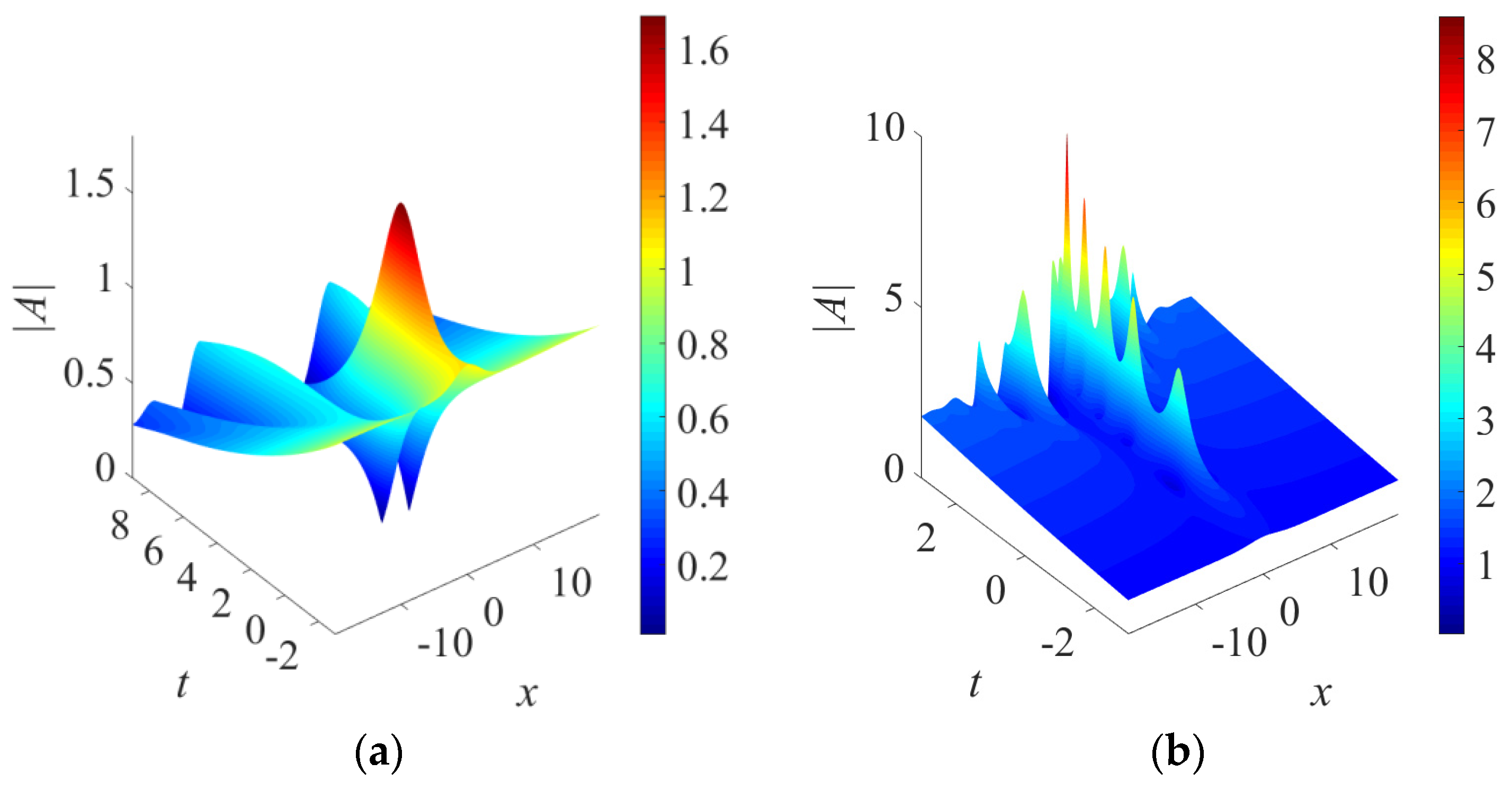
Figure 2.
(a) Effect of cubic background gain at σ = 1, β = −0.1, γ ≡ 0 and α0 = 0.01. (b) Modulation instability gain spectrum at σ = 1, β = −0.01, γ ≡ 0 and α0 = 0.01 (red dashed line); α0 = 0.002 (blue solid line). (c) Rogue wave generated from the plane wave by a baseband disturbance at σ = 1, β = −0.01, γ ≡ 0, α0 = 0.01, K = 0.1, b0 = 0.05. (d) For a system with a larger baseband increment, rogue-wave-like objects appear sooner. Parameters are the same as (c) except α0 = 0.002.
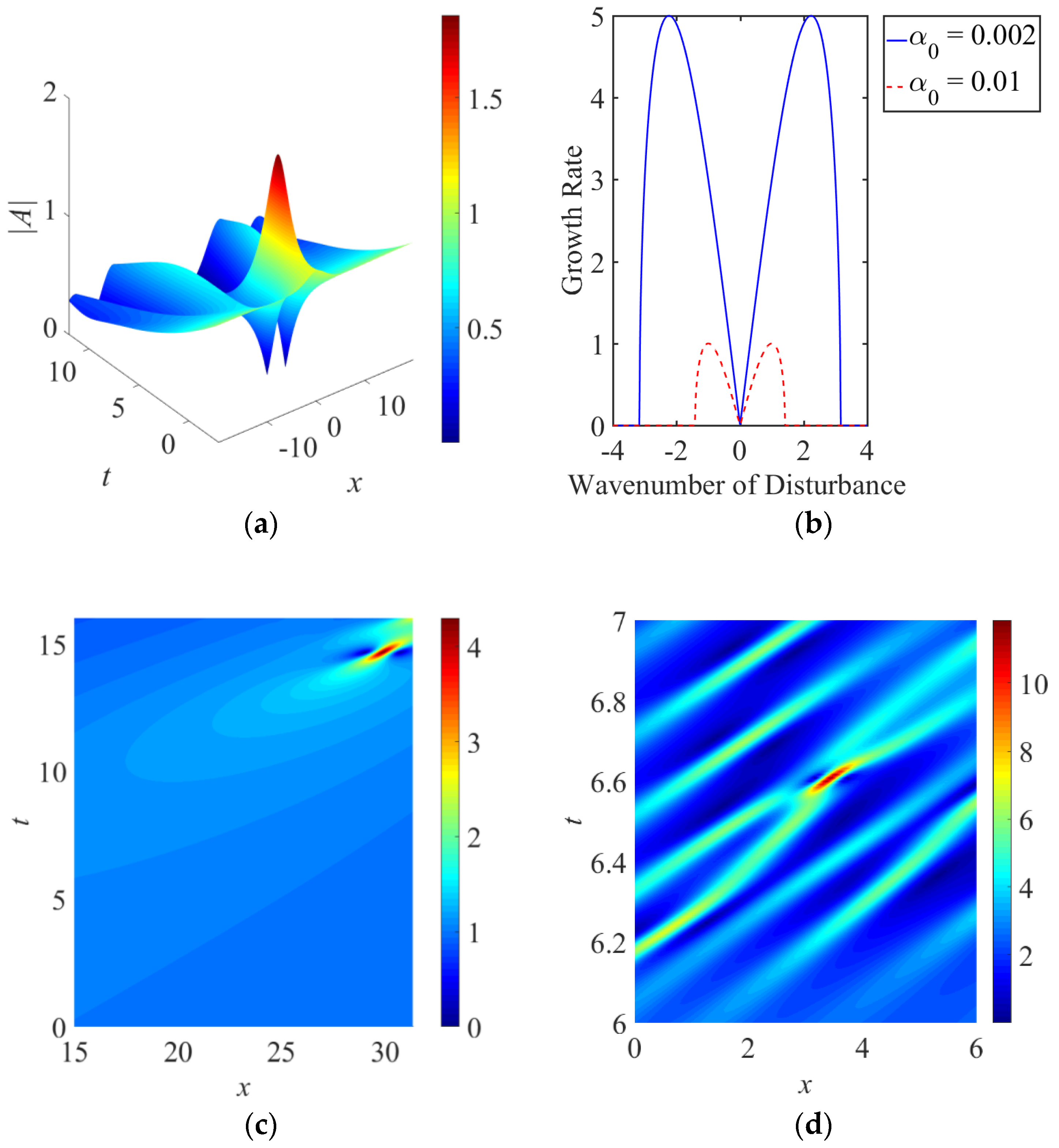
Figure 3.
Effect of linear gain localized in space (σ = 1, β = −0.1, ε = 0.1, α ≡ 0): (a) simulated result of a rogue wave and (b) the net gain at γ1 = 0.1; (c) simulated result of a pinned mode and (d) the net gain at γ1 = 0.2.
Figure 3.
Effect of linear gain localized in space (σ = 1, β = −0.1, ε = 0.1, α ≡ 0): (a) simulated result of a rogue wave and (b) the net gain at γ1 = 0.1; (c) simulated result of a pinned mode and (d) the net gain at γ1 = 0.2.
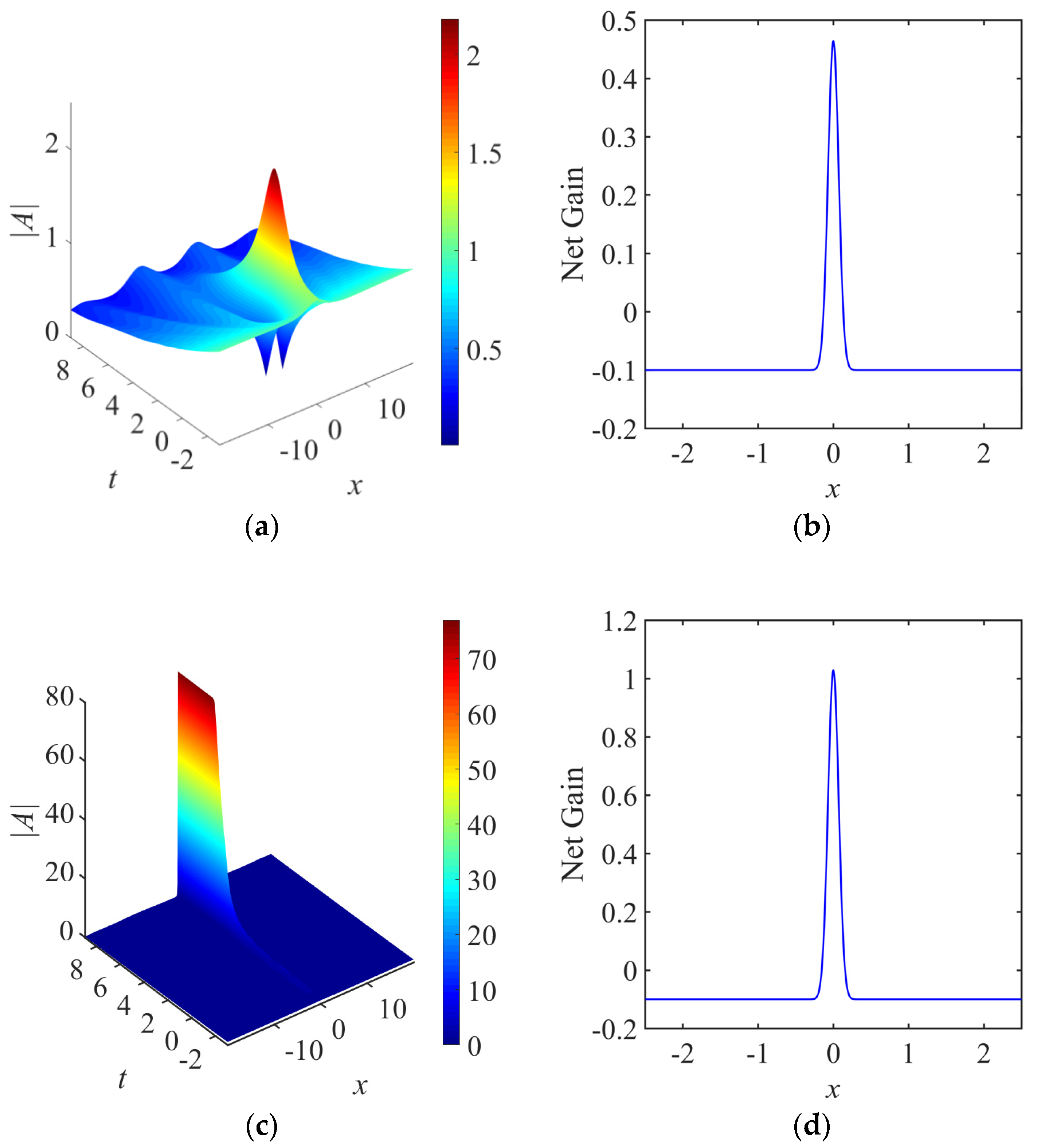
Figure 4.
Effect of cubic gain localized in space: simulated result of a rogue wave with multiple peaks at σ = 1, β = −0.1, γ ≡ 0, ε = 0.1 and α1 = 0.042.
Figure 4.
Effect of cubic gain localized in space: simulated result of a rogue wave with multiple peaks at σ = 1, β = −0.1, γ ≡ 0, ε = 0.1 and α1 = 0.042.

Figure 5.
Effect of linear gain localized in both space and time (σ = 1, α ≡ 0): (a) a recovered rogue wave at β = −0.6642, γ2 = 0.5642, σ0 = 20 and (b) the net gain at t = 0; (c) a Kuznetsov-Ma soliton at β = −0.1, γ2 = 0.1, σ0 = 1 and (d) the net gain.
Figure 5.
Effect of linear gain localized in both space and time (σ = 1, α ≡ 0): (a) a recovered rogue wave at β = −0.6642, γ2 = 0.5642, σ0 = 20 and (b) the net gain at t = 0; (c) a Kuznetsov-Ma soliton at β = −0.1, γ2 = 0.1, σ0 = 1 and (d) the net gain.
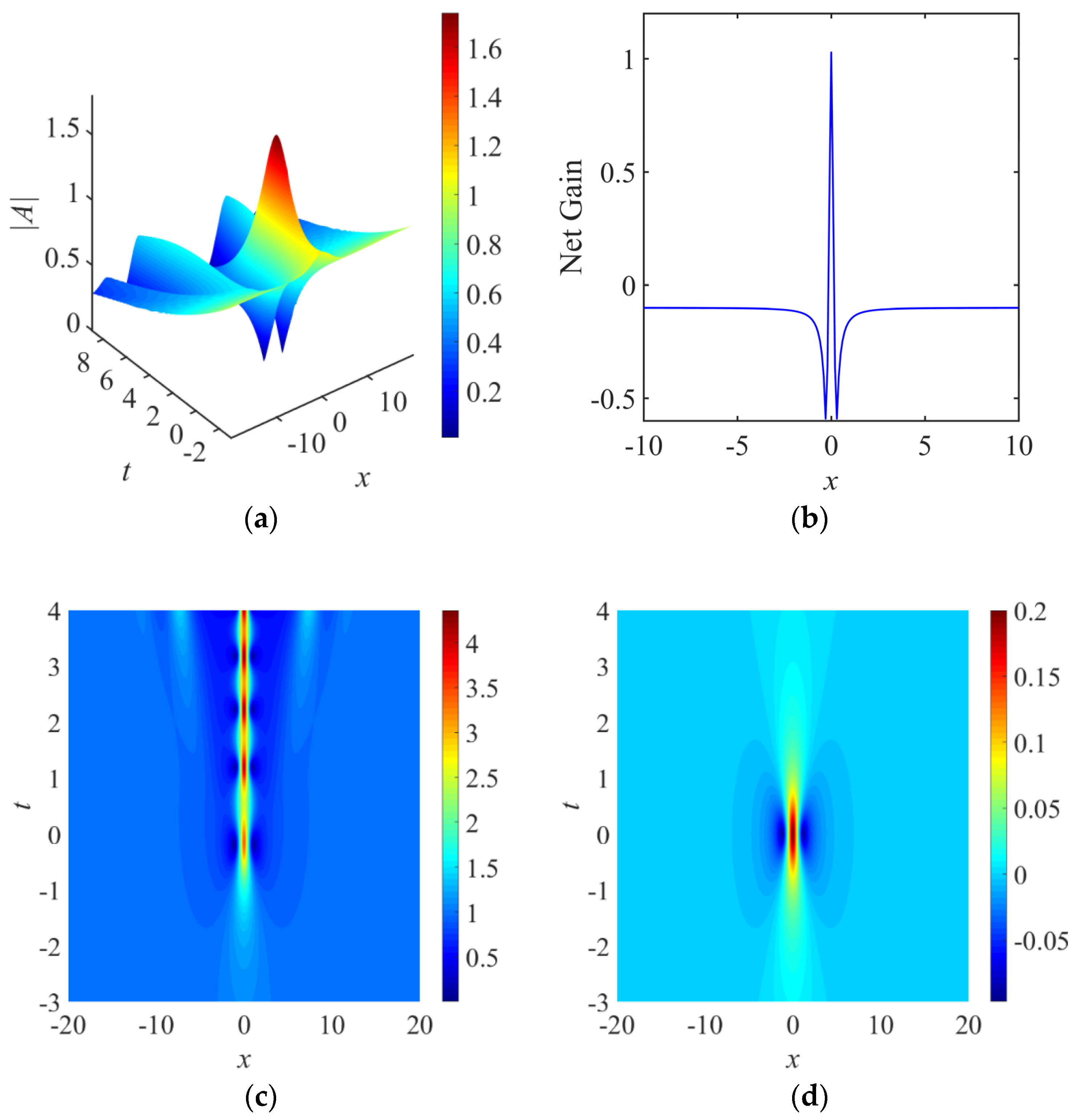
Figure 6.
Effect of linear gain localized in both space and time (σ = 1, α ≡ 0): (a) the formation of rogue wave is suppressed at β = 0, γ2 = −0.15, σ0 = 1 and (b) the net gain at t = 0; (c) a triangular train of rogue waves at β = 0.1, γ2 = −0.1, σ0 = 1 and (d) the net gain at t = 0.
Figure 6.
Effect of linear gain localized in both space and time (σ = 1, α ≡ 0): (a) the formation of rogue wave is suppressed at β = 0, γ2 = −0.15, σ0 = 1 and (b) the net gain at t = 0; (c) a triangular train of rogue waves at β = 0.1, γ2 = −0.1, σ0 = 1 and (d) the net gain at t = 0.
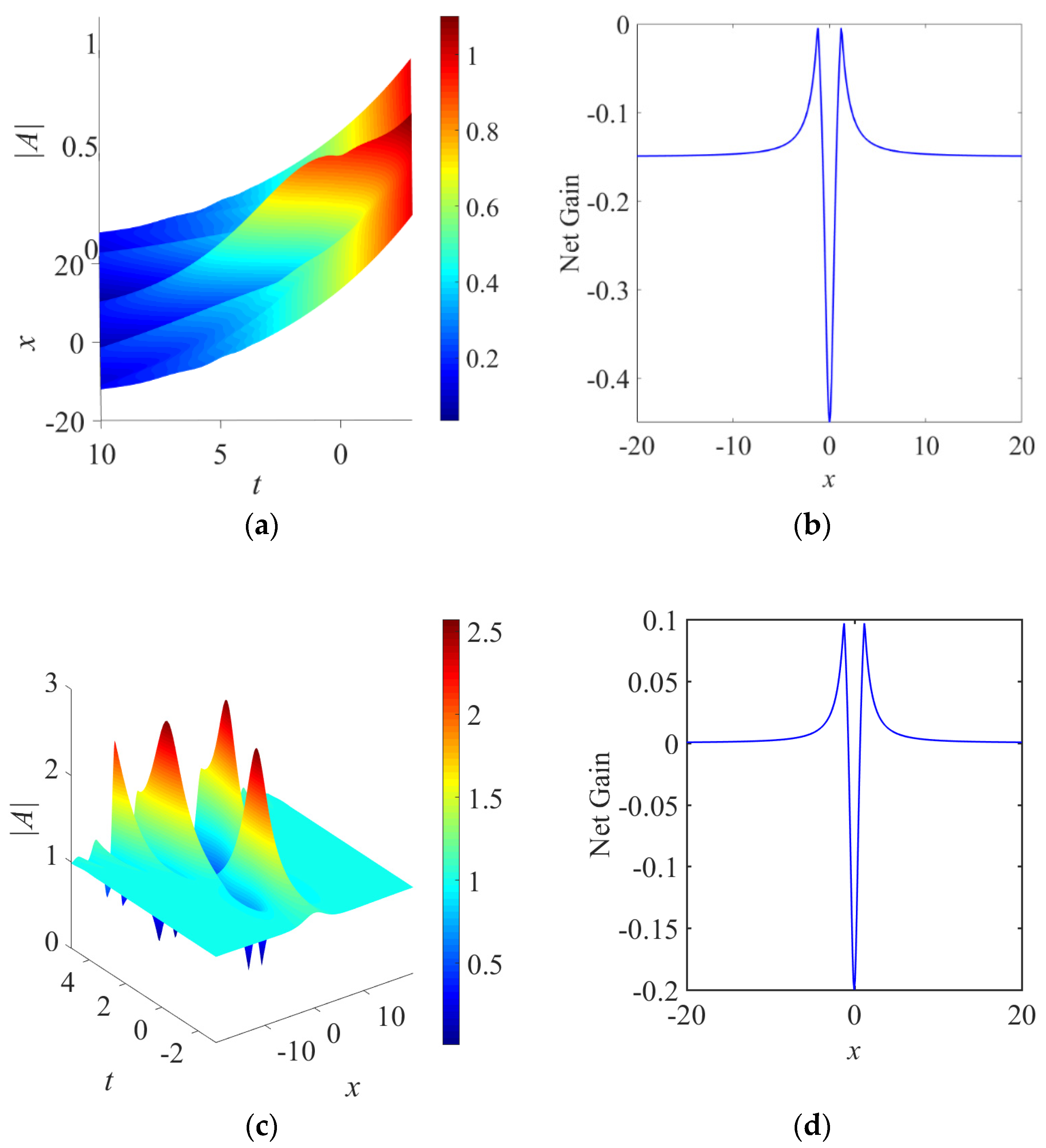
Figure 7.
Effect of linear gain localized in both space and time: (a) generation of rogue waves from continuous wave of the NLSE in the focusing regime σ = 1; (b) small amplitude peak generated in the defocusing regime σ = −1. (β = −0.1, σ0 = 1, γ2 = 0.1 and α ≡ 0 in both cases).
Figure 7.
Effect of linear gain localized in both space and time: (a) generation of rogue waves from continuous wave of the NLSE in the focusing regime σ = 1; (b) small amplitude peak generated in the defocusing regime σ = −1. (β = −0.1, σ0 = 1, γ2 = 0.1 and α ≡ 0 in both cases).

© 2018 by the authors. Licensee MDPI, Basel, Switzerland. This article is an open access article distributed under the terms and conditions of the Creative Commons Attribution (CC BY) license (http://creativecommons.org/licenses/by/4.0/).
Share and Cite
MDPI and ACS Style
Chan, H.N.; Chow, K.W. Numerical Investigation of the Dynamics of ‘Hot Spots’ as Models of Dissipative Rogue Waves. Appl. Sci. 2018, 8, 1223. https://doi.org/10.3390/app8081223
AMA Style
Chan HN, Chow KW. Numerical Investigation of the Dynamics of ‘Hot Spots’ as Models of Dissipative Rogue Waves. Applied Sciences. 2018; 8(8):1223. https://doi.org/10.3390/app8081223
Chicago/Turabian StyleChan, Hiu Ning, and Kwok Wing Chow. 2018. "Numerical Investigation of the Dynamics of ‘Hot Spots’ as Models of Dissipative Rogue Waves" Applied Sciences 8, no. 8: 1223. https://doi.org/10.3390/app8081223
Note that from the first issue of 2016, this journal uses article numbers instead of page numbers. See further details here.