Challenges and Limitations in the Identification of Acoustic Emission Signature of Damage Mechanisms in Composites Materials


Laboratory MATEIS, University of Lyon, INSA-Lyon, 69621 Villeurbanne, France
*
Author to whom correspondence should be addressed.
Appl. Sci. 2018, 8(8), 1267; https://doi.org/10.3390/app8081267
Submission received: 13 July 2018
/
Revised: 25 July 2018
/
Accepted: 27 July 2018
/
Published: 31 July 2018
(This article belongs to the Special Issue Damage Inspection of Composite Structures)
Abstract
:Acoustic emission is a part of structural health monitoring (SHM) and prognostic health management (PHM). This approach is mainly based on the activity rate and acoustic emission (AE) features, which are sensitive to the severity of the damage mechanism. A major issue in the use of AE technique is to associate each AE signal with a specific damage mechanism. This approach often uses classification algorithms to gather signals into classes as a function of parameters values measured on the signals. Each class is then linked to a specific damage mechanism. Nevertheless, each recorded signal depends on the source mechanism features but the stress waves resulting from the microstructural changes depend on the propagation and acquisition (attenuation, damping, surface interactions, sensor characteristics and coupling). There is no universal classification between several damage mechanisms. The aim of this study is the assessment of the influence of the type of sensors and of the propagation distance on the waveforms parameters and on signals clustering.
1. Introduction
Acoustic Emission (AE) is the transient elastic sound waves when a material undergoes stress. It is used as a Non-Destructive Testing technique to monitor damage in composites materials and structures [1,2,3,4]. Usually, piezoelectric sensors applied directly on the samples surface capture these elastic waves. The analysis of the collected data can be used to discriminate the sources of damage (matrix cracks, fibre breaks, fibre/matrix decohesion, delamination) and to determine the kinetics of the various degradation mechanisms during the lifetime. Indeed, the shape and the characteristics of the AE signals are directly dependent on the local damage mechanisms such as delamination, matrix cracking, fibre matrix debonding, fibre break and fibre pull-out. Therefore, it is realistic to consider that this signal contains some features representative of the source in such a manner that direct correlation exists between the damage mechanisms and the AE parameters. In this type of studies, a main assumption is done: signals are affected by propagation but they remain images of sources. Therefore, acoustic emission events can be classified using multivariable statistical analysis techniques and then attributed to a damage mechanism in the material [5,6,7,8,9,10,11,12]. The main assumption is: the acoustic signatures are unchanged during propagation and damage evolution. AE signals that have similar characteristics are grouped using a clustering method, based on similarity measures, in order to reveal the natural structure of data. This procedure is based on the representation of AE signals by relevant descriptors. The descriptors selection is an important step [13,14,15]. For the unsupervised pattern recognition, the descriptors should be relevant and limited in number. The possibility to identify AE signatures of damage mechanisms is an established field [5,6,7,8,9,10,11,12]. In most studies, the attribution of each class to a specific damage mechanism is based mainly on empirical approach and the validation of this labelling remains difficult and is still a challenge. In most works, the assignment of a signal to a damage mechanism is very difficult, if not impossible, to validate without any modelling [16,17,18,19]. Sause [16] models AE sources in a specimen for different damage mechanisms, as well as the signal propagation and the different elements of the acquisition chain by a finite element method. For each cluster and for each mechanism, he compares the experimental values of the signal descriptors with the theoretical values generated by the damage mechanism, which is affiliated to it. It can thus judge the relevance of its labelling.
Moreover, several authors use acoustic emission in the aim of prognostics, in order to make remaining useful lifetime previsions [8,20,21,22,23,24,25,26]. An estimate of the composite materials remaining lifetime can be considered based on a real-time tracking of the damage recorded by EA. In the context of the failure of the prediction of composite, Arumugan [23] predicted residual tensile strength of impacted carbon/epoxy laminates using an artificial neural network with AE data collected up to 50% of failure loads. The chosen descriptors are the cumulative counts and the amplitude. Several authors [24] used AE peak amplitude and energy parameter into neural network for predicting the tensile strength of carbon epoxy composites. For the specific study of CMCs (ceramic matrix composites) in fatigue, Momon et al. [25] introduced an indicator, denoted RAE, the coefficient of emission, which is shown to go through a minimum value of around 50–60% of the total test duration. Therefore, beyond 50% of the total test duration, a power law can model the criticality in order to evaluate time to failure. Study of the damage indices based on acoustic energy or parameters enlightens the damage evolution, enabling predictions of the remaining life [8,25,26].
In these studies, the wave from the source is altered during propagation and this aspect is very rarely taken into account. Indeed, the signal is modified during propagation (mode conversion, reflections, dispersion) and then by the acquisition system [27,28,29,30,31,32,33,34,35,36]. Aggelis et al. [30,31] show that the separation distance between the sensors is of paramount importance and it should be taken into account when crack mode estimation is attempted by experimental data. Hamstad et al. [32] carried out impact tests on 260 mm outer diameter pressure vessels made of a fibreglass/epoxy matrix composite. Their study focused on the effect of source/sensor distance. They are able to show that the characteristic parameters of waveforms such as amplitude, rise time, as well as the spectral content of the signals for identical sources are largely influenced by the sensor source distance. For small distances (less than 60 mm), the physical significance of an acoustic event can be evaluated only by taking into account the propagation. Thus, the same author [33] showed that the representations obtained by the continuous wavelet transform vary according to the type of AE source and the propagation distance between these sources and the sensors in aluminium plates. The analysed parameters are highly dependent on the material properties, the structure geometries, the sensor and the detection and analysis system. In addition, the state of damage of the material can affect AE signals [34,35]. All these evolutions make the interpretation of the signals very difficult. The specific values of the AE parameters are very sensitive to the experimental set up and conditions like geometries. Comparisons should be careful and only for exactly the same experimental conditions. In this context, the acoustic signature of a damage mechanism is not generalizable. The geometry of the sample is also an important parameter. Consequently, identification of the source and comparison with results from other tests performed under different conditions are difficult.
The influence of the mentioned experimental conditions should be investigated and taken into account to increase reliability. The objective of the paper is twofold (1) use artificial sources with acousto-ultrasonic (AU) technique to generate AE sources with specific characteristics in order to analyse the sensor response and (2) study the influence of the sensor, propagation and damage on AE features and clustering results.
Therefore, the first part of this paper is devoted to the study of the response of the sensor for artificial sources generated using an ultrasonic card. The AU technique consists in the excitation of the sample by a particular wave packet emitted from a sensor and the signal is recorded using an AE system. Artificial sources with different characteristics are created in undamaged state and during a mechanical test. Maillet et al. [37] develop a testing protocol that combines acousto-ultrasonic and acoustic emission monitoring, thus providing both global and local definite information on damage modes of SiCf/SiC minicomposites. Wave velocity measurements using acousto-ultrasonic allowed accurate location of AE sources by taking into account the damage dependence of wave velocity. In this study, the evolution of the waveforms as a function of the input characteristics and damage are investigated in order to guide pattern recognition techniques or the lifetime prediction based on the recorded energy.
The second part is dedicated to the influence of the type of sensor and the source-sensor distance in order to highlight the limitations of the identification of the acoustic emission signature of several damage mechanisms. The present study uses various sensors to investigate the effect of the sensor and the propagation distance. Four sensors monitor the same tensile test on several kinds of composite in order to point out the influence of the sensor and its position. AE signals received at the same position by two kinds of sensors are treated separately to examine the effect of the sensor on the AE features and on the results of classification. AE signals received at increasing distances (with and without waveguide) by the same type of sensors are analysed independently to examine the effects of travelling distance on the classification results. This study investigates from an experimental point of view the influence of sensor, propagation and damage on the AE features. In this paper, we are going to focus mainly on the evolution of amplitude, energy and frequency.
2. Materials and Experimental Procedure
2.1. Material and Mechanical Tests
Tensile tests are conducted at room temperature on several kinds of fibre composites, ceramic matrix composites (CMC) and organic matrix composites (OMC). All strain data are measured by clip on extensometer.
Tests are conducted on CMC, a multi-layered [Si-B-C] matrix reinforced with Hi-Nicalon fibres and a carbon interphase layer (SAFRAN CERAMICS Bordeaux, France). The composite contains a volumic fraction of fibres equal to 35%. In this study, all the specimens have a dog-bone shape with a thickness of 3.5 mm (200 mm × 24 mm) and a gauge section of 60 mm × 16 mm. On CMC composite, tensile tests are conducted at room temperature and static fatigue tests are performed at 450 °C under air. This temperature is chosen because it is critical for the material since SiC can be oxidized without self-healing protection. Static fatigue tests are conducted by applying a constant load σ calculated as a percentage of the ultimate tensile strength denoted σR, obtained from quasi-static tensile tests.
For the OMC, a first material is a polyamide 6.6 reinforced with an equilibrated glass fibre twill, woven in 0° and 90° directions, warp fibre direction as 0° and weft fibre direction at 90°. The fibre matrix weight ratio is 75/25. Tests are conducted on dry specimens, prior testing, samples are dried under vacuum at 70 °C. The dimensions of the samples are 230 mm×25 mm × 1.5 mm. The second composite is a glass fibre/vinylester matrix composite. The Sheet Moulding Compound is a thermosetting material with vinylester matrix, particulate filler (CaCO3, 20%) and other additives reinforced by random in plane orientation glass fibres (30 mm length and 50% in weight). Specimens are 250 mm long by 25 mm wide with a 3 mm nominal thickness. Tensile tests are conducted at a speed of 1 mm/min and at room temperature.
2.2. Acoustic Emission Recording
The AE monitoring is conducted by means of multiple sensors. Acoustic Emission is recorded using two or four sensors (µ80 or PicoHF). Each sensor is connected to a preamplifier (gain 40 dB, type 20 H) and AE signals are recorded by a PCI-2 acquisition system (Physical Acoustics Corporation, Princeton, USA). Each AE signal waveform is digitized and recorded. The acquisition threshold is set to 35 dB or 45 dB and the acquisition parameters are equal to 25 μs, 50 μs and 1000 μs for the peak definition time (PDT), the hit definition time (HDT)and the hit lockout time (HLT).
Depending on the type of test to be performed and the configuration of the test bench, it is not always possible to position the sensors in the same place. Instrumented tensile tests using four similar sensors are conducted on ceramic matrix composites, at room temperature. For the CMC composites, four sensors μ80 are applied on the same side (Figure 1a) in order to examine the influence of the sensor position on AE signals. A first pair of sensors noted μ80 P1-P2 is positioned inside the grips, separated by a distance of 190 mm (Figure 1a). A second pair of sensors noted μ80 P3-P4, separated by a distance of 80 mm, is placed at the edge of the useful zone. For the static fatigue tests, two resonant µ80 sensors are fixed on the specimen inside the grips, directly on the specimens 190 mm apart (μ80 P1-P2). Another type of setup can be used in specific configurations for testing at higher temperatures or in hostile environments. It consists of using waveguides between the specimen and the sensors. In the same way as before, an instrumented test with 4 sensors makes it possible to compare the results. The 2 sensors, μ80 P3-P4, positioned near the useful area are placed directly on the sample surface, the other two sensors noted μ80 P1-P2 are fixed on waveguides (Figure 1b).
In order to investigate the effects of the sensors, tensile tests are conducted on organic composites (OMC) with two kinds of sensors (μ80 sensors and PicoHF sensors) located at the same position on each face of the specimen 200 mm apart, denoted μ80 P3-P4 and picoHF P3-P4. These two sensors display a good sensitivity in different frequency range, 200 to 900 kHz for µ80 sensor and 500–1850 kHz for Pico HF sensor (Physical Acoustics data, Princeton, USA). Thus, using them both for tensile testing is interesting for investigating the effect of the sensor on AE descriptors. In all cases, medium viscosity vacuum grease is used as coupling agent.
The AE wave velocities are measured before the tests by calculating the difference in time of arrival on each sensor of several pencil lead breaks, generated at well-known positions. The velocity is found equal to 10,000 m/s for the CMC composite (threshold is equal to 45 dB). The average wave speed is evaluated to 4020 m/s in PA6.6 composite (threshold = 35 dB) and to 3500 m/s in Vinylester composite (threshold is equal to 45 dB).
2.3. Sensor Calibration
The quantitative analysis of the AE data requires knowledge of the sensors response in reception. The calibration of the sensors is based on the reciprocity method [38]. The determination of the sensitivity requires three transducers alternatively working as transmitters and receivers. The reception wave sensitivity is measured on a steel block [39,40,41] for Rayleigh waves. The results presented in this paper are obtained with a set of µ80 sensors. When working as a transmitter, the transducers are driven with a short pulse excitation that has a specific frequency in the range of 100 kHz to 1.2 MHz. Sensitivities of the sensors are calculated for each excitation following the procedure described by Dia et al. [39]. Figure 2 shows the Rayleigh wave reception sensitivity of a µ80 sensor obtained with the reciprocity method. The results are plotted between 100 kHz and 1 MHz. The main sensitivity of the sensor is located in the range of 150 kHz–350 KHz for the sensor μ80.
2.4. Acousto-Ultrasonic Card
Signals are generated with an acousto-ultrasonic-card. This card can be used to reproduce an AE source using a transmitting transducer. Some parameters have to be taken into account such as the type of transducer used as transmitter, the strength of the emitted signal and the coupling. Acousto-ultrasonic (AU) measurements are performed before the tensile test on CMC composites and at several times during the tensile tests on composites in order to investigate the effect of damage on AE descriptors. The AU method consists of piezoelectric sensors attached on the specimens. One of the transducers is excited and the other is used as a typical AE sensor. The transducer used as transmitter is a µ80 type sensor. Before the test, the actuator is located at the middle of the sample. During the test, the AE sensor attached to the lower tab is used as actuator. Acoustic waveforms with specific characteristics (rise time, amplitude and frequency) are generated (ultrasonic generator ARB 1410-150, Physical Acoustics Corporation, Princeton, NJ, USA). Before the test, burst-type signals are generated (amplitude 5 V, frequency range from 100 to 950 kHz, rise time 20 µs). During the test, an AE sensor is used as transducer and the other as receiver. The acquisition parameters are those set for AE monitoring. The displacement is kept constant during AU measurements, which thus are not disrupted by acoustic emission caused by further damage.
2.5. AE Analysis: From the Descriptor to the Classification
The descriptor-based approach is based on the assumption that the AE signal is completely described by a set of descriptors. The signals recorded by the acquisition system constitute images of the physical phenomena (fibre rupture, matrix cracking, delamination, etc.). In the case of discrete type acoustic emission, the main parameters, called descriptors, are calculated in real time by the system or in post-processing from the digitized waveforms. Table 1 summarized the main descriptors analysed in this study. The pattern recognition approaches described in a previous paper [42] are used to distinguish several classes. So, AE data are initially described by 25 features or descriptors (Table 1). Descriptors values are then normalized in the range [−1, 1] in order to process data of all the descriptors with comparable scales. The correlation matrix of the 25 descriptors is calculated and subjected to a complete link hierarchical clustering. The resulting dendrogram enabled the elimination of some redundant descriptors if they are highly correlated with others. To keep significant information about each signal, a maximum correlation of 0.75 is chosen, which corresponds to 1−R = 0.25 (R being the Pearson coefficient). Then a Principal Component Analysis (PCA) is performed in order to define new uncorrelated descriptors as linear combinations of the selected descriptors and to reduce the data set size. Unsupervised clustering with the k-means method optimized by a genetic algorithm [13] follows this procedure. The procedure is carried out 10 times for a number of clusters ranging from 2 to 10. The optimum solution is selected based on reproducibility and the values of two validation criteria (Davies-Bouldin index and Silhouette).
2.6. Sensor Coupling
In order to compare the sensor coupling, Maillet et al. [43] has developed a protocol for ceramic matrix composite tests. This protocol is based on the comparison of recorded acoustic energy. A spatial interval of ±5 mm around the centre of the gauge length is considered. The propagation distance at each sensor is equivalent and the comparison thus eliminates attenuation effects related to the distance. In order to not integrate attenuation effects related to the damage, the interval studied is reduced at the beginning of the initial loading (strain less than 0.1%). Damage is limited and evenly distributed along the gauge length during this phase associated to the matrix cracking. The energy distribution function, for the signals corresponding to the sources located at the beginning of loading in the ±5 mm interval around the centre of the useful zone, makes it possible to evaluate the sensor coupling. For an equivalent coupling, the distribution functions are superimposed. When a discrepancy is observed, this difference is attributed mainly to a difference in coupling between the sensors and the surface of the material. This procedure is applied for the CMC composite in order to check that the coupling of the sensors is equivalent. Moreover, several authors have shown the effect of the coupling of the sensors on its response [44,45].
3. Results and Discussion
3.1. Response of the Sensor with AU Method
With the AU method, signals are generated in the middle of the gauge length for the undamaged CMC composite. The generated burst signals with a specific frequency are of the same energy but of different frequency content between 100 kHz to 1000 kHz. The evolution of the descriptors calculated on the AE signals are analysed in order to establish a link with the characteristics of the input signal mainly the frequency. Figure 3a shows the evolution of the amplitude and the several frequencies for several input frequencies. The results of Figure 3a illustrate the effect of the sensor on the detected signal. If the frequency correctly follows the change in the frequency of the input signal, the amplitude is strongly affected by the sensor response. This result is in good agreement with the calibration curve (Figure 2). The average frequency, which corresponds to the ratio between the number of counts and the duration, seems well adapted for the input frequency lower than 350 KHz. At higher frequencies, the average frequency underestimates the input frequency. The peak frequency seems more suitable than the central frequency. The latter overestimates the frequency in low frequencies. Figure 3b represents the evolution of the partial power PPi. We can observe a good agreement between the values of the several PPi (defined in Table 1) and the input frequency.
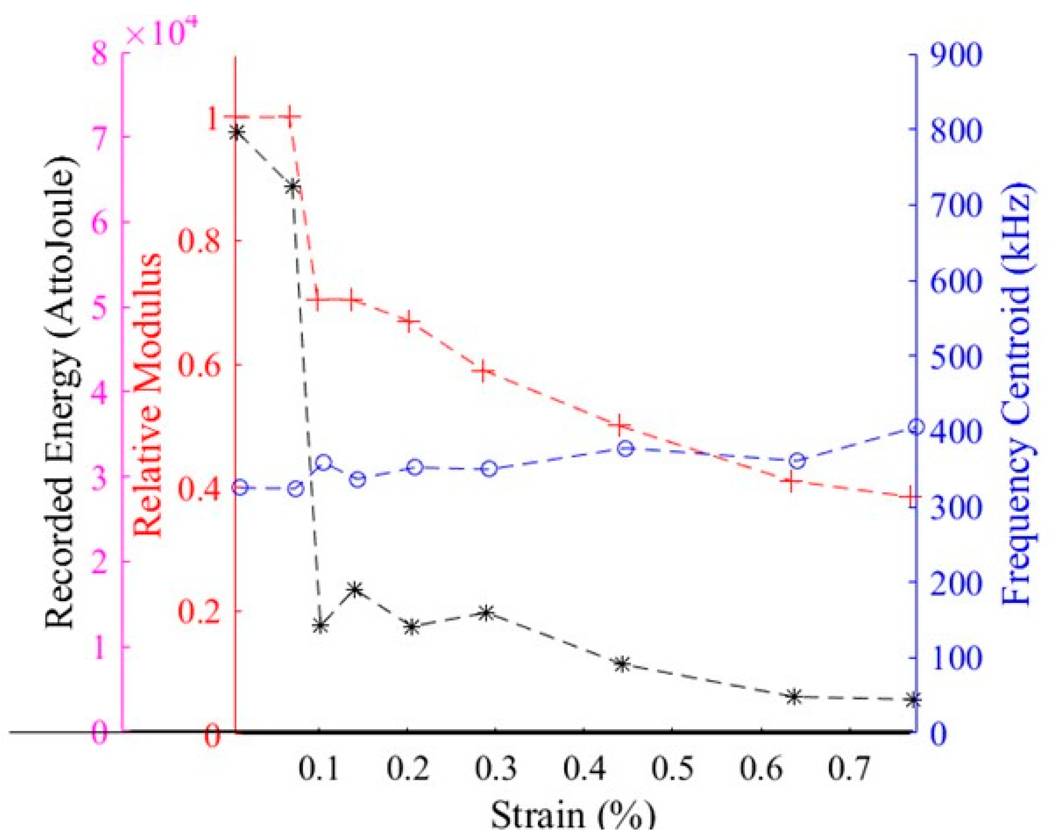
Figure 4 shows the evolution of the recorded energy, the damage index (1 − D) and the frequency centroid as a function of strain during a tensile test of CMC. To describe stiffness loss, the variable D is used, defined through the well-known relation:
where E(t) is the secant elastic modulus at the time t and for the strain ε and E0 is the initial elastic modulus. Around 0.1% a significant decrease in elastic modulus is observed due to matrix multi cracking. Damage in matrix results from cracks located in the interplay matrix, in the transverse tows and in the longitudinal tows. Above 0.6%, the elastic modulus stabilizes due to saturation of matrix cracking. The waveform is a signal with a sweeping in frequency. The signal for the actuator is the same along the test and contains various frequency components from 100 KHz to 950 KHz. The Figure 4 indicates an evolution of the recorded energy with damage, a significant decrease is observed just after matrix cracking. It is shown that waveforms are distorted with damage evolution. The recorded energy is strongly affected. The frequency centroid seems not to be affected by the evolution of damage. The same result is obtained with the average frequency and the peak frequency. This result is very important for the lifetime estimation based on the recorded energy and it shows that it would be necessary to correct the energy or the amplitude accordingly with the damage evolution.
3.2. Influence of the Choice of Sensor
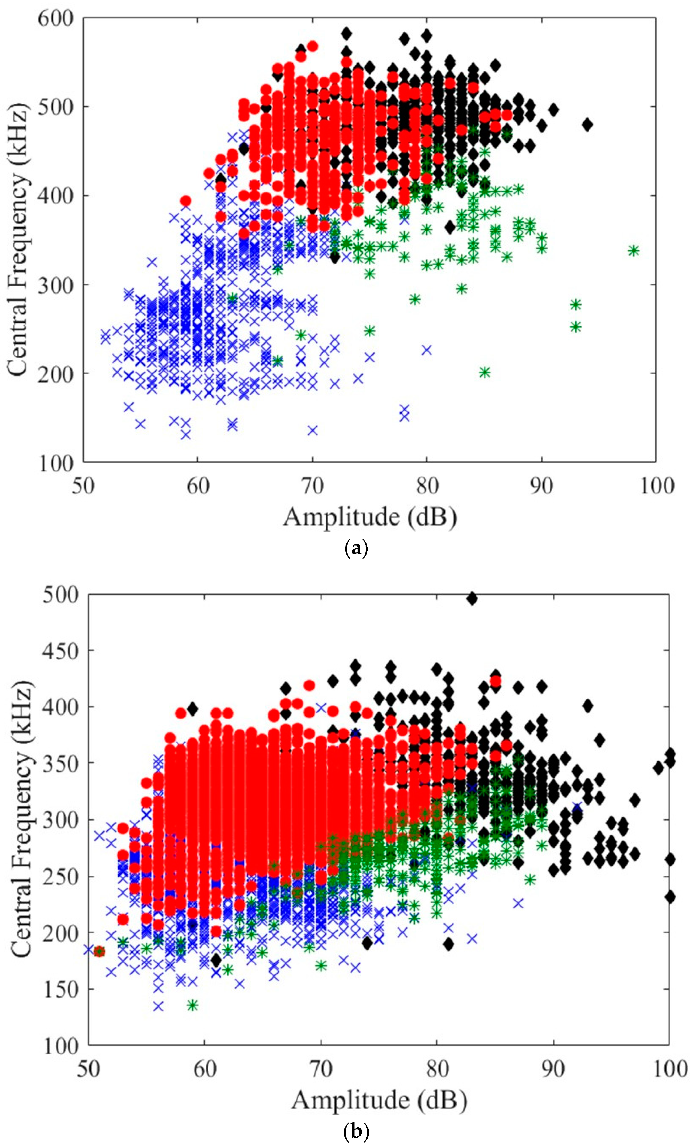
The cumulative AE energy recorded by both sensors, μ80 and PicoHF during tensile tests, is shown in Figure 5 for the vinylester composite. The global behaviour is equivalent in terms of the energy recorded. Nevertheless, we can notice that the μ80 sensors have better signal detection than PicoHF sensors, especially during the first part of the test. In addition to a different sensitivity, the choice of sensor plays an important role in the characteristics of the recorded signals. Figure 6a,b show the whole data population recorded at both sensors in the plane amplitude/frequency barycentre for the signals recorded during a tensile test on glass fibres/PA6.6 polyamide composites and for the glass fibre/vinylester composites. It is clear that the sensor noticeably distorts the AE signals. Table 2 summarizes the mean value and the lower and upper limits for several AE descriptors. In order to check the possibility to structure these data, an unsupervised classification is conducted. The majorities of the descriptors have an exponential distribution, which often makes them incomparable with other descriptors such as amplitude or mean frequency, which have Gaussian distributions. It may be useful to apply a natural logarithm to these “exponential” descriptors, so that their distributions can be approximated using a Gaussian law. The dendrogram allows the choice of the same descriptors (ln(Rise time), Duration, amplitude, ln(energy), FP (frequency peak) and FC (frequency centroid)). According to the DB (Davies and Bouldin) and SI (Silhouette) indices [2,13], the classification lead to a solution with four classes. Figure 7a,b shows the representation of the classes in the plane frequency centroid/amplitude. Figure 8 represents the radar chart for the normalized median values of several classes. The same colour is attributed to the equivalent classes obtained with the two kinds of sensors. The differences in the segmentation is visible. The sensor bandwidth and its sensitivity have a significant influence on the degree of class separation and class characteristics. Moreover, it is difficult to establish a link between the characteristics of the class identified with the two kinds of sensors. The aim of compensating the effect of sensor seems to be difficult. The majority class (Red class) recorded by the sensor μ80 is reduced by 90% with the sensor picoHF. The class with the highest rise time (blue class), second majority class with the sensor μ80 is also drastically reduced with the PicoHF sensor (reduced by 80%). For the most energetic classes (black and green classes), the same number of signals are recorded but the repartition is different. The Black class is the majority energetic class with the μ80 sensor instead of the green class for the picoHF. Even if it is possible to identify an equivalent structuration of data, the correlation with the mechanisms of damage is more complicate with the use of different sensors.
3.3. Influence of the Sensor Position
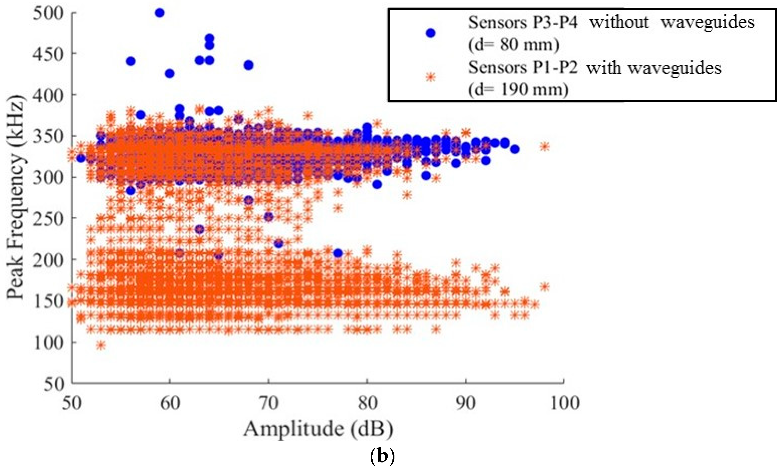
The results presented herein are based on the AE signals located along the gauge length by the two couples of sensors denoted μ80 P1-P2 and μ80 P3-P4 on CMC composites. For the whole number of signals, the median values of the descriptors are calculated. Table 2 shows the median value for the sensor located at P1 and for the sensor at P3. For the configuration comprising the sensors placed directly on the specimen on the 25 calculated descriptors, 17 descriptors display a relative difference greater than 25% between the two acquisition configurations. Overall, the values of descriptors related to time (rise time, duration) are higher for the sensor located in the grips while those descriptors such as energy are lower. A decreasing trend is seen again both for the frequency (Figure 9a). The mean value of the central frequency decreases about 25% and the mean value of the peak frequency decreases about 50%. Peak frequency, which seems to be more relevant with the AU measure, is not suitable to describe the source and could affect the ability to identify damage modes. It is understandable that if a separation distance of 40 mm is responsible for a change in the frequency content more than 25%, one should be very careful in application of any laboratory characterization scheme in a real structure. The effect of the location of the sensor is clearly highlighted here even in the laboratory scale. It can be explained by the nature of the considered acoustic waves, mainly surface waves, probably modified during propagation in the part of the specimen that is affixed to the clamps. This observation emphasizes a little more the importance of understanding the link between the signal received and the source.
In order to compare the descriptors recorded directly on the specimen and at the extremities of the waveguide, a comparison of the data recorded by sensor located at P1 at the end of the waveguide and by sensor P3 at the surface is done. It has shown that 17 descriptors out of 25 have a relative difference greater than 25%. We also note that the rise time, the energy and the frequency mainly the peak frequency are greatly affected by propagation distance. These results show that is difficult to assign a damage mechanism to an AE signal only with the value of the frequency.
3.4. Influence of the Descriptors Selection
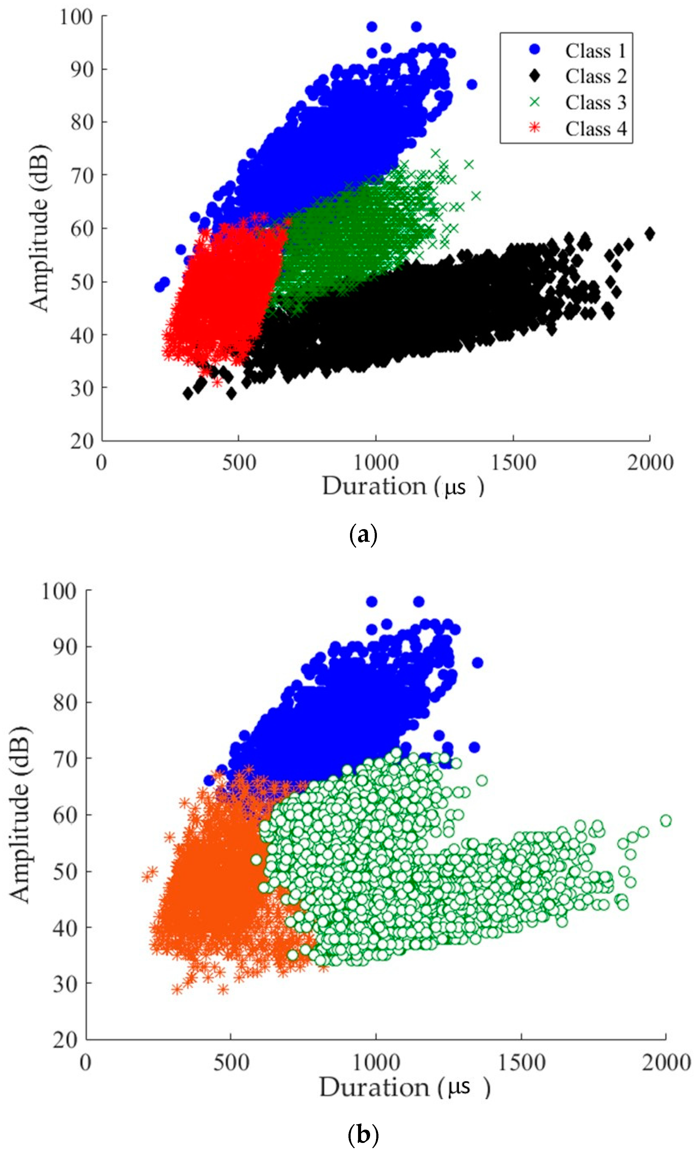
The last part of this section is devoted to the study of the sensitivity of classification algorithms and to the influence of the choice of descriptors on the data segmentation with artificial data sets. This data set is artificially generated from actual acoustic emission data [13]. The data set contains 4 clusters (2000 signals each) that are representative of actual experimental data (Figure 10). This data set, being very similar to real data, will illustrate the notion of relevant descriptor. This data set is initially described by 18 descriptors then by 3 relevant descriptors (amplitude, ln [counts to peak], ln [energy]). The user according to the known structure of the data has defined the relevant parameters. When the 18 descriptors are considered, the best-obtained segmentation is still a 3-cluster solution. Only one cluster is correctly identified with 1985 signals. The average Silhouette for this group is greater than 0.6, while for the other two groups, the average Silhouette is less than 0.5. Considering only the three relevant descriptors (amplitude, ln [counts to peak], ln [energy]), the 4-cluster solution corresponding to the actual data structure is obtained. The four clusters have an average silhouette greater than 0.6 and there are only 120 misclassified signals. In the unsupervised classification, it is impossible for the user to visually determine the relevant parameters from an experimental point of view. The use of the correlation matrix of the 18 descriptors only allows the selection of uncorrelated descriptors and does not give any indication of their relevance.
3.5. Influence of the Sensors Coupling
This protocol developed by Maillet [43] is applied on a test conducted at intermediate temperature and the sensors are located in the grips at the position P1 and P2. The energy distribution function is drawn for the two sensors P1 and P2, for the signals corresponding to the sources located at the beginning of loading in the ±5 mm interval around the centre of the useful zone. This figure shows a significant difference between the two sensors (Figure 11), the distribution functions are not superimposed. If the recorded energy is affected, it goes without saying that several descriptors are affected by this different coupling. This difference is attributed mainly to a difference in coupling between the sensors and the surface of the material due to the applied pressure. In these tests, it is not possible to control the applied pressure on the sensor. This result shows the necessity to control the coupling of the sensors with the material surface.
4. Conclusions
The effect of the sensor, its coupling and the propagation leads to important changes in the AE features used in data classification. Since the waveforms parameters change with sensors or with propagation, the classification boundaries between classes should also be adjusted. It is obvious that the boundaries between several classes depend on the type of sensors and on the distance between the source and the sensor.
The results show that it is necessary to take into account the effect of sensor, of propagation and of damage. This approach based on the clustering is very popular but suffers from a lack of robustness since the identification of the acoustic signature of the several damage modes does not take into account possible variations due to changes in acquisition set-up. The results show that the change in the waveform and in AE features is quite strong in terms of frequency and energy and should not be neglected. The interpretation of an AE signal appears in this particularly difficult context. It is important to differentiate what is characteristic of the source from what comes from transformations related to propagation and acquisition. In order to achieve this objective, the modelling of the entire AE chain from the source to the analysed signal seems indispensable. This quantitative approach to AE relies on the use of modelling techniques in order to evaluate the impact of each transformation step on the signal. This fundamental aspect is essential for the good use of AE data, choice of sensors and needs to be developed in order to make this technique more reliable.
Author Contributions
All the authors have contributed to analysing the data and to writing this paper.
Acknowledgments
The collaboration with SAFRAN Ceramics is gratefully acknowledged for the work on CMC composites.
Conflicts of Interest
The authors declare no conflict of interest.
References
- Sause, M. Situ Monitoring of Fiber-Reinforced Composites: Theory, Basic Concepts, Methods, and Applications; Springer Series in Materials Science; Springer: Berlin, Germany, 2016; Volume 242. [Google Scholar]
- Godin, N.; Reynaud, P.; Fantozzi, G. Acoustic Emission and Durability of Composites Materials; ISTE-Wiley: London, UK, 2018; ISBN 9781786300195. [Google Scholar]
- Romhany, G.; Czigany, T.; Karger-Kocsis, J. Failure assessment and evaluation of damage development and crack growth in polymer composites via localization and acoustic emission events: A review Polymer Reviews. Polym. Rev. 2017, 57, 397–439. [Google Scholar] [CrossRef]
- Morscher, G.N.; Godin, N. Use of Acoustic Emission for Ceramic Matrix Composites; John Wiley&Sons, Inc.: Hoboken, NJ, USA, 2014; pp. 569–590. [Google Scholar]
- Anastassopoulos, A.; Philippidis, T. Clustering methodology for the evaluation of acoustic emission from composites. J. Acoust. Emiss. 1995, 13, 11–12. [Google Scholar]
- Huguet, S.; Godin, N.; Gaertner, R.; Salmon, L.; Villard, D. Use of acoustic emission to identify damages modes in glass fibre reinforced polyester. Compos. Sci. Technol. 2002, 62, 1433–1444. [Google Scholar] [CrossRef]
- Kostopoulos, V.; Loutas, T.; Kontsos, A.; Sotiriadis, G.; Pappas, Y. On the identification of the failure machanisms in oxide/oxide composites using acoustic emission. NDT E Int. 2003, 36, 571–580. [Google Scholar] [CrossRef]
- Maillet, E.; Godin, N.; R’Mili, M.; Reynaud, P.; Lamon, J.; Fantozzi, G. Analysis of Acoustic Emission energy release during static fatigue tests at intermediate temperatures on Ceramic Matrix Composites: Towards rutpure time prediction. Compos. Sci. Technol. 2012, 72, 1001–1007. [Google Scholar] [CrossRef]
- Ramasso, E.; Placet, V.; Boubakar, L. Unsupervised Consensus Clustering of Acoustic Emission Time-Series for Robust Damage Sequence Estimation in Composites. IEEE Trans. Instrum. Meas. 2015, 64, 3297–3307. [Google Scholar] [CrossRef]
- Marec, A.; Thomas, J.-H.; El Guerjouma, R. Damage characterization of polymer-based composite materials: Multivariable analysis and wavelet transform for clustering acoustic emission data. Mech. Syst. Signal Process. 2008, 22, 1441–1464. [Google Scholar] [CrossRef]
- Li, L.; Lomov, S.V.; Yan, X. Correlation of acoustic emission with optically observed damage in a glass/epoxy woven laminate under tensile loading. Compos. Struct. 2015, 123, 45–53. [Google Scholar] [CrossRef]
- Malpot, A.; Touchard, F.; Bergamo, S. An investigation of the influence of moisture on fatigue damage mechanisms in a woven glass-fibre-reinforced PA66 composite using acoustic emission and infrared thermography. Compos. Part B Eng. 2017, 130, 11–20. [Google Scholar] [CrossRef]
- Sibil, A.; Godin, N.; R’Mili, M.; Maillet, E.; Fantozzi, G. Optimization of acoustic emission data clustering by a genetic algorithm method. J. Nondestruct. Eval. 2012, 31, 169–180. [Google Scholar] [CrossRef]
- Godin, N.; Reynaud, P.; R’Mili, M.; Fantozzi, G. Identification of Damage Mechanisms with Acoustic Emission Monitoring: Interests and Limitations; Giovanni Pappalettera, G., Barile, C., Eds.; Nova Science Publishers: Hauppauge, NY, USA, 2017. [Google Scholar]
- Sause, M.; Gribov, A.; Unwin, A.R.; Horn, S. Pattern recognition approach to identify natural clusters of acoustic emission signals. Pattern Recognit. Lett. 2012, 33, 17–23. [Google Scholar] [CrossRef]
- Sause, M.; Horn, S. Simulation of acoustic emission in planar carbon fiber reinforced plastic specimens. J. Nondestr. Eval. 2010, 29, 123–142. [Google Scholar] [CrossRef]
- Sause, M.; Hamstad, M.; Horn, S. Finite element modelling of lamb wave propagation in anisotropic hybrid materials. Compos. Part B 2013, 53, 249–257. [Google Scholar] [CrossRef]
- Ben Khalifa, W.; Jezzine, K.; Hello, G.; Grondel, S. Analytical modelling of acoustic emission from buried or surface-breaking cracks under stress. J. Phys. Conf. Ser. 2012, 353, 012016. [Google Scholar] [CrossRef] [Green Version]
- Le Gall, T.; Godin, N.; Monnier, T.; Fusco, C.; Hamam, Z. Acoustic Emission modeling from the source to the detected signal: Model validation and identification of relevant descriptors. J. Acoust. Emiss. 2016, 34, S59–S64. [Google Scholar]
- Loutas, T.; Eleftheroglou, N.; Zarouchas, D. A data-driven probabilistic framework towards the in-situ prognostics of fatigue life of composites based on acoustic emission data. Compos. Struct. 2017, 161, 522–529. [Google Scholar] [CrossRef]
- Suresh Kumar, C.; Arumugam, V.; Sengottuvelusamy, R.; Srinivasan, S.; Dhakal, H.N. Failure strength prediction of glass/epoxy composite laminates from acoustic emission parameters using artificial neural network. Appl. Acoust. 2017, 115, 32–41. [Google Scholar] [CrossRef]
- Eleftheroglou, N.; Loutas, T. Fatigue damage diagnostics and prognostics of composites utilizing structural health monitoring data and stochastic processes. Struct. Health Monit. 2016, 15, 473–488. [Google Scholar] [CrossRef]
- Arumugam, V.; Shankar, R.; Naren Sridhar, B.T.N.; Joseph Stanley, A. Ultimate Strength Prediction of Carbon/Epoxy Tensile Specimens from Acoustic Emission Data. J. Mater. Sci. Technol. 2010, 26, 725–729. [Google Scholar] [CrossRef]
- Sasikumar, T.; Rajendraboopathy, S.; Usha, K.M.; Vasudev, E.S. Failure strength prediction of unidirectional tensile coupons using acoustic emission peak amplitude and energy parameter with artificial neural networks. Compos. Sci. Technol. 2009, 69, 1151–1155. [Google Scholar] [CrossRef]
- Momon, S.; Moevus, M.; Godin, N.; R’Mili, M.; Reynaud, P.; Fantozzi, G.; Fayolle, G. Acoustic emission and lifetime prediction during static fatigue tests on ceramic matrix composite at high temperature under air. Compos. Part A 2010, 41, 913–918. [Google Scholar] [CrossRef]
- Racle, E.; Godin, N.; Reynaud, P.; Fantozzi, G. Fatigue Lifetime of Ceramic Matrix Composites at Intermediate Temperature by Acoustic Emission. Materials 2017, 10, 658. [Google Scholar] [CrossRef] [PubMed]
- Gorman, M.R. Plate wave acoustic emission. J. Acoust. Soc. Am. 1991, 90, 358–364. [Google Scholar] [CrossRef]
- Gorman, M.R.; Ziola, S. Plate waves produced by transfert matrix cracking. Ultrasonics 1991, 29, 245–251. [Google Scholar] [CrossRef]
- Gorman, M.R. Some corrections between AE testing of large structures and small samples. Nondestruct. Test. Eval. 1998, 14, 89–104. [Google Scholar] [CrossRef]
- Aggelis, D.G.; Shiotani, T.; Papacharalampopoulos, A.; Polyzos, D. The Influence of propagation path on elastic waves as measured by acoustic emission parameters. Struct. Health Monit. 2011, 11, 359–366. [Google Scholar] [CrossRef]
- Aggelis, D.G.; Matikas, T. Effect of plate wave dispersion on the acoustic emission parameters in metals. Comput. Struct. 2012, 98, 17–22. [Google Scholar] [CrossRef]
- Hamstad, M.A.; Downs, K.S. On characterization and location of acoustic emission sources in real size composite structures—A waveform study. J. Acoust. Emiss. 1995, 13, 31–41. [Google Scholar]
- Hamstad, M.A.; O’Gallagher, A.; Gary, J.A. wavelet transform applied to acoustic emission signals: Part 1: Source identification. J. Acoust. Emiss. 2002, 20, 39–61. [Google Scholar]
- Kharrat, M.; Placet, V.; Ramasso, E.; Boubakar, L. Influence of damage accumulation under fatigue loading on the AE-based health assessment of composite material: Wave distortion and AE-features evolution as a function of damage level. Compos. Part A Appl. Sci. Manuf. 2018, 109, 615–627. [Google Scholar] [CrossRef]
- Carpinteri, A.; Lacidogna, G.; Accornero, F.; Mpalaskas, A.C.; Matikas, T.E.; Aggelis, D.G. Influence of damage in the acoustic emission parameters. Cem. Concr. Compos. 2013, 44, 9–16. [Google Scholar] [CrossRef]
- Maillet, E.; Baker, C.; Morscher, G.N.; Pujar Vijay, V.; Lemanski, J.R. Feasibility and limitations of damage identification in composite materials using acoustic emission. Compos. Part A 2015, 75, 77–83. [Google Scholar] [CrossRef]
- Maillet, E.; Godin, N.; R’Mili, M.; Reynaud, P.; Fantozzi, G.; Lamon, J. Damage monitoring and identification in SiC/SiC minicomposites using combined acousto-ultrasonics and acoustic emission. Compos. Part A 2014, 57, 8–15. [Google Scholar] [CrossRef]
- Hatano, H.; Mori, E. Acoustic-emission transducer and its absolute calibration. J. Acoust. Soc. Am. 1976, 59, 344–349. [Google Scholar] [CrossRef]
- Dia, S.; Monnier, T.; Godin, N.; Zhang, F. Primary Calibration of Acoustic Emission Sensors by the Method of Reciprocity, Theoretical and Experimental Considerations. J. Acoust. Emiss. 2012, 30, 152–166. [Google Scholar]
- Goujon, L.; Baboux, J.C. Behaviour of acoustic emission sensors using broadband calibration techniques. Meas. Sci. Technol. 2003, 14, 903–908. [Google Scholar] [CrossRef]
- McLaskey, G.C.; Glaser, S.D. Acoustic Emission Sensor Calibration for Absolute Source Measurements. J. Nondestruct. Eval. 2012, 31, 157–168. [Google Scholar] [CrossRef]
- Moevus, M.; Godin, N.; R’Mili, M.; Rouby, D.; Reynaud, P.; Fantozzi, G.; Fayolle, G. Analyse of damage mechanisms and associated acoustic emission in two SiC/[Si-B-C] composites exhibiting different tensile curves. Part II: Unsupervised acoustic emission data clustering. Compos. Sci. Technol. 2008, 68, 1258–1265. [Google Scholar] [CrossRef]
- Maillet, E.; Godin, N.; R'Mili, M.; Reynaud, P.; Fantozzi, G.; Lamon, J. Real-time evaluation of energy attenuation: A novel approach to acoustic emission analysis for damage monitoring of ceramic matrix composites. J. Eur. Ceram. Soc. 2014, 34, 1673–1679. [Google Scholar] [CrossRef]
- Theobald, P.; Zeqiri, B.; Avison, J. Couplants and their influence on AE sensor sensitivity. J. Acoust. Emiss. 2008, 26, 91–97. [Google Scholar]
- Ono, K. Through-Transmission Characteristics of AE Sensor Couplants. J. Acoust. Emiss. 2017, 34, 1–11. [Google Scholar]
Figure 1.
Schematic diagram of an instrumented specimen with four sensors, (a) on ceramic matrix composites (CMC) samples without a waveguide (b) on CMC samples with a waveguide.
Figure 1.
Schematic diagram of an instrumented specimen with four sensors, (a) on ceramic matrix composites (CMC) samples without a waveguide (b) on CMC samples with a waveguide.

Figure 2.
Calibration curve with the reciprocity method. Sensibility in reception for a sensor μ80 on steel material for the Rayleigh waves.
Figure 2.
Calibration curve with the reciprocity method. Sensibility in reception for a sensor μ80 on steel material for the Rayleigh waves.

Figure 3.
(a) Amplitude and frequency recorded by a μ80 sensor for signals of different frequencies and same energy generated by an acousto-ultrasonic card. (× Weighted Frequency, * Peak Frequency, + Central Frequency and ◊ Average Frequency) (b) PPi versus input frequency. (The input signal is generated with a specific frequency equal to 150 kHz up to 950 kHz, amplitude 5 volts and rise time 20 μs. (Propagation distance of 100 mm, composite material propagation medium with undamaged SiCf/SiC, actuator μ80 sensor).


Figure 4.
Evolution of the recorded acoustic energy, the frequency centroid and the relative modulus versus strain for a tensile test on CMC at room temperature. (The input signal is generated with a frequency in the range of 150 kHz and 950 kHz, amplitude 5 volts and rise time 20 μs, actuator μ80 sensor).

Figure 5.
Stress-strain curve and the cumulated recorded energy during a tensile test on glass fibres/vinylester matrix monitored with two types of sensors (μ80 and pico HF) located at the same place on the gauge length on each face.
Figure 5.
Stress-strain curve and the cumulated recorded energy during a tensile test on glass fibres/vinylester matrix monitored with two types of sensors (μ80 and pico HF) located at the same place on the gauge length on each face.

Figure 6.
Frequency centroid versus amplitude for the signals recorded during a tensile test with two types of sensors μ80 and pico HF located on the gauge length at the same place (a) Glass fibres/polyamide 6.6 matrix and (b) glass fibres/vinylester matrix.
Figure 6.
Frequency centroid versus amplitude for the signals recorded during a tensile test with two types of sensors μ80 and pico HF located on the gauge length at the same place (a) Glass fibres/polyamide 6.6 matrix and (b) glass fibres/vinylester matrix.

Figure 7.
Results of the classification in the plane Frequency Centroid/Amplitude for the data recorded during tensile tests of glass fibre/Vinylester composites (a) data recorded with the pico HF sensors and (b) with the μ80 sensors. (For the classification, the selected descriptors are Rise time, Duration, amplitude, energy, FP (frequency peak) and FC (frequency centroid)).

Figure 8.
Radar chart for the four classes obtained with the two kinds of sensors for the data recorded during tensile tests of glass fibre/Vinylester composites (a) μ80 sensor and (b) picoHF sensor (class blue: highest rise time, Black class: Highest energy, green class: second class in energy term, red class: the last one class) (E energy, RT rise time, D duration, A amplitude, RA rise angle, AF average frequency and FC frequency centroid).

Figure 9.
(a) Frequency centroid versus amplitude for the data collected during a tensile test on CMC composite with four similar sensors applied on the surface of the specimen (b) Peak Frequency versus amplitude for the signals located along the gauge length during a tensile test on CMC composite, data recorded with and without waveguides.


Figure 10.
(a) Initial dataset with four artificial classes (b) results of the segmentation, accordingly to the DB (Davies and Bouldin) and SI (Silhouette) indices, with the 18 descriptors selected.
Figure 10.
(a) Initial dataset with four artificial classes (b) results of the segmentation, accordingly to the DB (Davies and Bouldin) and SI (Silhouette) indices, with the 18 descriptors selected.

Figure 11.
Energy cumulative distribution functions for a fatigue tests at 450 °C on CMC composite (±5 mm interval around the middle of the gauge length for strain lower than 0.1%).
Figure 11.
Energy cumulative distribution functions for a fatigue tests at 450 °C on CMC composite (±5 mm interval around the middle of the gauge length for strain lower than 0.1%).


Table 1.
Descriptors set of acoustic emission (AE) signals.
| Descriptor | Symbol | Unit |
|---|---|---|
| Rise time | RT | µs |
| Counts | C | - |
| Duration | D | µs |
| Amplitude | A | dB |
| Average Frequency | AF | kHz |
| Counts to peak | CP | - |
| Decay frequency | DF | kHz |
| Rise frequency | RF | kHz |
| Absolute energy | E | attoJ |
| Frequency central | FC | kHz |
| Peak Frequency | FP | kHz |
| Rise time/duration | RT/D | - |
| Duration/Amplitude | D/A | µs/dB |
| Decay time | D-RT | µs |
| Rise angle | RA = A/RT | dB/µs |
| Decay angle | A/(D-RT) | dB/µs |
| Rise time/Decay time | RT/(D-RT) | - |
| Relative energy | E/A | attoJ/dB |
| Counts to peak/Counts | CP/C | - |
| Amplitude/Frequency | A/AF | dB/kHz |
| Weighted Frequency | WF | kHz |
| Partial Power 1 [100–200 kHz] | PP1 | % |
| Partial Power 2 [200–400 kHz] | PP2 | % |
| Partial Power 3 [400–600 kHz] | PP3 | % |
| Partial Power 4 [600–1000 kHz] | PP4 | % |
Table 2.
Median values, the upper and the lower quartiles for several descriptors recorded during tensile test on composite glass fibres and vinylester matrix with two types of sensors located at the same place (micro80 and picoHF) and during tensile test on CMC composite with μ80 sensors located at P1 and P3 on the surface of the specimen.
| Descriptor | Tensile Test on Composite Glass Fibres and Vinylester Matrix with Two Kind of Sensors (micro80 and picoHF) | Tensile Test on CMC Composite with μ80 Sensors Located at P1 and P3 on the Surface of the Specimen | ||||
|---|---|---|---|---|---|---|
| Rise Time (μs) | Sensor | Micro80 | PicoHF | Sensor | Micro80 P1 | Micro80 P3 |
| Q1 | 7 | 6 | Q1 | 21 | 6 | |
| Median value | 12 | 11 | Median value | 33 | 15 | |
| Q2 | 18 | 15 | Q2 | 50 | 35 | |
| Amplitude (dB) | Sensor | Micro80 | PicoHF | Sensor | Micro80 P1 | Micro80 P3 |
| Q1 | 70 | 70 | Q1 | 50 | 57 | |
| Median value | 77 | 78 | Median value | 57 | 63 | |
| Q2 | 83 | 82 | Q2 | 63 | 72 | |
| Energy (Attojoule) | Sensor | Micro80 | PicoHF | Sensor | Micro80 P1 | Micro80 P3 |
| Q1 | 8352 | 6629 | Q1 | 150 | 550 | |
| Median value | 25,482 | 18,293 | Median value | 591 | 2857 | |
| Q2 | 77,260 | 40,380 | Q2 | 3424 | 13,962 | |
| Amplitude/average Frequency | Sensor | Micro80 | PicoHF | Sensor | Micro80 P1 | Micro80 P3 |
| Q1 | 0.44 | 0.32 | Q1 | 0.24 | 0.27 | |
| Median value | 0.56 | 0.39 | Median value | 0.27 | 0.30 | |
| Q2 | 0.68 | 0.47 | Q2 | 0.30 | 0.33 | |
| Rise angle (dB/μs) | Sensor | Micro80 | PicoHF | Sensor | Micro80 P1 | Micro80 P3 |
| Q1 | 4.26 | 5.18 | Q1 | 0.96 | 1.9 | |
| Median value | 6.82 | 7.22 | Median value | 1.48 | 4.22 | |
| Q2 | 11 | 12 | Q2 | 2.20 | 7.78 | |
| FC (kHz) | Sensor | Micro80 | PicoHF | Sensor | Micro80 P1 | Micro80 P3 |
| Q1 | 279 | 401 | Q1 | 230 | 316 | |
| Median value | 306 | 464 | Median value | 243 | 324 | |
| Q2 | 334 | 487 | Q2 | 254 | 358 | |
| PF (kHz) | Sensor | Micro80 | PicoHF | Sensor | Micro80 P1 | Micro80 P3 |
| Q1 | 232 | 541 | Q1 | 150 | 318 | |
| Median value | 244 | 578 | Median value | 156 | 324 | |
| Q2 | 326 | 593 | Q2 | 205 | 336 | |
| Weighted frequency (kHz) | Sensor | Micro80 | PicoHF | Sensor | Micro80 P1 | Micro80 P3 |
| Q1 | 232 | 541 | Q1 | 190 | 318 | |
| Median value | 286 | 516 | Median value | 201 | 323 | |
| Q2 | 313 | 536 | Q2 | 249 | 328 | |
© 2018 by the authors. Licensee MDPI, Basel, Switzerland. This article is an open access article distributed under the terms and conditions of the Creative Commons Attribution (CC BY) license (http://creativecommons.org/licenses/by/4.0/).
Share and Cite
MDPI and ACS Style
Godin, N.; Reynaud, P.; Fantozzi, G. Challenges and Limitations in the Identification of Acoustic Emission Signature of Damage Mechanisms in Composites Materials. Appl. Sci. 2018, 8, 1267. https://doi.org/10.3390/app8081267
AMA Style
Godin N, Reynaud P, Fantozzi G. Challenges and Limitations in the Identification of Acoustic Emission Signature of Damage Mechanisms in Composites Materials. Applied Sciences. 2018; 8(8):1267. https://doi.org/10.3390/app8081267
Chicago/Turabian StyleGodin, Nathalie, Pascal Reynaud, and Gilbert Fantozzi. 2018. "Challenges and Limitations in the Identification of Acoustic Emission Signature of Damage Mechanisms in Composites Materials" Applied Sciences 8, no. 8: 1267. https://doi.org/10.3390/app8081267
Note that from the first issue of 2016, this journal uses article numbers instead of page numbers. See further details here.