Learning-Based Colorization of Grayscale Aerial Images Using Random Forest Regression


1
Department of Advanced Technology Fusion, Konkuk University, Seoul 05029, Korea
2
Department of Civil and Environmental Engineering, Seoul National University, Seoul 08826, Korea
3
Department of Technology Fusion Engineering, Konkuk University, Seoul 05029, Korea
4
Agency for Defense Development, Daejeon 34060, Korea
*
Author to whom correspondence should be addressed.
Appl. Sci. 2018, 8(8), 1269; https://doi.org/10.3390/app8081269
Submission received: 18 April 2018
/
Revised: 10 July 2018
/
Accepted: 27 July 2018
/
Published: 31 July 2018
(This article belongs to the Special Issue Machine Learning Techniques Applied to Geoscience Information System and Remote Sensing)
Abstract
:Image colorization assigns colors to a grayscale image, which is an important yet difficult image-processing task encountered in various applications. In particular, grayscale aerial image colorization is a poorly posed problem that is affected by the sun elevation angle, seasons, sensor parameters, etc. Furthermore, since different colors may have the same intensity, it is difficult to solve this problem using traditional methods. This study proposes a novel method for the colorization of grayscale aerial images using random forest (RF) regression. The algorithm uses one grayscale image for input and one-color image for reference, both of which have similar seasonal features at the same location. The reference color image is then converted from the Red-Green-Blue (RGB) color space to the CIE L*a*b (Lab) color space in which the luminance is used to extract training pixels; this is done by performing change detection with the input grayscale image, and color information is used to establish color relationships. The proposed method directly establishes color relationships between features of the input grayscale image and color information of the reference color image based on the corresponding training pixels. The experimental results show that the proposed method outperforms several state-of-the-art algorithms in terms of both visual inspection and quantitative evaluation.
1. Introduction
Image colorization can be described as the process of assigning colors to the pixels of a grayscale image in order to increase the image’s visual appeal [1]. This application is often utilized in the image processing community to colorize old grayscale images or movies [2]. Particularly in aerial and satellite imagery, the problem with colorization occurs in a multitude of scenarios that seek to replace topographic maps with vivid, photorealistic renderings of terrain models [3]. There are three main reasons for colorizing aerial and satellite images: (1) grayscale satellite images are available at higher spatial resolutions than their color counterparts are; (2) there are many old grayscale aerial and satellite images that should be represented by color images, typically for monitoring purposes; and (3) grayscale aerial–satellite images can be obtained for approximately one-tenth the cost of color images of the same resolution [3].
In the case of satellite images, modern systems acquire a panchromatic (grayscale) image, with high spatial and low spectral resolutions, and a multispectral (color) image that has complementary properties [4]. In other words, grayscale and color images with different resolutions over the same time period are provided. In order to perform colorization through the color information of the multispectral image while maintaining the high resolution of the panchromatic image, the two components are fused, which is called pansharpening [5]. The fused images provide increased interpretation capabilities and more reliable results [6]. However, this colorization method is confined to satellite images that provide panchromatic and multispectral images of the same time periods, making this type of colorization of aerial images impossible.
On the other hand, grayscale aerial image colorization is a poorly posed problem with more than one solution [7]. As mentioned above, the satellite images fuse the grayscale and color images from the same time period to perform colorization, whereas aerial images do not usually have the two types of imagery available. Furthermore, in contrast to the natural images, this colorization solution depends on the sun elevation angle, season, sensor parameters, etc. It is also problematic that the same intensity may represent different colors, so there is no exact solution [8]. In general, existing colorization methods can be divided into three main categories, all of which have limitations: user-scribbled methods, example-based methods, and those that employ a large number of training images [9]. User-scribbled techniques [10,11,12,13] require a user to manually add colored marks to a grayscale image [13]. The colors from these marks are then smoothly propagated across the entire image, based on an optimization framework. A key weakness is that such methods require users to provide a considerable number of scribbles on the grayscale image, which is time-consuming and requires expertise [14]. Moreover, it is almost impossible to add such markings to large volumes (gigabytes) of aerial imagery. In the case of the example-based method [1,8,9,14,15,16], it typically transfers the color information from a similar reference image to the input grayscale image rather than obtaining chromatic values from the user, thereby reducing the burden on users. However, as feature matching is critical to the quality of the results, satisfactory results cannot be obtained if feature matching is not performed correctly [15]. Moreover, the procedure is very sensitive to image brightness and contrast, whereas real aerial images always include large areas of shadow and low contrast, due to relief, vignetting, and so on. An alternative approach is to employ a large number of training images [17,18,19], which is a recent example of deep learning. These methods use multiple color images to automatically transfer the color information to the grayscale image, and deep neural networks are used to solve the colorization problem. A large database of color images comprising all kinds of objects is used for training the neural networks. The trained model can then be used to efficiently colorize grayscale images. However, this approach is computationally expensive, and the training is significantly slow [15].
In order to overcome these limitations, this study presents a new, fast learning-based technique for the colorization of grayscale aerial images that colorizes them without any user intervention. The algorithm uses one grayscale image as the input and one-color image for reference, both of which have similar seasonal features at the same location. Then, the reference color image is converted from the Red-Green-Blue (RGB) color space to a CIE L*a*b (Lab) color space in which luminance and two-dimensional (2D) color information are stored. Change detection between the input grayscale image and the luminance of the reference color image is performed, and the unchanged region is selected as training pixels, which allows for the extraction of meaningful training data. For colorization, the relationships are established through learning between features of the input grayscale image and the 2D color information of the reference color image based on training pixels. In other words, for the corresponding unchanged region, the color relationships between the two images are directly established, and the colors for the changed region are predicted. At this time, the study’s main technical framework is random forest (RF) regression. Random forest is a data-mining method that has some advantages over most statistical modeling methods [20], including: the ability to model highly nonlinear dimensional relationships; resistance to overfitting; relative robustness with respect to the presence of noise in the data; and the capacity to determine the relevance of the variables used.
The main contributions of this paper can be summarized as follows: (1) to the best of our knowledge, this is the first work that exploits RF regression for aerial imagery colorization, although it has been used for natural image colorization [21,22,23]; (2) this paper develops a novel algorithm that establishes color relationships based on unchanged regions, which predict the color values of the changed regions; (3) this paper establishes color relationships by directly mapping the features of the input grayscale image with the color information of the reference color image; and (4) this paper performs visual and quantitative analyses that show that our method outperforms the current state-of-the-art methods. The rest of this paper is organized as follows. Section 2 describes the materials used in detail, the background of RF regression, and the proposed algorithm. Section 3 presents the colorization results and a detailed comparison with other state-of-the-art colorization algorithms. Section 4 presents the conclusions of the study.
2. Materials and Methods
2.1. Study Site and Data
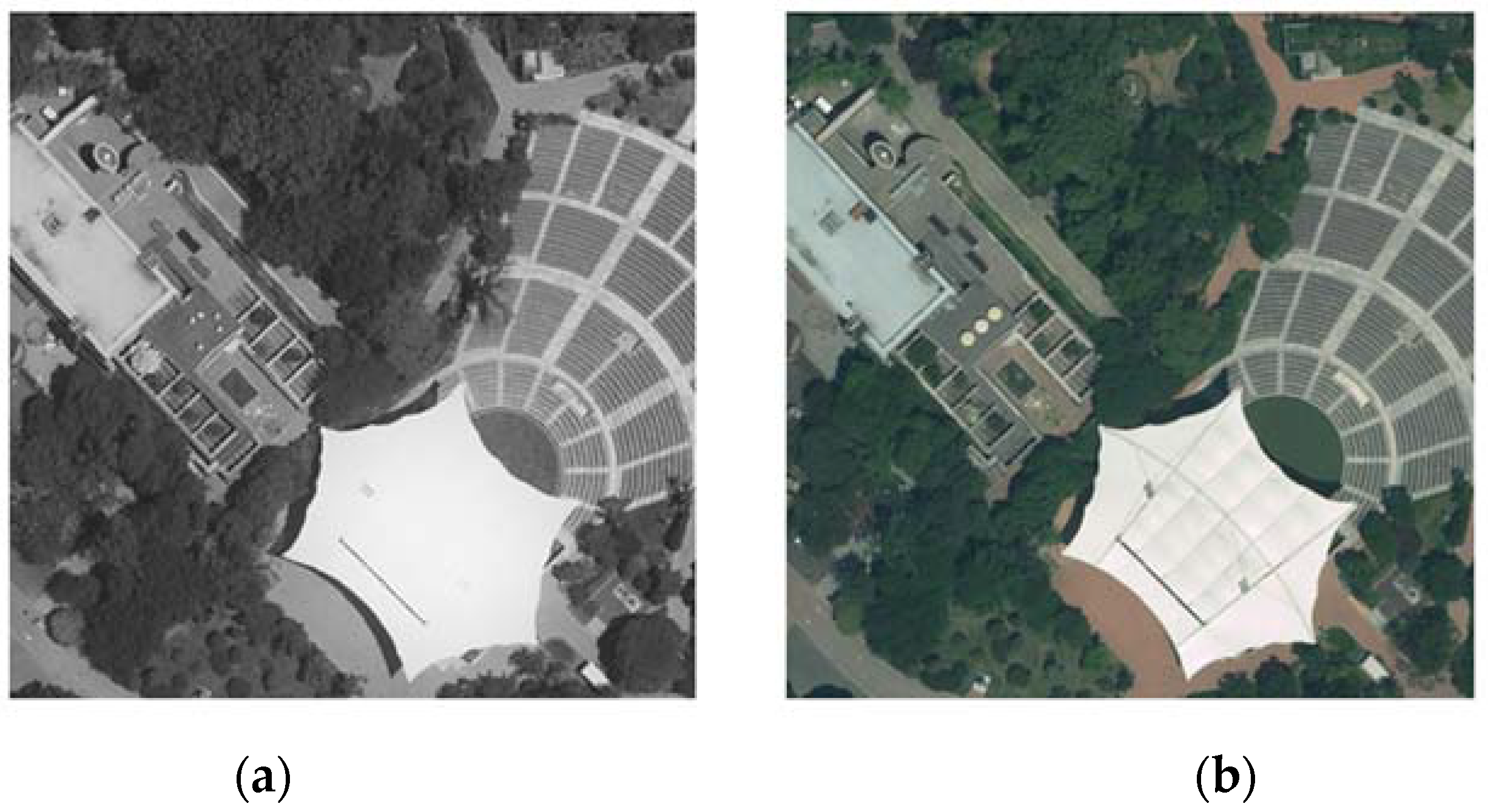
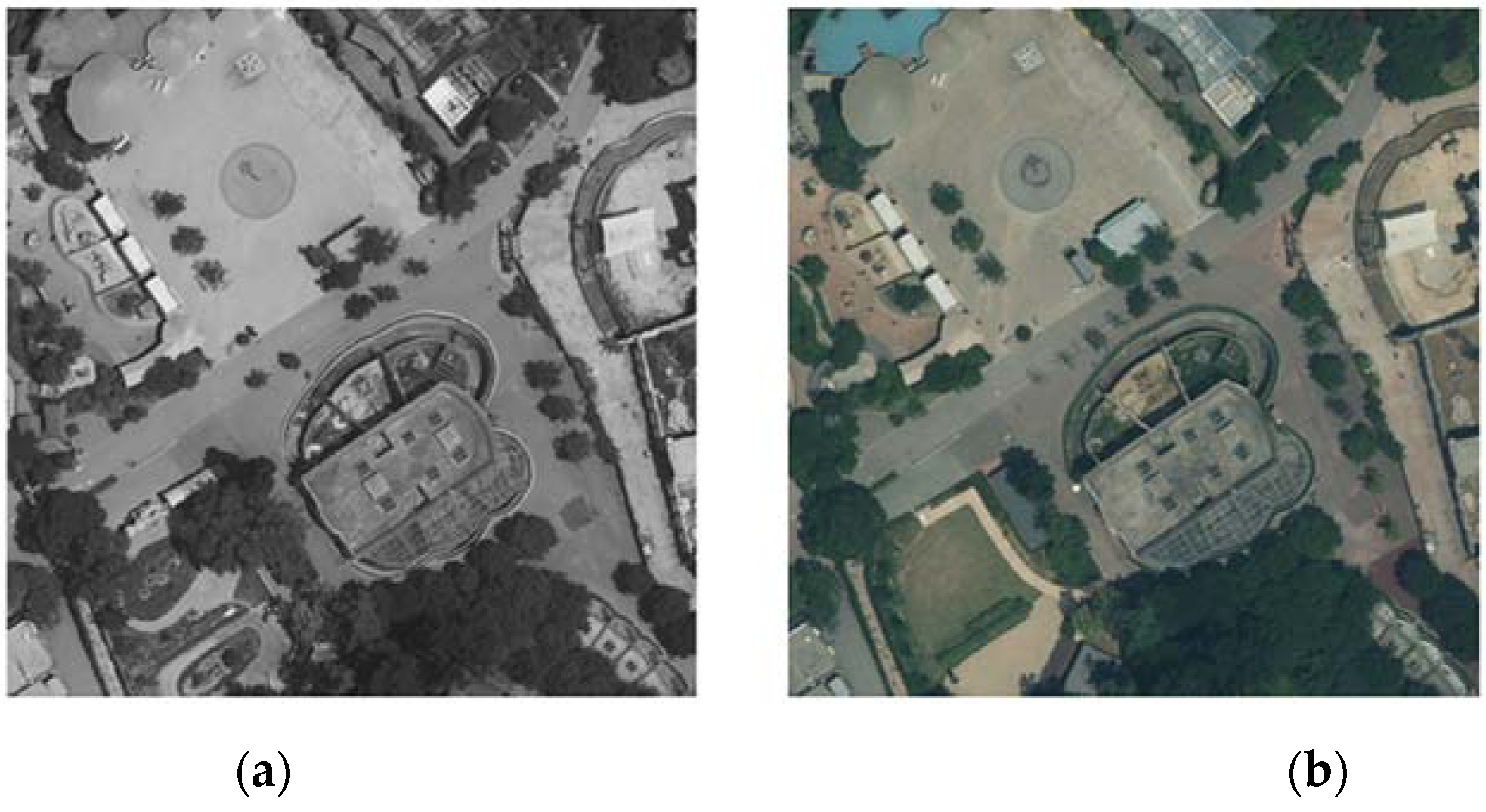
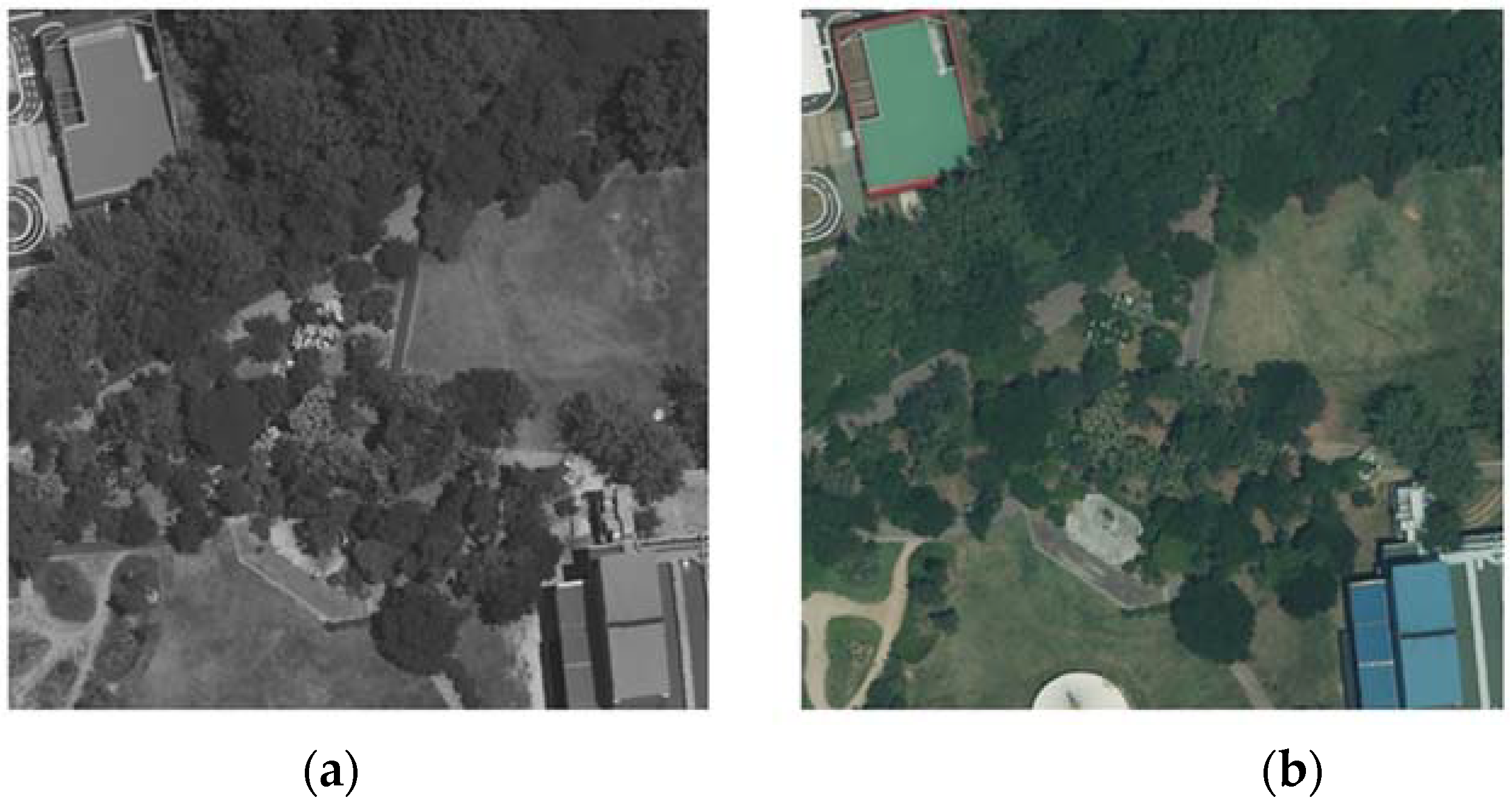
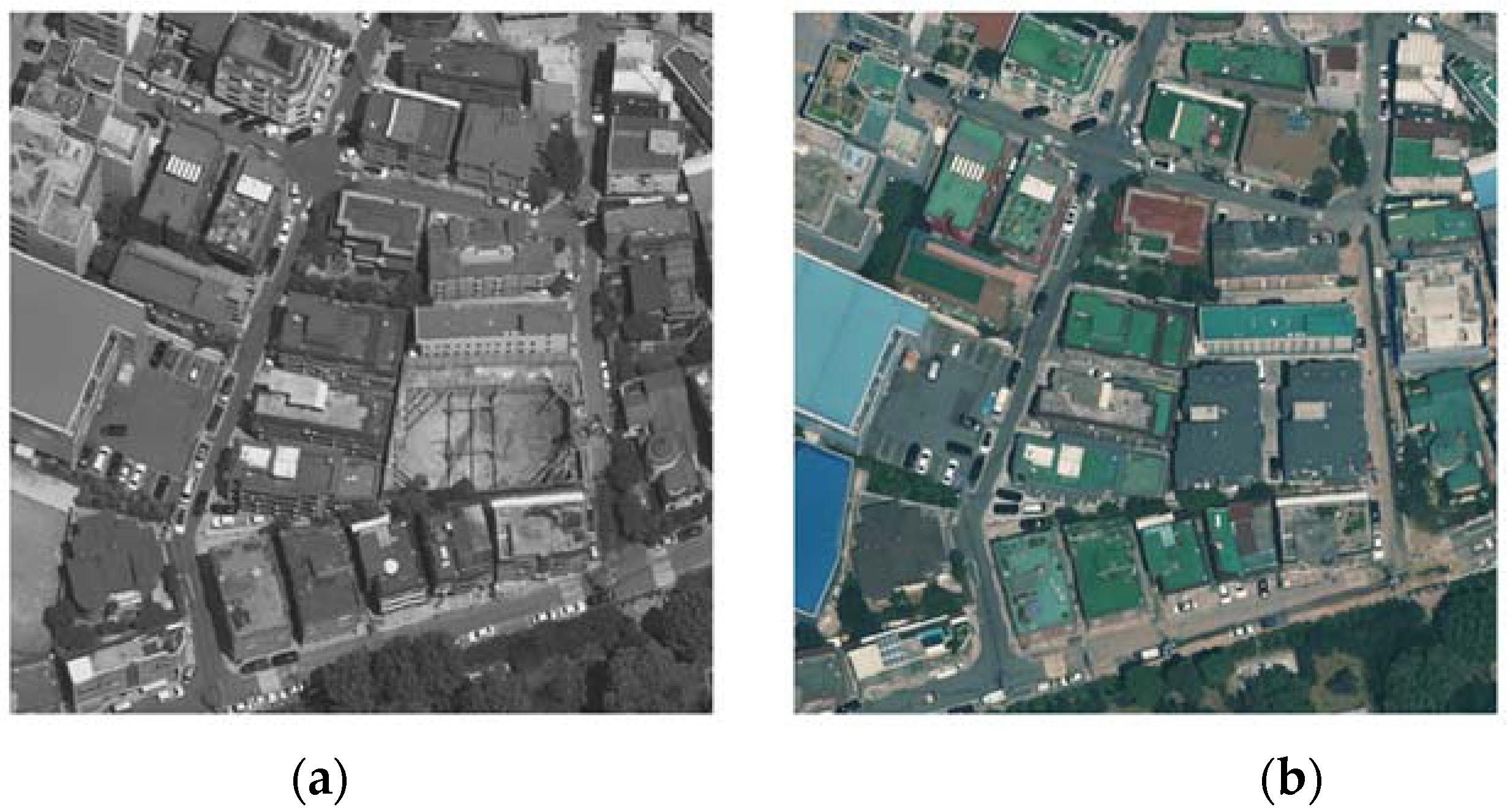
The study sites are located in Gwangjin-gu, in the central–western part of South Korea. The input grayscale images were acquired on 10 June 2013, and the reference color images were acquired on 2 June 2016; both are aerial images at 1 m resolution. Coordinate definition and geometric correction were performed on the images using Environment for Visualizing Images (ENVI) geospatial analytical software (version 4.7, HARRIS Geospatial Solutions, Broomfield, CO, USA). The coordinate system of each image was projected as World Geodetic System (WGS) 84 Universal Transverse Mercator Coordinate System (UTM) 52N, and 30 Ground Control Points (GCPs) were selected for image registration. The 30 GCPs returned a total root mean square error of 0.4970, satisfying values within 0.5 m. Then, based on these GCPs, image registration was performed using the “Warp from GCPs: Image to Image” tool in ENVI. Finally, to achieve reasonable computational time, only a portion of the image was extracted prior to conducting the experiments, which was selected to be 1200 × 1200 pixels. A total of four sites were extracted and are shown in Figure 1, Figure 2, Figure 3 and Figure 4.
2.2. Random Forest
Random forest is a highly versatile ensemble of decision trees that performs well for linear and non-linear prediction by finding a balance between bias and variance [20]. This ensemble learning method constructs and subsequently averages a large number of decision trees for classification or regression purposes [24,25]. At this time, to avoid correlation among the trees, RF increases the diversity of the trees by forcing them to grow from different training data created through a procedure called bootstrap aggregating (bagging) [26]. Bagging refers to aggregating base learners trained through bootstrapping, which creates training data subsets by randomly resampling a given original dataset [27]. That is, as a process of de-correlating trees to train different datasets, it increases stability and makes it more robust when facing slight variations in the input data [28]. Furthermore, approximately one-third of the samples are excluded for the tree training in the bagging process, which is known as the “out-of-bags” (OOB) samples. These OOB samples can be used to evaluate performance, which allows the RF to compute an unbiased estimation of the generalization error without using an external data subset [29]. From the predictions of the OOB samples for every tree in the forest, the mean square error (MSE) is calculated, and the overall MSE is obtained by aggregation, as shown in Equation (1):
where n is the number of trees, yi denotes the prediction for the ith observation, and denotes the average of the OOB predictions for the ith observation.
Furthermore, the use of RF requires the specification of two standard parameters: the number of variables to be selected and tested for the best split at each node (mtry), and the number of trees to be grown (ntree). At each node per tree, the number of mtry variables from the total variables in the model is selected at random, the variable that best splits the input space and the corresponding split are computed, and the input space is split at this point [30]. In a regression problem, the standard value for mtry is one-third of the total number of variables due to computational benefits [31,32]. In the case of ntree, the majority of the studies set the ntree value to 500 since the errors are stabilized before this number of regression trees is achieved [33]. However, recent studies have found that the number of trees does not significantly affect performance improvement, which allows the selection of ntree to consider the performance and training time together [34,35,36].
Random forest can also be used to assess the importance of each variable during modeling. To determine the importance of input variables, a variable is randomly permuted, and regression trees are grown on the modified dataset. The measure of each variable’s importance is then calculated as the difference in the MSE between the original OOB dataset and the modified dataset [37,38]. A key advantage of RF variable importance is that it not only deals with the impact of each variable individually but also looks at multivariate interactions with other variables [39].
2.3. Method
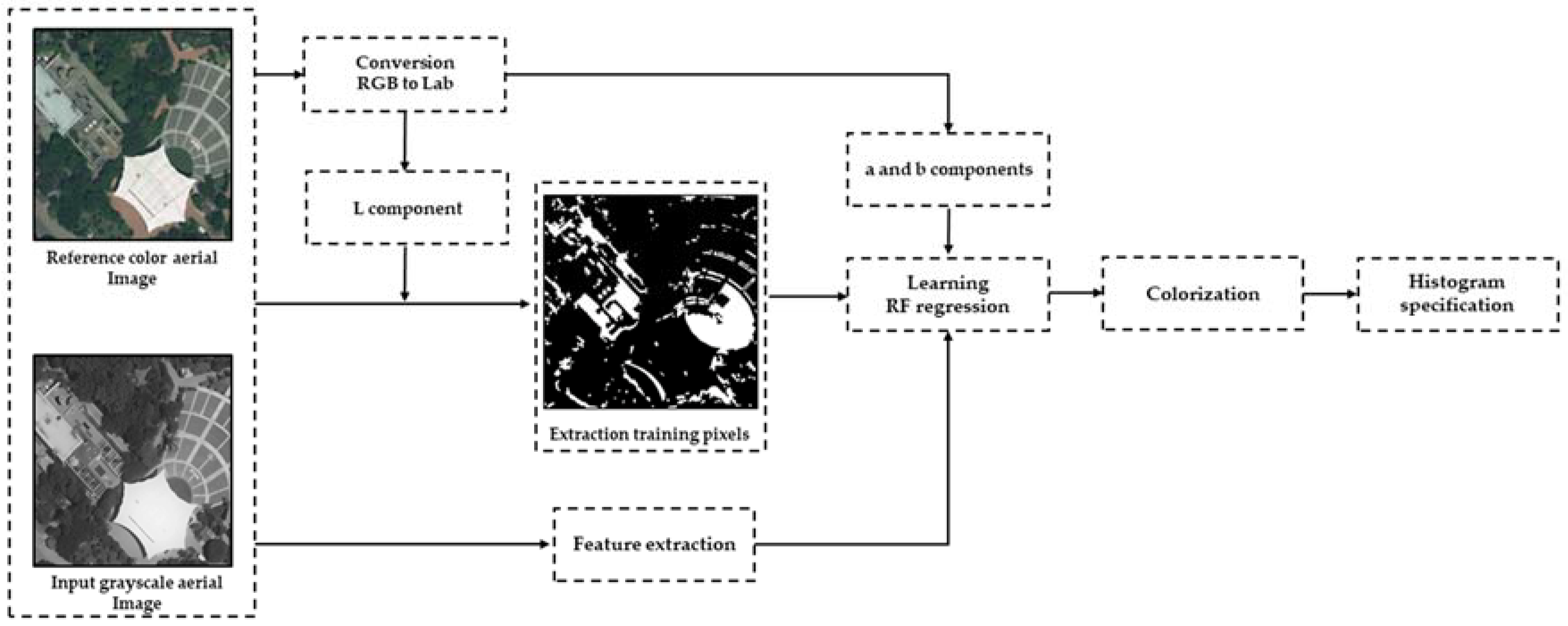
The proposed colorization framework can be decomposed into four steps: (1) pre-processing, (2) feature extraction, (3) colorization, and (4) post-processing, all of which are shown in Figure 5. The first step is to convert the color space and to select the pixels to be used in training for colorization. The second step is to extract feature descriptors of the input grayscale image to be used in learning for color prediction. In the third step, color relationships are established through the proposed method, and colorization is performed on the input grayscale image. The fourth step improves the colorization result by adjusting the histogram. Each of these steps is described below.
2.3.1. Preprocessing
As mentioned above, the proposed preprocessing step is divided into color-space conversion and extraction of training pixels. First, in this study, a Lab color space is selected since its underlying metric has been designed to express color coherency. Furthermore, Lab has three coordinates: L is the luminance, or lightness, which consequently represents the grayscale axis, whereas a and b represent the two-color axes [16]. In other words, the L component can be known in advance through the input grayscale image, and only the remaining 2D color information, a and b, can be predicted [23]. Thus, the color space of the reference color image is converted from RGB to Lab, and, in the colorization step, only the color relationships for a and b are established through regression. Then, in order to extract a meaningful set of training data, change detection between the input grayscale image and the L component of the reference color image is performed. The change detection method used here comprises two steps for accurate extraction. The first step is a pixel-based method that uses principal component analysis (PCA) [40], and the threshold for distinguishing between changed and unchanged pixels is selected using Otsu’s method. However, this process will result in fragmentation and incomplete expression of the change [41]. Therefore, the second step applies the object-based method, which consists of four sub-steps: (1) the morphological closing operation, (2) gap filling, (3) the morphological opening operation, and (4) elimination of small patches.
The morphological closing operation is the combination of dilation followed by erosion, which is used to remove holes in the image [42]. Thus, the closing operation is applied to the image to fill the spaces. Then, gaps within the changed regions that are not filled by the closing operation are additionally filled, which makes the changed information more complete [41]. The morphological opening is then applied, in which erosion is conducted on the image, and it is followed by a dilation operation. The aim of the opening is to remove unnecessary portions. For the structure elements used in the morphological operation, the closing and the opening are set to 3 × 3 and 5 × 5, respectively, as selected in Xiao et al. [41]. Small, insignificant patches persist following the opening processing, which can be removed by applying an area threshold. The area threshold is set based on the minimum object size and is acquired through a zero-parameter version of simple linear iterative clustering (SLICO). The SLICO is a spatially localized version of the k-means [43]. To initialize it, the k-cluster centers, which are located on a regular grid and spaced S pixels apart, are sampled [44]. Then, an iterative procedure assigns each pixel to a cluster center using the distance measure D, as defined in Equation (2), which combines the distance of color proximity (Equation (3)) and the distance of spatial proximity (Equation (4)) [45]:
where dc and ds represent the color and spatial distance between pixels and in the spectral band Si, respectively; and m controls the compactness of the superpixels, which is adaptively chosen for each superpixel. In this study, the number of iterations is set to ten, which is sufficient for error convergence [46], and the initial size of the superpixels is set to 10 × 10, which represents optimal accuracy and computational time [45]. Finally, the unchanged regions are used for training, which consists of establishing color relationships in the unchanged regions from which those of the changed regions can be predicted.
2.3.2. Feature Extraction
The gray level of one pixel is not informative for color prediction, so additional information such as texture and local context is necessary [15]. In order to extract the maximum information for color prediction, features that describe the textural information of local neighborhoods of pixels are considered. Previous automatic colorization methods used Speed-Up Robust Features, Gabor features, or a histogram of oriented gradients as base tools for textural analysis [14,15]. These descriptors are known to be discriminative but also computationally and memory intensive due to their high number of features. Moreover, recent approaches have separated texture from structure using relative total variation, but their descriptors are not sufficiently accurate to discriminate textures among themselves. Consequently, statistical features are utilized here, as this approach is simple, easy to implement, and has strong adaptability and robustness, among which the gray-level co-occurrence matrix (GLCM) is used [47,48]. The GLCM is used extensively in texture description, and the co-occurrence matrices provide better results than do other forms of texture discrimination [49,50]. For remote sensing images, four types of statistics—angular second moment, contrast, correlation, and entropy—are better suited to texture feature extraction, so they have been selected for statistics in this study [51]. Also, in order to calculate the GLCM values, the window size should be set. The present study has ultimately selected a 5 × 5 window size, which better reflects coarse and fine textures [48]. Furthermore, the intensity value and the mean and standard deviation of the intensity within a 5 × 5 neighborhood are included as supplementary components.
2.3.3. Colorization
Like other learning-based approaches, this step consists of two components: (1) a training component and (2) a prediction component, which are described below.
In the training component, image colorization is formulated as a regression problem and is solved using RF. The training data employ seven features of the input grayscale image corresponding to the unchanged regions extracted from the preprocessing step. At this time, these features are trained with the a and b components of the reference color image at the same pixel location. In other words, rather than establishing the color relationships between the L component and the a and b components of the reference color image like other colorization methods do [15,18,19,23], this study establishes color relationships directly between the input grayscale image and the a and b components of the reference color image. Then, the RF regression parameters—mtry and ntree values—are defined. The mtry value is generally set to one-third of the number of features in the regression problem due to computational advantages, but, in this study, the total number of features is utilized, as in the original classification and regression trees procedure, since the number of features is not large enough to affect the computational time [32]. Furthermore, the ntree value is set to 32, which takes into account the performance and training time of the RF regression [35].
The prediction portion of this step uses the RF regression obtained from the training component to predict the colors for the a and b components of the input grayscale image. Then, the input grayscale image is used as the L component, and it is combined with the predicted a and b components. Finally, the Lab image is converted to the RGB color space.
2.3.4. Post-Processing
Finally, the colorized image acquired above is adjusted to reflect global properties based on histogram specification. Histogram specification is a useful technique for modifying histograms via image enhancement without losing the original histogram characteristics [52,53]. Essentially, the input histogram is transformed into a histogram of the specified image to highlight specific ranges. The histogram specification procedure is defined below.
First, the cumulative density functions (CDFs) of the input and specified images are acquired, as shown in Equations (5) and (6):
where sk and vk are the respective histograms of the input and specified images, Cr(rk) and Cz(zk) are the CDFs of the respective input and specified images, P(ri) and P(zi) are the probability density functions of the respective input and specified images, k = 0, 1, 2, …, L−1, L is the total number of gray levels, and ni is the total number of gray levels ri [53]. Then, the value of zk, which satisfies Equation (7), is identified:
In other words, the smallest integer between vk and sk should be determined. Finally, the mapping table of zk will be the output of Equation (8):
In this study, the colorization image that is converted to the RGB color space is selected as the input image, and the reference color image is selected as the specified image; histogram specification is carried out for the red, green, and blue bands.
3. Results and Discussion
3.1. Implementation and Performance
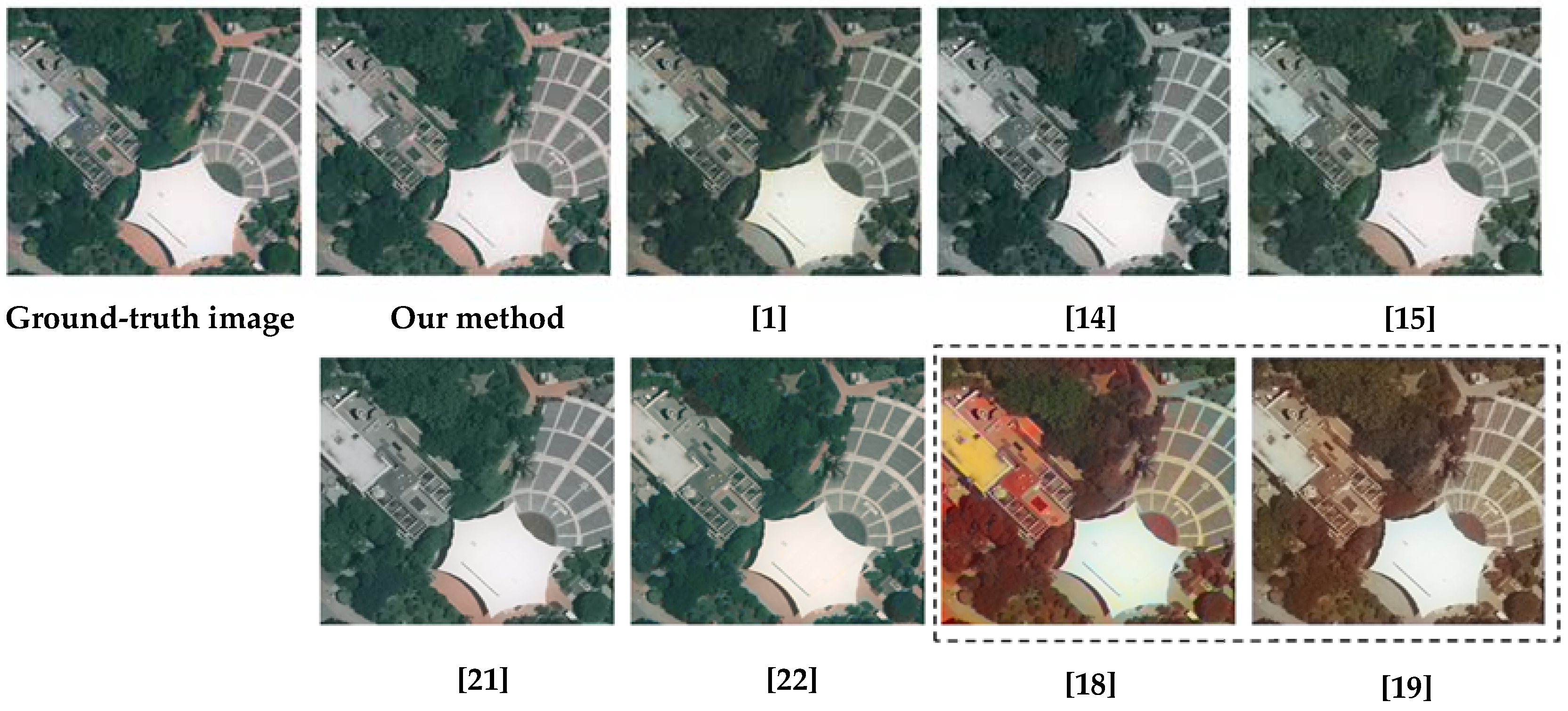
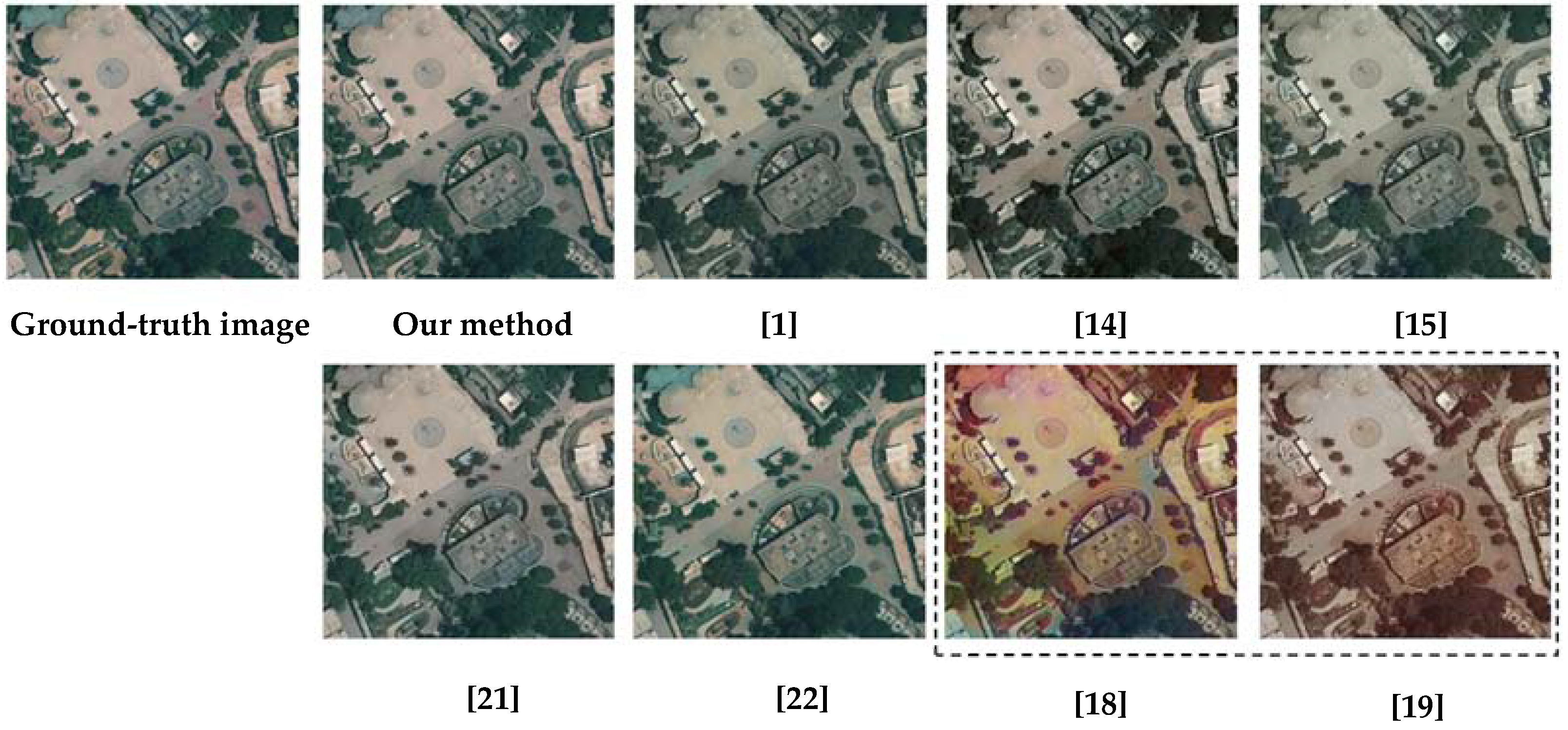
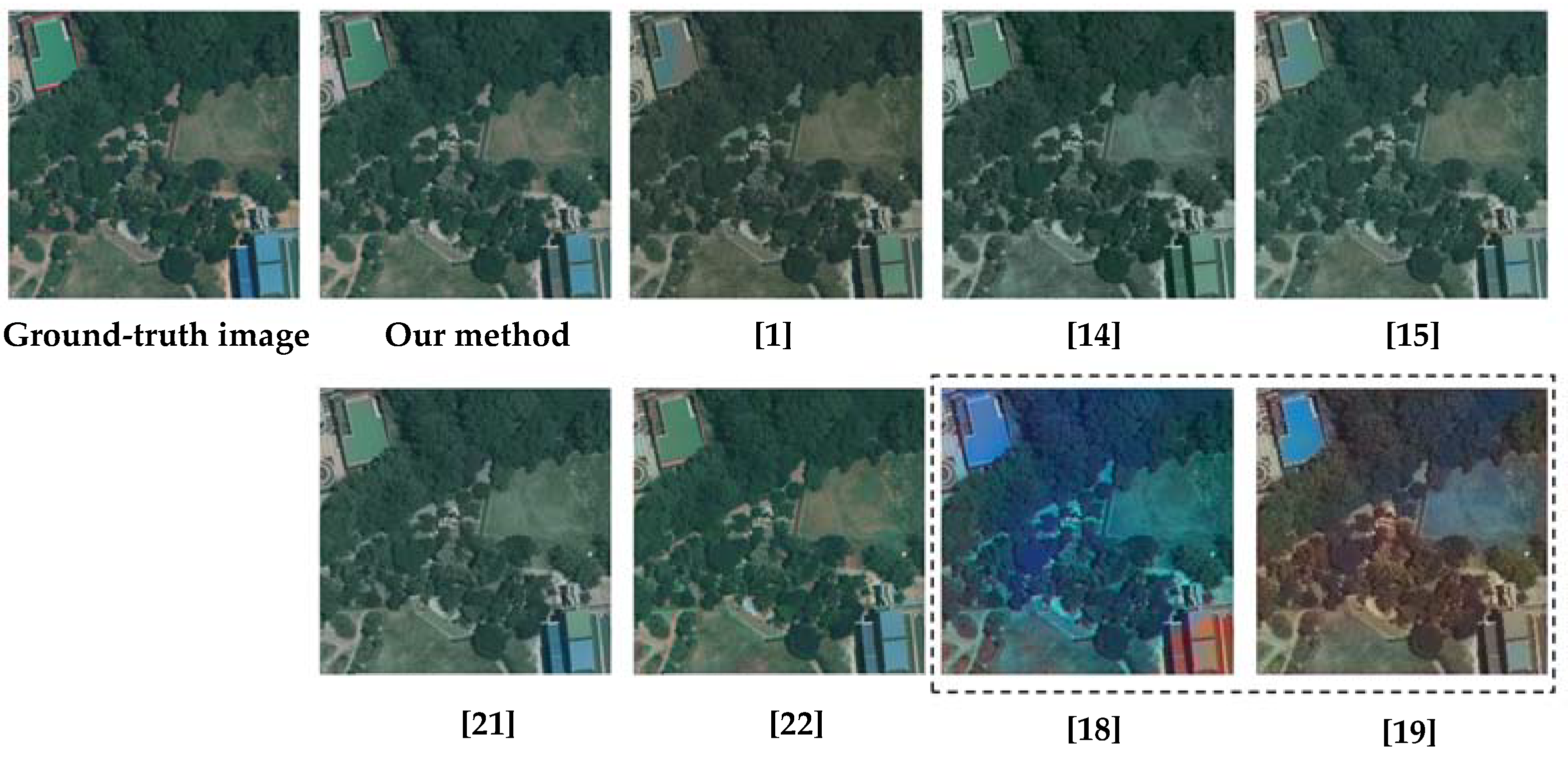
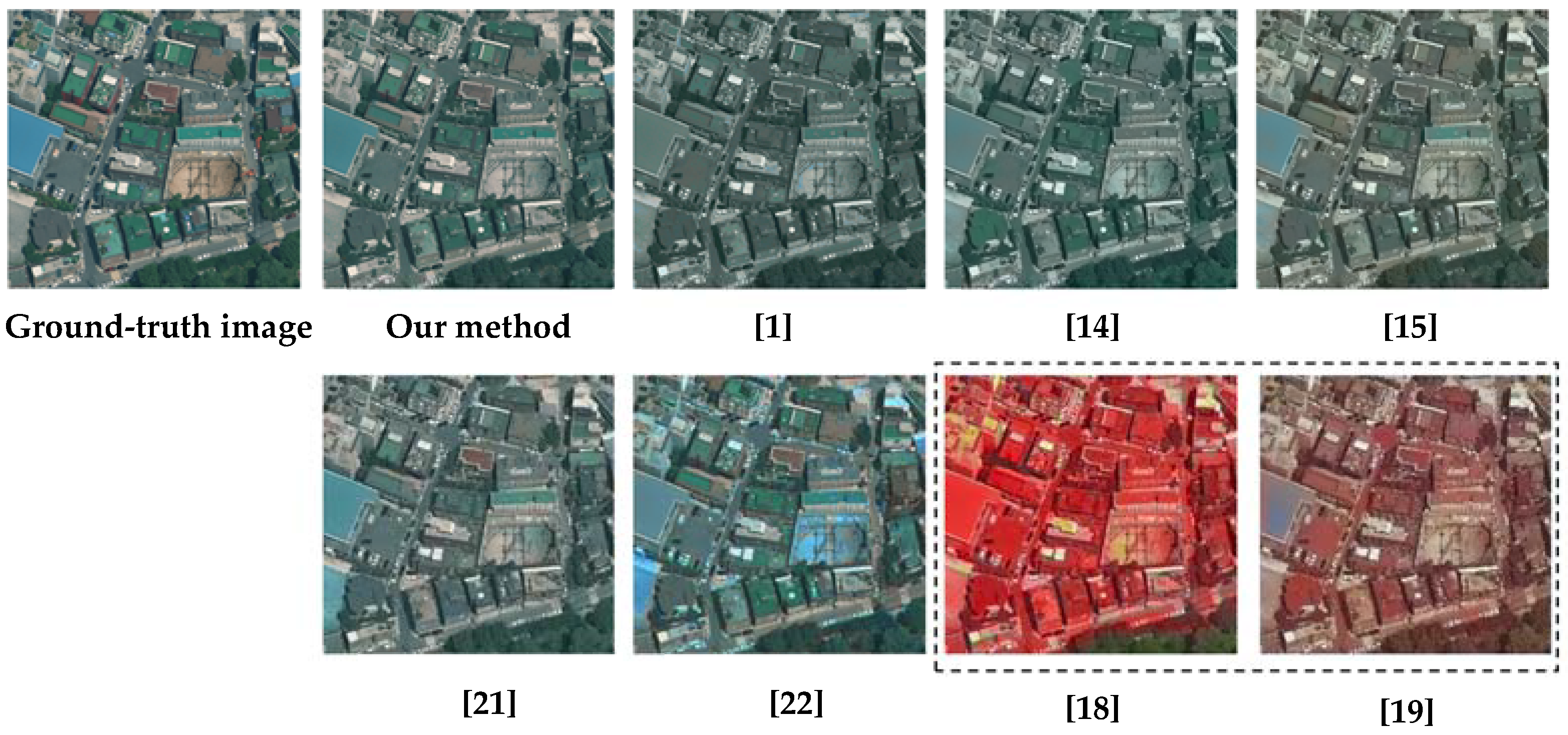
This section presents the colorization results of the proposed algorithm and compares these with the results of other state-of-the-art colorization algorithms. To ensure a fair comparison, colorization algorithms that use only a single-color image as the reference (exemplar-based method) and that are based on RF regression are compared, so that the methods of Welsh et al. [1], Bugeau et al. [14], Gupta et al. [15], Gupta et al. [21], and Deshpande et al. [22] are selected. When performing the colorization using these other methods, we used the same parameter settings suggested by their respective authors. In addition, two of the latest deep learning-based methods [18,19] are included for visual comparison, using the codes provided by the authors. The results of the various algorithms are compared by visual inspection (see Figure 6, Figure 7, Figure 8 and Figure 9) and quantitative evaluation with ground-truth images, which are the actual color images of the input grayscale images.
From the overall visual inspection, the proposed algorithms appear to show better results than do the five existing methods for most cases. The Welsh et al. method [1] is based on transferring color from one initial color image considered as an example. Color prediction is performed by minimizing the distance in the simple statistics of a luminance image. However, as the results show, only a few colors are dealt with, and the results include many artifacts due to the lack of any spatial coherency criteria. In the case of the Bugeau et al. method [14], image colorization is solved by computing the colors using different features and associated metrics. Then, the best colors are automatically selected via a variational framework. Overall, the results fail to select the best colors and have a desaturating effect, confirming the limitations of the variational framework. The Gupta et al. method [15] performs image colorization by automatically exploiting multiple image features. This method transfers color information by performing feature-matching between a reference color image and an input grayscale image—a process that is critical to the quality of the results. This achieves better colorization than the other exemplar-based methods but still only deals with a few colors, resulting in incorrect matches in challenging scenarios.
The other Gupta et al. method [21] is a learning-based method in which learning is performed in superpixel units to enforce higher color consistency. Superpixels are extracted, features are computed for each superpixel, and learning is performed based on an RF regression. The results of this method contain more color information than do the results of the other exemplar-based methods, but the approach still does not retrieve certain colors such as blue or red (Figure 7), and it sometimes predicts completely different colors (as in Figure 8 and Figure 9). The Deshpande et al. method [22] is also based on RF regression, which is performed within the LEArning to seaRCH (LEARCH) framework. Furthermore, histogram correction is performed on the colorization image to improve the visual appeal of the results. In the state-of-the-art-methods used for comparison, this method predicts sufficient color information. However, halo effects exist in the object boundaries, especially in Figure 7. Moreover, as shown in Figure 9, the more complex the structure, the more halo effects are added, leading to many artifacts.
In addition to exemplar-based and RF regression-based methods, deep learning-based methods [18,19] are used for comparison. These colorization algorithms use millions of images for training neural networks, which are based on ImageNet and convolutional neutral networks (CNN). Both results contain color information that is completely different from the ground-truth or reference color images, as shown in Figure 6, Figure 7, Figure 8 and Figure 9. For example, although the colors of the tree are somewhat predicted, the colors of the buildings or the roads are not predicted at all, which suggests that artifacts are more obvious when the structure is complex. In other words, it is impossible to colorize aerial images through a model that is trained with natural images.
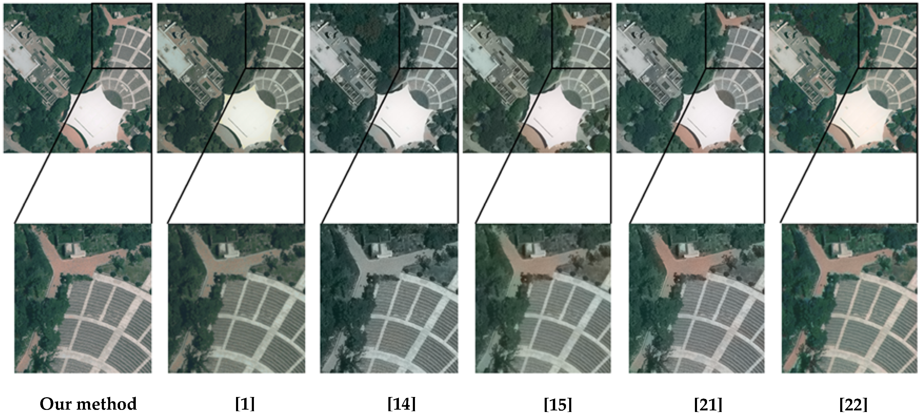
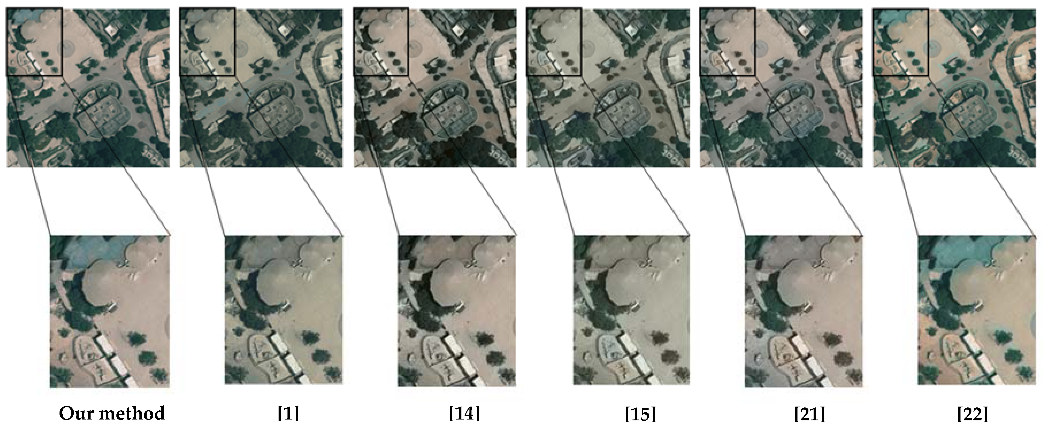
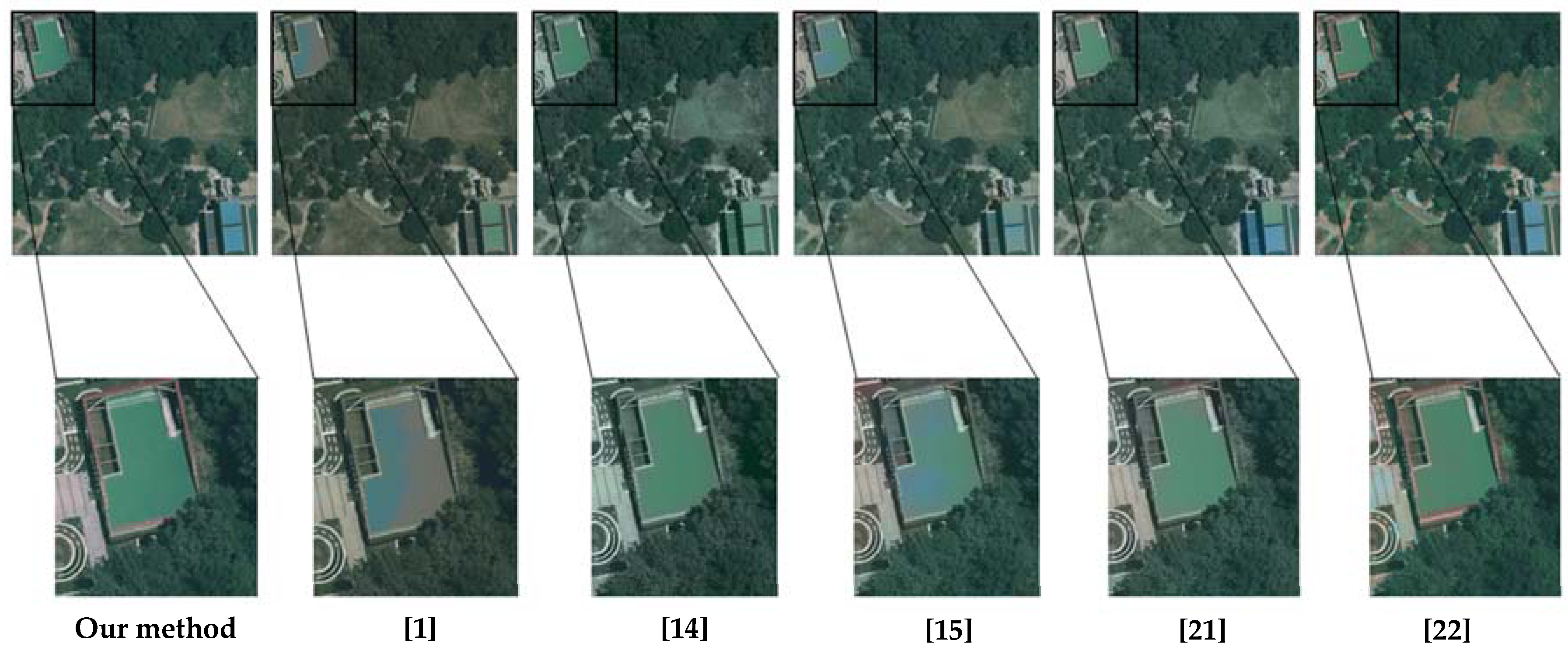
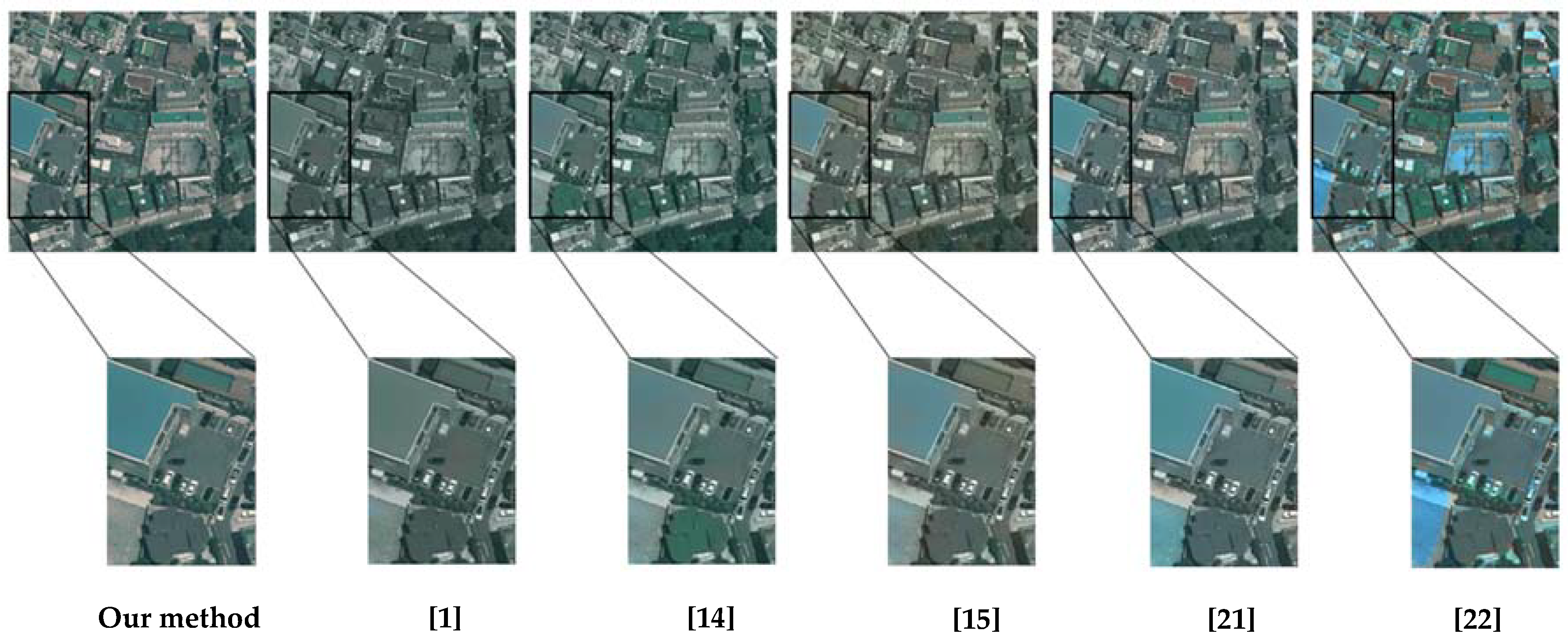
As can be seen in Figure 6, Figure 7, Figure 8 and Figure 9, our approach more accurately predicts colors than do the other methods, producing results with fewer artifacts. In Figure 6, the color determined by our method is much clearer, especially in the red portion of the ground that is correctly recovered without artifacts. Figure 7 is a site with many human-made objects, and our method demonstrates remarkably high performance in color prediction, while other methods completely fail to correctly predict colors or contain halo effects. Figure 8 also has many human-made objects that contain multiple colors in the area of vegetation, which makes it more difficult to predict the color values at this site. Except for our method and that of Deshpande et al. [22], the colors of human-made objects are not correctly predicted, which indicates that our method is robust for color prediction. Figure 9, the urban area, contains the most complex structure and the greatest variety of colors for prediction. Although the results of the proposed method also contain slightly turbid colors, our method produces significantly better results than do the other methods. In other words, our method retrieves more color values with fewer artifacts from the reference image; these details can be confirmed in Figure 10, Figure 11, Figure 12 and Figure 13.
Although visual inspection is a simple and direct way of appreciating the quality of the colorization results, it is highly subjective and cannot accurately evaluate the results of the various colorization methods. Therefore, for quantitative evaluation of the results, we employ the standard peak signal-to-noise ratio (PSNR) and normalized color difference (NCD). The PSNR, which is expressed in terms of the decibel (dB), is an estimate of the quality of the reconstructed (colorization) image compared with the ground-truth color image [54]. Given an m × n ground-truth color image u0 and a colorization result u, PSNR is defined as:
where MAXI is the maximum possible pixel value of the image (i.e., 255 with standard 8-bit samples), and ∑RGB() denotes summation over the red, green, and blue bands. The higher the PSNR value, the better the reconstruction process. Normalized color difference is used to measure the color quality degradation in color images [55]. For the NCD calculation, Lab space is used and is defined as:
where ΔL, Δa and Δb are the differences between the components of the ground-truth color image and the colorization result, and Lu0, au0, and bu0 are each component values of the ground-truth color image [56]. The lower the NCD value, the better the color quality.
The PSNRs and NCDs of the various algorithms are shown in Table 1 and Table 2. In the case of PSNR, the proposed method (Max: 35.0906, Min: 29.6542, Average (Avg): 32.8773) significantly outperforms those of Welsh et al. [1] (Max: 27.1564, Min: 23.5535, Avg: 25.9514), Bugeau et al. [14] (Max: 29.1172, Min: 26.2594, Avg: 27.5596), Gupta et al. [15] (Max: 30.6962, Min: 27.1006, Avg: 29.3068), Gupta et al. [21] (Max: 32.6280, Min: 28.0476, Avg: 30.6694), and Deshpande et al. [22] (Max: 31.5879, Min: 24.2211, Avg: 29.6766). The performance difference from the state-of-the-art methods ranges from 2.4626 to 7.9342 for the maximum PSNR, 1.6066–6.1007 for the minimum PSNR, and 2.1779–6.9259 for the average PSNR, which indicates high performance for all results, regardless of site. That is, it is possible to colorize images stably regardless of the object included in the image or the complexity of the included structure.
The NCD of the proposed method (Max: 0.0707, Min: 0.1244, Avg: 0.0941) also show better performance than do Welsh et al. [1] (Max: 0.1408, Min: 0.2304, Avg: 0.1819), Bugeau et al. [14] (Max: 0.1270, Min: 0.1722, Avg: 0.1561), Gupta et al. [15] (Max: 0.0963, Min: 0.1679, Avg: 0.1362), Gupta et al. [21] (Max: 0.0858, Min: 0.1422, Avg: 0.1148), and Deshpande et al. [22] (Max: 0.1042, Min: 0.1801, Avg: 0.1231), in which the range of the improved performance difference is 0.0151–0.0701 for the maximum NCD, 0.0178–0.1244 for the minimum NCD, and 0.0207–0.0878 in the average NCD. This means that the degradation in color quality is lowest when performing colorization through the proposed method. In other words, both visual and quantitative evaluations confirm the superiority of the method proposed herein.
3.2. Limitations
The results show that the proposed algorithm can realize better results than can the existing methods; however, there remain several limitations. Firstly, if there are errors in orthorectification or image registration, incorrect extraction can be performed during selection of the training pixels in the preprocessing step. Although RF regression is robust to training data, some color relationships can be established incorrectly. Secondly, our method retrieves more color values than do the other methods, but, if the structure is complex, it contains somewhat turbid colors. The histogram specification for the reference color image is performed by post-processing, but there are still limitations. Thirdly, in this study, aerial images three years apart are used. However, further verification is needed to determine the extent of the period in which the colorization can properly be performed. Finally, our method is established by directly correlating color relationships between the input grayscale image and the reference color image, making it dependent on the availability of reference color aerial imagery of the same input area with matching seasonal characteristics. Consequently, when suitable color aerial images are unavailable, colorization may fail.
4. Conclusions
This paper presents a colorization algorithm for aerial imagery. The proposed method uses a reference color image with similar seasonal features at the same location as an input grayscale image. The color space of the reference color image is converted to Lab, and unchanged regions are selected by applying change detection to the input grayscale image and the L component of the reference color image, which serves as meaningful training data. Moreover, color relationships are established in direct correspondence between the feature descriptors of the input grayscale image and the a and b components of the reference color image based on the RF regression. Finally, histogram specification is applied to the colorization image to improve the results and is compared with state-of-the-art methods. Experimental results for multiple sites show that our method achieves visually appealing colorizations with significantly improved quantitative performance. In other words, the proposed algorithm performs well and outperforms existing colorization approaches for aerial images.
Future work will include other complex descriptors or features in order to retrieve more color values for complex structures. In particular, we intend to find the combination of features that best describes the characteristics of the aerial images for colorization. We will also extend our application of the technique by applying satellite images obtained from various sensors other than aerial images. Furthermore, to overcome the limitations that may prevent colorization from being performed when reference color images are unavailable, a method of using reference color images that are obtained with different sensors or contain different seasons or resolutions will be sought out. Finally, we plan to colorize past grayscale aerial images using a time-series approach, possibly by incorporating monitoring frameworks.
Author Contributions
All authors contributed to the writing of the manuscript. D.K.S. carried out the experiments and analyzed the results; Y.H.K. designed the experiments and presented the direction of this study; Y.D.E. supervised this study; W.Y.P. provided scientific counsel.
Funding
This research was supported by the Basic Science Research Program through the NRF (National Research Foundation of Korea) funded by the Ministry of Education [No. 2016R1D1A1B03933562].
Conflicts of Interest
The authors declare no conflict of interest.
References
- Welsh, T.; Ashikhmi, M.; Mueller, K. Transferring Color to Grayscale Images. ACM Trans. Graph. 2002, 21, 277–280. [Google Scholar] [CrossRef]
- Bugeau, A.; Ta, V. Patch-Based Image Colorization. In Proceedings of the 21st International Conference on Pattern Recognition, Tsukuba, Japan, 11–15 November 2012; pp. 3058–3061. [Google Scholar]
- Lipowezky, U. Grayscale Aerial and Space Image Colorization Using Texture Classification. Pattern Recogn. Lett. 2005, 27, 275–286. [Google Scholar] [CrossRef]
- Yang, Y.; Wan, W.; Huang, S.; Lin, P.; Que, Y. A Novel Pan-Sharpening Framework Based on Matting Model and Multiscale Transform. Remote Sens. 2017, 9, 391. [Google Scholar] [CrossRef]
- Li, S.; Kang, X.; Fang, L.; Hu, J.; Yin, H. Pixel-Level Image Fusion: A Survey of the State of the Art. Inf Fusion. 2017, 33, 100–112. [Google Scholar] [CrossRef]
- Ghassemian, H. A Review of Remote Sensing Image Fusion Methods. Inf Fusion. 2016, 32, 75–89. [Google Scholar] [CrossRef]
- Horiuchi, T. Estimation of Color for Gray-Level Image by Probabilistic Relaxation. In Proceedings of the Object Recognition Supported by User Interaction for Service Robots, Quebec, Canada, 11–15 August 2002; pp. 867–870. [Google Scholar]
- Arbelot, B.; Vergne, R.; Hurtut, T.; Thollot, J. Automatic Texture Guided Color Transfer and Colorization. In Proceedings of the Joint Symposium on Computational Aesthetics and Sketch Based Interfaces and Modeling and Non-Photorealistic Animation and Rendering, Lisbon, Portugal, 7–9 May 2016; pp. 21–32. [Google Scholar]
- Li, B.; Lai, Y.K.; Rosin, P.L. Example-Based Image Colorization via Automatic Feature Selection and Fusion. Neurocomputing 2017, 266, 687–698. [Google Scholar] [CrossRef]
- Levin, A.; Lischinski, D.; Weiss, Y. Colorization Using Optimization. ACM Trans. Graph. 2004, 23, 689–694. [Google Scholar] [CrossRef]
- Huang, Y.C.; Tung, Y.S.; Chen, J.C.; Wang, S.W.; Wu, J.L. An Adaptive Edge Detection Based Colorization Algorithm and Its Applications. In Proceedings of the 13th ACM International Conference on Multimedia, Hilton, Singapore, 6–11 November 2005; pp. 351–354. [Google Scholar]
- Irony, R.; Cohen-Or, D.; Lischinski, D. Colorization by Example. In Proceedings of the Sixteen Eurographics Conference on Rendering Techniques, Konstanz, Germany, 29 June–1 July 2005; pp. 201–210. [Google Scholar]
- Yatziv, L.; Sapiro, G. Fast Image and Video Colorization Using Chrominance Blending. IEEE Trans. Image Process. 2006, 15, 1120–1129. [Google Scholar] [CrossRef] [PubMed]
- Bugeau, A.; Ta, V.T.; Papadakis, N. Variational Exemplar-Based Image Colorization. IEEE Trans. Image Process. 2014, 23, 298–307. [Google Scholar] [CrossRef] [PubMed] [Green Version]
- Gupta, R.L.; Chia, A.Y.S.; Rajan, D.; Ng, E.S.; Zhiyoung, H. Image Colorization Using Similar Images. In Proceedings of the 20th ACM International Conference on Multimedia, Nara, Japan, 29 October–2 November 2012; pp. 369–378. [Google Scholar]
- Charpiat, G.; Hofmann, M.; Scholkopf, B. Automatic Image Colorization via Multimodal Predictions. In Proceedings of the 10th European Conference on Computer Vision, Marseille, France, 12–18 October 2008; pp. 126–139. [Google Scholar]
- Cheng, Z.; Yang, Q.; Sheng, B. Deep Colorization. In Proceedings of the IEEE International Conference on Computer Vision, Santiago, Chile, 7–13 December 2015; pp. 415–423. [Google Scholar]
- Zhang, R.; Isola, P.; Efros, A.A. Colorful Image Colorization. In Proceedings of the Computer Vision—ECCV 2016—14th European Conference, Amsterdam, The Netherlands, 11–14 October 2016; pp. 649–666. [Google Scholar]
- Larrson, G.; Maire, M.; Shakhnarovich, G. Learning Representations for Automatic Colorization. In Proceedings of the Computer Vision—ECCV 2016—14th European Conference, Amsterdam, The Netherlands, 11–14 October 2016; pp. 577–593. [Google Scholar]
- Brieman, L. Random Forests. Mach. Learn. 2001, 45, 5–32. [Google Scholar] [CrossRef] [Green Version]
- Gupta, R.K.; Chia, A.Y.; Rajan, D.; Zhiyong, H. A Learning-based Approach for Automatic Image and Video Colorization. In Proceedings of the Computer Graphics International, Bournemouth, UK, 12–15 June 2012; pp. 1–10. [Google Scholar]
- Deshpande, A.; Rock, J.; Forsyth, D. Learning Large-Scale Automatic Image Colorization. In Proceedings of the 2015 IEEE International Conference on Computer Vision, Santiago, Chile, 7–13 December 2015; pp. 567–575. [Google Scholar]
- Mohn, H.; Caebelein, M.; Hansch, R.; Hellwich, O. Towards Image Colorization with Random Forests. In Proceedings of the 13th International Joint Conference on Computer Vision, Funchal, Madeira, Portugal, 27–29 January 2018; pp. 270–278. [Google Scholar]
- Culter, D.R.; Edwards, T.C.; Beard, K.H.; Culter, A.; Hess, K.T.; Gibson, J.C. Random Forests for Classification in Ecological Society of America. Ecology 2007, 88, 2783–2792. [Google Scholar] [CrossRef]
- Yang, Y.; Cao, C.; Pan, X.; Li, X.; Zhu, X. Downscaling Land Surface Temperature in an Arid Area by Using Multiple Remote Sensing Indices with Random Forest Regression. Remote Sens. 2017, 9, 789. [Google Scholar] [CrossRef]
- Shataee, S.; Kalbi, S.; Fallah, A.; Pelz, D. Forest Attribute Imputation Using Machine Learning Methods and ASTER Data: Comparison of K-NN, SVR, Random Forest Regression Algorithms. Int. J. Remote Sens. 2012, 33, 6254–6280. [Google Scholar] [CrossRef]
- Peters, J.; Baets, B.D.; Verhoest, N.E.C.; Samson, R.; Degroeve, S.; Becker, P.D.; Huybrechts, W. Random Forests as a Tool for Ecohydrological Distribution Modeling. Ecol. Model. 2007, 207, 304–318. [Google Scholar] [CrossRef]
- Rodriguez-Galiano, V.; Sanchez-Castillo, M.; Olmo-Chica, M.; Chica-Rivas, M. Machine Learning Predictive Models for Mineral Prospectivity: An Evaluation of Neural Networks, Random Forest, Regression Trees and Support Vector Machines. Ore Geol. Rev. 2015, 71, 804–818. [Google Scholar] [CrossRef]
- Prasad, A.M.; Iverson, L.R.; Liaw, A. Newer Classification and Regression Tree Techniques: Bagging and Random Forests for Ecological Prediction. Ecosystems 2006, 9, 181–199. [Google Scholar] [CrossRef]
- Hutengs, C.; Vohland, M. Downscaling Land Surface Temperature at Regional Scales with Random Forest Regression. Remote Sens. Environ. 2016, 178, 127–141. [Google Scholar] [CrossRef]
- Changas, C.S.; Junior, W.C.; Behring, S.B.; Filho, B.G. Spatial Prediction of Soil Surface Texture in a Semiarid Region Using Random Forest and Multiple Linear Regressions. Catena 2016, 139, 232–240. [Google Scholar] [CrossRef]
- Scornet, E. Tuning Parameters in Random Forests. In Proceedings of the ESAIM: Proceedings and Surveys, Grenoble, France, 29–31 August 2017; pp. 144–162. [Google Scholar]
- Lawrence, R.L.; Wood, S.D.; Sheley, R.L. Mapping Invasive Plants Using Hyperspectral Imagery and Breiman Cutler Classification (RandomForest). Remote Sens. Environ. 2016, 100, 356–362. [Google Scholar] [CrossRef]
- Belgiu, M.; Dragut, L. Random Forest in Remote Sensing: A Review of Applications and Future Directions. ISPRS J. Photogramm. Remote Sens. 2015, 114, 24–31. [Google Scholar] [CrossRef]
- Seo, D.K.; Kim, Y.H.; Eo, Y.D.; Park, W.Y.; Park, H.C. Generation of Radiometric, Phenological Normalized Image Based on Random Forest Regression for Change Detection. Remote Sens. 2017, 9, 1163. [Google Scholar] [CrossRef]
- Sug, H. Applying Randomness Effectively Based on Random Forest for Classification Task of Datasets of Insufficient Information. J. Appl. Math. 2012, 2012, 1–13. [Google Scholar] [CrossRef]
- Palmer, D.S.; O’Boyle, N.M.; Glen, R.C.; Mitchell, J.B.O. Random Forest Models to Predict Aqueous Solubility. J. Chem. Inf. Model. 2007, 47, 150–158. [Google Scholar] [CrossRef] [PubMed]
- Dye, M.; Mutanga, O.; Ismail, R. Combining Spectral and Textural Remote Sensing Variables Using Random Forests: Predicting the Age of Pinus Forests in KwaZulu-Natal, South Africa. J. Spat Sci. 2012, 57, 193–211. [Google Scholar] [CrossRef]
- Quintana, D.; Saez, Y.; Isasi, P. Random Forest Prediction of IPO Underpricing. Appl. Sci. 2017, 7, 636. [Google Scholar] [CrossRef]
- Hussain, M.; Chen, D.; Cheng, A.; Wei, H.; Stanley, D. Change Detection from Remotely Sensed Images: From Pixel-Based to Object-Based Approaches. ISPRS J. Photogramm. Remote Sens. 2013, 80, 91–106. [Google Scholar] [CrossRef]
- Xiao, P.; Zhang, X.; Wang, D.; Yuan, M.; Feng, X.; Kelly, M. Change Detection of Built-up Land: A Framework of Combining Pixel-Based Detection and Object-Based Recognition. ISPRS J. Photogramm. Remote Sens. 2016, 119, 402–414. [Google Scholar] [CrossRef]
- Wang, J.; Qin, Q.; Gao, Z.; Zhao, J.; Ye, X. A New Approach to Urban Road Extraction Using High-Resolution Aerial Image. Int. J. Geo-Inf. 2016, 5, 114. [Google Scholar] [CrossRef]
- Crommelinck, S.; Bennett, R.; Gerke, M.; Koeva, M.N.; Yang, M.Y.; Vosselman, G. SLIC Superpixels for Object Delineation from UAV Data. In Proceedings of the International Conference on Unmanned Aerial Vehicles in Geomatics, Bonn, Germany, 4–7 September 2017; pp. 9–16. [Google Scholar]
- Mei, T.; An, L.; Li, Q. Supervised Segmentation of Remote Sensing Image Using Reference Descriptor. IEEE Geosci. Remote Sens. Lett. 2015, 12, 938–942. [Google Scholar] [CrossRef]
- Csillik, O. Fast Segmentation and Classification of Very High Resolution Remote Sensing Data Using SLIC Superpixels. Remote Sens. 2017, 9, 243. [Google Scholar] [CrossRef]
- Achanta, R.; Shaji, A.; Smith, K.; Luchi, A.; Fua, P.; Susstrunk, S. SLIC Superpixels Compared to State-of-the-Art Superpixels Methods. IEEE Trans. Pattern Anal. Mach. Intell. 2012, 34, 2274–2281. [Google Scholar] [CrossRef] [PubMed]
- Zainal, Z.; Ramli, R.; Mustafa, M.M. Grey-Level Cooccurence Matrix Performance Evaluation for Heading Angle Estimation of Movable Vision System in Static Environment. J. Sens. 2013, 2013, 1–15. [Google Scholar] [CrossRef]
- Zhang, X.; Cui, J.; Wang, W.; Lin, C. A Study for Texture Feature Extraction of High-Resolution Satellite Images Based on a Direction Measure and Gray Level Co-Occurrence Matrix Fusion Algorithm. Sensors 2017, 17, 1474. [Google Scholar] [CrossRef] [PubMed]
- Huang, X.; Liu, X.; Zhang, L. A Multichannel Gray Level Co-Occurrence Matrix for Multi/Hyperspectral Image Texture Representation. Remote Sens. 2014, 6, 8424–8445. [Google Scholar] [CrossRef] [Green Version]
- Jia, B.; Wang, W.; Yoon, S.C.; Zhuang, H.; Li, Y.F. Using a Combination of Spectral and Texture Data to Measure Water-Holding Capacity in Fresh Chicken Breas Fillets. Appl. Sci. 2018, 8, 343. [Google Scholar] [CrossRef]
- Zheng, S.; Zheng, J.; Shi, M.; Li, X. Classification of Cultivated Chinese Medicinal Plants Based on Fractal Theory and Gray Level Co-Occurrence Matrix Textures. J. Remote Sens. 2014, 18, 868–886. [Google Scholar] [CrossRef]
- Sun, C.C.; Ruan, S.J.; Shie, M.C.; Pai, T.W. Dynamic Contrast Enhancement Based on Histogram Specification. IEEE Trans. Consum. Electron. 2005, 51, 1300–1305. [Google Scholar] [CrossRef]
- Xie, L.; Wang, G.; Zhang, X.; Xiao, B.; Zhou, B.; Zhang, F. Remote Sensing Image Enhancement Based on Wavelet Analysis and Histogram Specification. In Proceedings of the 2014 IEEE 3rd International Conference on Cloud Computing and Intelligence Systems, Shenzhen, China, 27–29 November 2014; pp. 55–59. [Google Scholar]
- Al-Najjar, Y.; Chen, S.D. Comparison of Image Quality Assessment: PSNR, HVS, SSIM, UIQI. Int. J. Sci. Eng. Res. 2012, 3, 1–5. [Google Scholar]
- Senthilkumaran, N.; Saromary, J. Detailed Performance Evaluation of Bilateral Filters for De-noising Chromosome Image. Int. J. Inf. Technol. 2017, 3, 64–70. [Google Scholar]
- Szczepanski, M.; Smolka, B.; Plataniots, K.N.; Ventesanopoulos, A.N. On the Distance Function Approach to Color Image Enhancement. Discret.Appl. Math. 2004, 139, 283–305. [Google Scholar] [CrossRef]
Figure 1.
Experimental area of site 1: (a) input grayscale image acquired on 10 June 2013, (b) reference color image acquired on 2 June 2016.
Figure 1.
Experimental area of site 1: (a) input grayscale image acquired on 10 June 2013, (b) reference color image acquired on 2 June 2016.

Figure 2.
Experimental area of site 2: (a) input grayscale image acquired on 10 June 2013, (b) reference color image acquired on 2 June 2016.
Figure 2.
Experimental area of site 2: (a) input grayscale image acquired on 10 June 2013, (b) reference color image acquired on 2 June 2016.

Figure 3.
Experimental area of site 3: (a) input grayscale image acquired on 10 June 2013, (b) reference color image acquired on 2 June 2016.
Figure 3.
Experimental area of site 3: (a) input grayscale image acquired on 10 June 2013, (b) reference color image acquired on 2 June 2016.

Figure 4.
Experimental area of site 4: (a) input grayscale image acquired on 10 June 2013, (b) reference color image acquired on 2 June 2016.
Figure 4.
Experimental area of site 4: (a) input grayscale image acquired on 10 June 2013, (b) reference color image acquired on 2 June 2016.

Figure 5.
The flowchart of the proposed method. RGB: Red-Green-Blue color space, Lab: CIE L*a*b color space, L component: grayscale axis, a and b components: two-color axes, RF: random forest.
Figure 5.
The flowchart of the proposed method. RGB: Red-Green-Blue color space, Lab: CIE L*a*b color space, L component: grayscale axis, a and b components: two-color axes, RF: random forest.

Figure 6.
Comparison with existing state-of-the-art colorization methods at site 1.

Figure 7.
Comparison with existing state-of-the-art colorization methods at site 2.

Figure 8.
Comparison with existing state-of-the-art colorization methods at site 3.

Figure 9.
Comparison with existing state-of-the-art colorization methods at site 4.

Figure 10.
Enlargement of site 1: our method retrieves color values well in this region, compared with other methods.
Figure 10.
Enlargement of site 1: our method retrieves color values well in this region, compared with other methods.

Figure 11.
Enlargement of site 2: our method retrieves color values well in this region, compared with other methods.
Figure 11.
Enlargement of site 2: our method retrieves color values well in this region, compared with other methods.

Figure 12.
Enlargement of site 3: our method retrieves color values well in this region, compared with other methods.
Figure 12.
Enlargement of site 3: our method retrieves color values well in this region, compared with other methods.

Figure 13.
Enlargement of site 4: our method retrieves color values well in this region, compared with other methods.
Figure 13.
Enlargement of site 4: our method retrieves color values well in this region, compared with other methods.


Table 1.
Quantitative evaluation of algorithm performance using standard peak signal-to-noise ratio (PSNR). dB: decibel.
Table 1.
Quantitative evaluation of algorithm performance using standard peak signal-to-noise ratio (PSNR). dB: decibel.
| PSNR (dB) | ||||||
|---|---|---|---|---|---|---|
| Method | Our Method | [1] | [14] | [15] | [21] | [22] |
| Site 1 | 35.0906 | 26.9364 | 29.1172 | 30.6962 | 32.628 | 31.5879 |
| Site 2 | 34.8936 | 27.1564 | 26.2594 | 29.9741 | 31.6331 | 31.8681 |
| Site 3 | 31.8709 | 26.1595 | 28.0316 | 29.4565 | 30.369 | 31.0295 |
| Site 4 | 29.6542 | 23.5535 | 26.8302 | 27.1006 | 28.0476 | 24.2211 |
Table 2.
Quantitative evaluation of algorithm performance using normalized color difference (NCD).
| NCD | ||||||
|---|---|---|---|---|---|---|
| Method | Our Method | [1] | [14] | [15] | [21] | [22] |
| Site 1 | 0.0707 | 0.1472 | 0.127 | 0.0963 | 0.0858 | 0.1042 |
| Site 2 | 0.0716 | 0.1408 | 0.1573 | 0.1334 | 0.0929 | 0.1069 |
| Site 3 | 0.1098 | 0.2094 | 0.1722 | 0.1472 | 0.1386 | 0.1373 |
| Site 4 | 0.1244 | 0.2304 | 0.1677 | 0.1679 | 0.1422 | 0.1801 |
© 2018 by the authors. Licensee MDPI, Basel, Switzerland. This article is an open access article distributed under the terms and conditions of the Creative Commons Attribution (CC BY) license (http://creativecommons.org/licenses/by/4.0/).
Share and Cite
MDPI and ACS Style
Seo, D.K.; Kim, Y.H.; Eo, Y.D.; Park, W.Y. Learning-Based Colorization of Grayscale Aerial Images Using Random Forest Regression. Appl. Sci. 2018, 8, 1269. https://doi.org/10.3390/app8081269
AMA Style
Seo DK, Kim YH, Eo YD, Park WY. Learning-Based Colorization of Grayscale Aerial Images Using Random Forest Regression. Applied Sciences. 2018; 8(8):1269. https://doi.org/10.3390/app8081269
Chicago/Turabian StyleSeo, Dae Kyo, Yong Hyun Kim, Yang Dam Eo, and Wan Yong Park. 2018. "Learning-Based Colorization of Grayscale Aerial Images Using Random Forest Regression" Applied Sciences 8, no. 8: 1269. https://doi.org/10.3390/app8081269
Note that from the first issue of 2016, this journal uses article numbers instead of page numbers. See further details here.