Acceleration Harmonics Identification for an Electro-Hydraulic Servo Shaking Table Based on a Nonlinear Adaptive Algorithm

Abstract

Since the electro-hydraulic servo shaking table came into existence, many nonlinear elements, such as, dead zone, friction and backlash, as well as its acceleration response has higher harmonics which result in acceleration harmonic distortion, when the electro-hydraulic system is excited by sinusoidal signal. For suppressing the harmonic distortion and precisely identify harmonics, a combination of the adaptive linear neural network and least mean M-estimate (ADALINE-LMM), is proposed to identify the amplitude and phase of each harmonic component. Specifically, the Hampel’s three-part M-estimator is applied to provide thresholds for detecting and suppressing the impulse noise. Harmonic generators are used by this harmonic identification scheme to create input vectors and the value of the identified acceleration signal is subtracted from the true value of the system acceleration response to construct the criterion function. The weight vector of the ADALINE is updated iteratively by the LMM algorithm, and the amplitude and phase of each harmonic, even the results of harmonic components, can be computed directly online. The simulation and experiment are performed to validate the performance of the proposed algorithm. According to the experiment result, the above method of harmonic identification possesses great real-time performance and it has not only good convergence performance but also high identification precision.

1. Introduction

As a great significant testing equipment for engineering research in industry, the electro-hydraulic servo shaking table has some advantages, such as quicker response speed, higher control precision, higher force-to weight ratio, etc. These make it suited to be applied in aerospace, automotive, machine, metallurgy and many other fields of heavy-industries [1]. Yet the electro-hydraulic servo shaking table also has plenty of disadvantages, namely, the dead zone of the servo valve, backlash connections, friction between the piston and the hydraulic cylinder, and the hydraulic oil pipeline geometry [2,3]. The dead zone is time-varying and asymmetrical, which is caused by the overlap of the slide valve and has a bad influence on static deviation of the system [4]. Friction and the hydraulic oil pipeline geometry will influence dynamic and fast-tracing performance of the electro-hydraulic shaking table system [4]. These existing nonlinear elements are inherent characteristics of the hydraulic system which cannot be avoided physically. As the impact of these nonlinearities existing in the servo system, the acceleration response of system generates high-order harmonics when the shaking table is excited by sinusoidal signal, which not only seriously leads to distortion of the acceleration response signal, but also lowers the dynamic tracing performance. Definitely, under this condition, the control precision of the system will decrease. Sometimes, these aforementioned nonlinearities existing in the system may even make the electro-hydraulic servo shaking table unstable.

Although the harmonic identification is mostly applied in the field of the power system, it is still meaningful for us to apply it to the electro-hydraulic servo shaking table system. In the power system field, in order to guarantee the power quality, researchers who devote themselves into this field propose various techniques such as Fast Fourier Transformation (FFT), Kalman Filter (KF), Least Mean Square (LMS), Recursive Least Squares (RLS) and many other algorithms to identify the high order harmonics of the current signal [5,6]. However, the FFT estimation algorithm need to acquire the past current data firstly, then analyze it. The computation task of using FFT to identify harmonics is burden and it inevitably gets delayed for about two periods. Furthermore, the real-time performance of this algorithm is not good. The precision of the estimated parameter may decrease due to frequency spectrum leakage and picket-fence effects. Kalman Filter is also one of the most useful algorithms for harmonic identification, but its dynamic tracing performance will be seriously reduced when the tested signal is time-varying. Besides, Least Mean Square, as well as Recursive Least Squares, is also used in harmonic identification. But they are not that effective when used to estimate harmonics online. During the real-time detection, since their estimation precision and real-time performance are unqualified, they are not extensively used.

The artificial neural network (ANN) is a network that is combined with several nerve cells. It is an important way to imitate human intelligence from microcosmic structure and function. It certainly reflects some basic characters of human brain’s function. After several intensive studies, scientists proposed lots of ways to identify high order harmonics. Yao et al. [3] developed a new adaptive linear neural network using normalized least-mean-square adaptive algorithm to adjust the value of weight for harmonic identification in an electro-hydraulic servo shaking table system. Cao et al. [7] proposed a new method based on Radial basis function (RBF) neural network to detect each order harmonic’s amplitude and phase of a distorted harmonic signal. Ketabi et al. [8] introduced a multilayer feedforward neural network to analyze harmonic overvoltage during power system restoration. The effect and precision performance of this scheme had been proved to be satisfied by experimental results. Based on Hopfield neural network, Zou et al. [9] proposed a new approach using for harmonic detection, and the convergence and real-time performance was proved to be satisfied. A parallel neural networks-based method was adopted by Nascimento to identify harmonics in single phase systems [10]. Subsequently, the adaptive linear neural network (Adaline) is extensively applied for harmonic parameters estimation, and the Least mean square (LMS) algorithm is used to adjust the weight of the Adaline. But if the tested signal is distorted by impulse noise, the performance of linear adaptive filter with LMS-based algorithms will significantly degrade.

For impulse noise suppression, a new adaptive filtering algorithm using M-estimate was carried out by Zou to solve this problem [11]. M-estimate is a piecewise estimator which can detect impulse noise and ignore the large signal error when the measured signal is contaminated by the impulse signal. For active impulse-like noise control, Wu [12] proposed a new M-estimator based algorithm called fair algorithm and its effectiveness and convergence performance were validated by the simulation results. In 2000, Zou et al. [13] proposed two new gradient-based adaptive algorithms named the transform domain least mean M-estimate (TLMM) and the least Mean M-estimate (LMM) algorithms which possess better convergence and anti-impulse noise performance than RLS and LMS according to the simulation result. Based on the robust statistics theory, Sun et al. [14] proposed the filtered-x least mean M-estimate (FxLMM) algorithm to get a better noise control effect on active noise control (ANC). It was proved to be a very promising way for ANC with numerous simulation results.

The most obvious distinction between harmonic identification for electro-hydraulic servo shaking table system and for power system is that the former requires better real-time and precision performance [15,16]. Furthermore, harmonic distortion existing in an electro-hydraulic shaking table is dynamic and has notable nonlinear characteristics. However, the aforementioned harmonic identification methods can only be used to identify harmonics offline and their convergence and dynamic tracing performance have a significant decline when the system response is contaminated by the impulse noise. Unlike other abovementioned algorithms, the LMM algorithm, a LMS-like algorithm, uses a more robust “M-estimator” to replace LMS for the purpose of harmonic identification. Instead of minimizing the variance of the error signal directly, it chooses to minimize the M-estimate of the error signal and can be effectively used to detect and suppress the impulse noise, which is verified by simulation results. Furthermore, good precision identification results, both the amplitude and the phase of harmonics, are shown by using the Hampel’s three-part M-estimator. In this article, The LMM algorithm is utilized to adjust the weight of the Adaline for harmonic identification, and, subsequently, its numerous merits are verified through simulation and experimentation.

2. System Description

Figure 1 shows the electro-hydraulic servo shaking table of the University of Bristol. The table which is used to perform experiments in this paper is a platform made of cast aluminum weighing 3.8 tons. The maximum payload and the supply pressure of this table are 15 tons and 20.5 MPa separately. Other parameters are shown in

Table 1. The detail parameters of the shaking table.

Category	Parameter Value
Axes	6
Size	3 × 3 m
Frequency range	0–100 Hz
Vertical actuators	4 at 70 kN
Vertical acceleration (no payload)	5.6 g
Longitudinal and lateral actuators	4 at 70 kN
Horizontal acceleration (no payload)	3.7 g

. At the center of the table, an accelerometer is installed on the platform. Each actuator of this table contains an accelerometer at the end of the piston and a linear variable differential transformer (LVDT) fixed to the inside of the cylinder. Besides, the load applied by each actuator is measured by some load cells. The shaking table adopts a typical PID control system as its control system. The feedback signal of PID is usually a composite signal which includes the displacement signals, acceleration signals and load signals.

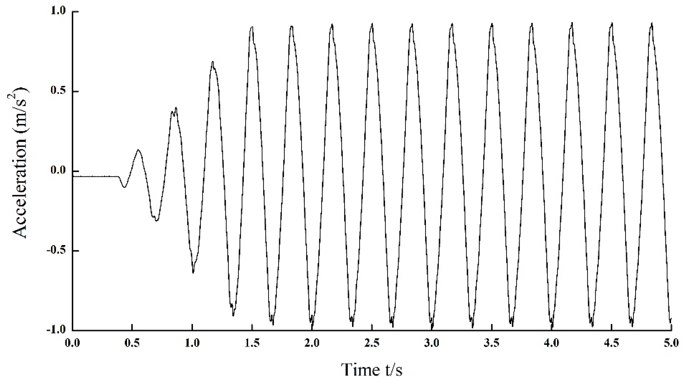
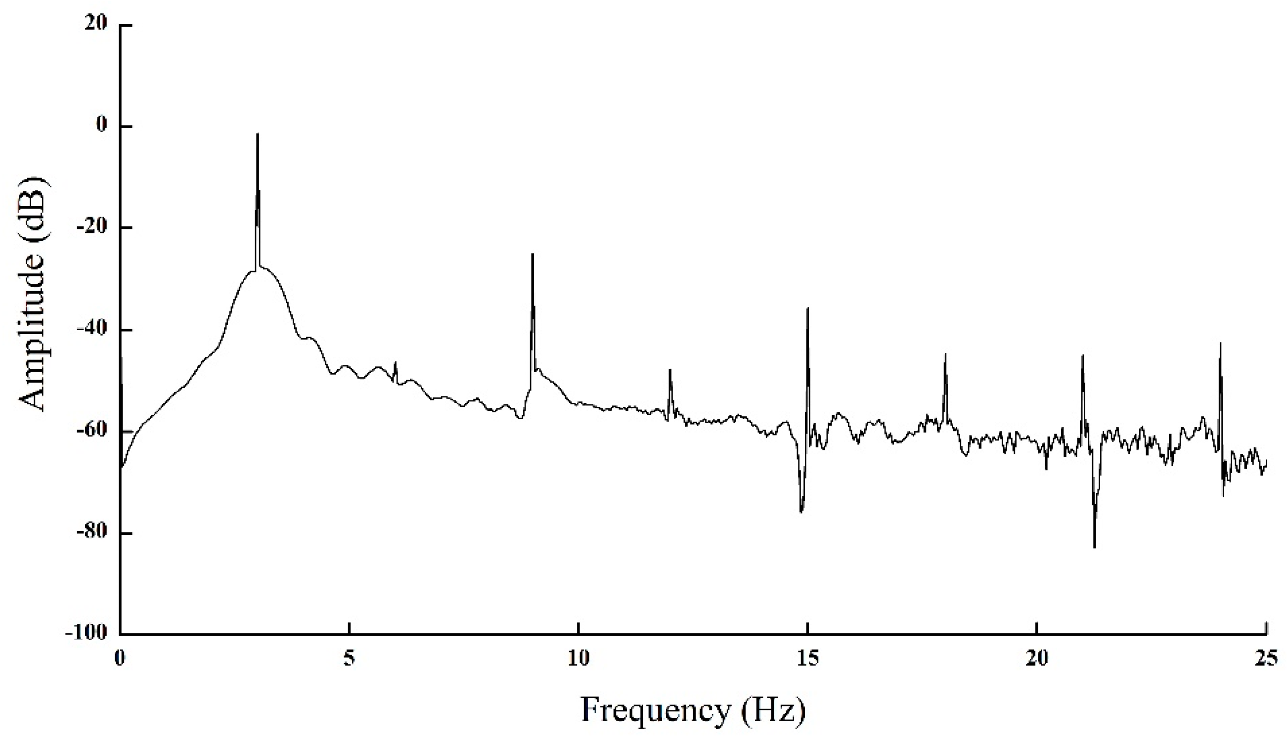
When the hydraulic servo shaking table without load is excited by a sinusoidal signal, $\sin (2\pi \times 3t)$ m/s², its corresponding sinusoidal acceleration response is shown in Figure 2. In time domain, it is clear that the acceleration response is not a standard sine wave but a distorted one. There are other seven harmonics (from the second to the eighth) except the fundamental frequency signal in the sinusoidal acceleration response shown in Figure 2 and Figure 3. Besides, in order to demonstrate the impact of the nonlinear hydraulic system, the total harmonic distortion (THD) is introduced. The value of THD can be calculated by using Equation (1), and its analysis result is shown in

Table 2. Total harmonic distortion (THD) analysis results.

THD	Harmonic Amplitude (m/s2)
7.06%	Fundamental	Second	Third	Fourth	Fifth	Sixth	Seventh	eighth
	0.859	0.005	0.057	0.004	0.016	0.006	0.006	0.008

. From Table 2, it can be seen that the amplitude of the fundamental response is less than the excitation signal. Besides, the third harmonic is the largest harmonic among other seven harmonics, i.e., it plays a most prominent part in THD. The amplitude of the sixth harmonic is the same as that of the Seventh, at 0.006, but both are less than the eighth harmonic. The fifth harmonic is in the least domination, at 0.016. The value of the THD is 7.06%.

$$THD=\frac{\sqrt{A_2{}^2+A_3{}^2+\cdots +A_n{}^2}}{A_1}\times 100\%$$

(1)

where $A_1,A_2,\cdots ,A_n$ are the amplitude of each harmonic separately.

3. Harmonic Identification Scheme Based on Adaline-LMM Algorithm

When the servo system is excited by a sinusoidal signal, the system response can be regarded as a composite signal which is composed of the fundamental response and high order harmonics. The general model of the composite signal can be defined as:

$$a(k)={\displaystyle \sum _{i=1}^N{A}_i\sin (i\omega k+{\phi }_i)}$$

(2)

where $A_i$, ${\phi }_i$ are the amplitude and phase of the ith harmonic, respectively. $\omega$ is the fundamental frequency. N is the highest order of the acceleration harmonic. k represents iterations. For the purpose of obtaining the input vector of the network, Equation (2) can be written as:

$$a(k)={\displaystyle \sum _{i=1}^N{A}_i\sin (i\omega k)\cos ({\phi }_i)+A_i\cos (i\omega k)\sin ({\phi }_i)}$$

(3)

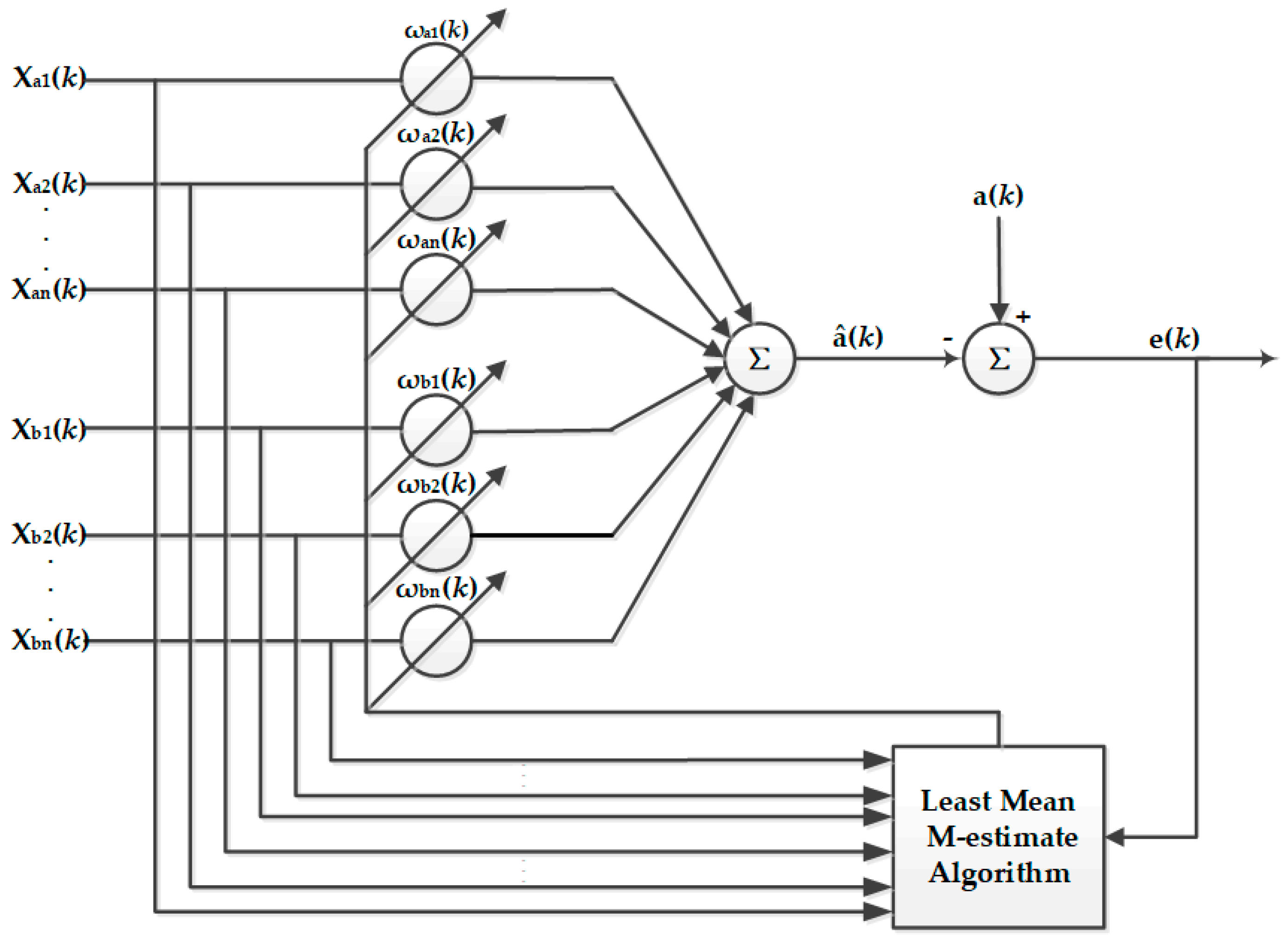
The scheme of the proposed harmonic identification method is illustrated in Figure 4. For identifying the fundamental waveform and high order harmonics, the Adaline is introduced. It is a single layer linear neural network which has multiple inputs but only one single output. Each input has its own weight vector and the output of this neural network â(k) is the dot product between the input vector and weight vector. Certainly, the relationship between the output and the input of the neural network is linear at any time. The error signal e(k) is the deviation between the response signal and the output of the Adaline which can be used as an input signal of the weight adjusting algorithm to adjust weight vectors of the Adaline. Apparently, with the output of the Adaline converging to the Acceleration response of the servo shaking table, this error signal is becoming smaller. That is, the process of training this neural network is actually the process that the output of the Adaline converges to the system response. LMM algorithm is the weight updating Algorithm which is used to adjust weights of the Adaline using input vectors and the error signal.

$X_{ai}(k)$ and $X_{bi}(k)$ are input signal vectors of the network, and e(k) is the error signal which is used to adjust the weight of the network. Both ${\omega }_{ai}(k)$ and ${\omega }_{bi}(k)$ are weights of the network. The above vectors and the error signal are illustrated in Equations (4)–(6).

$${\mathrm{X}}_{ai}(k)=\sin (i\omega k),i=1,2,3,\cdots ,n$$

(4)

$${\mathrm{X}}_{bi}(k)=\cos (i\omega k),i=1,2,3,\cdots ,n$$

(5)

e(k) = a(k) − â(k)

(6)

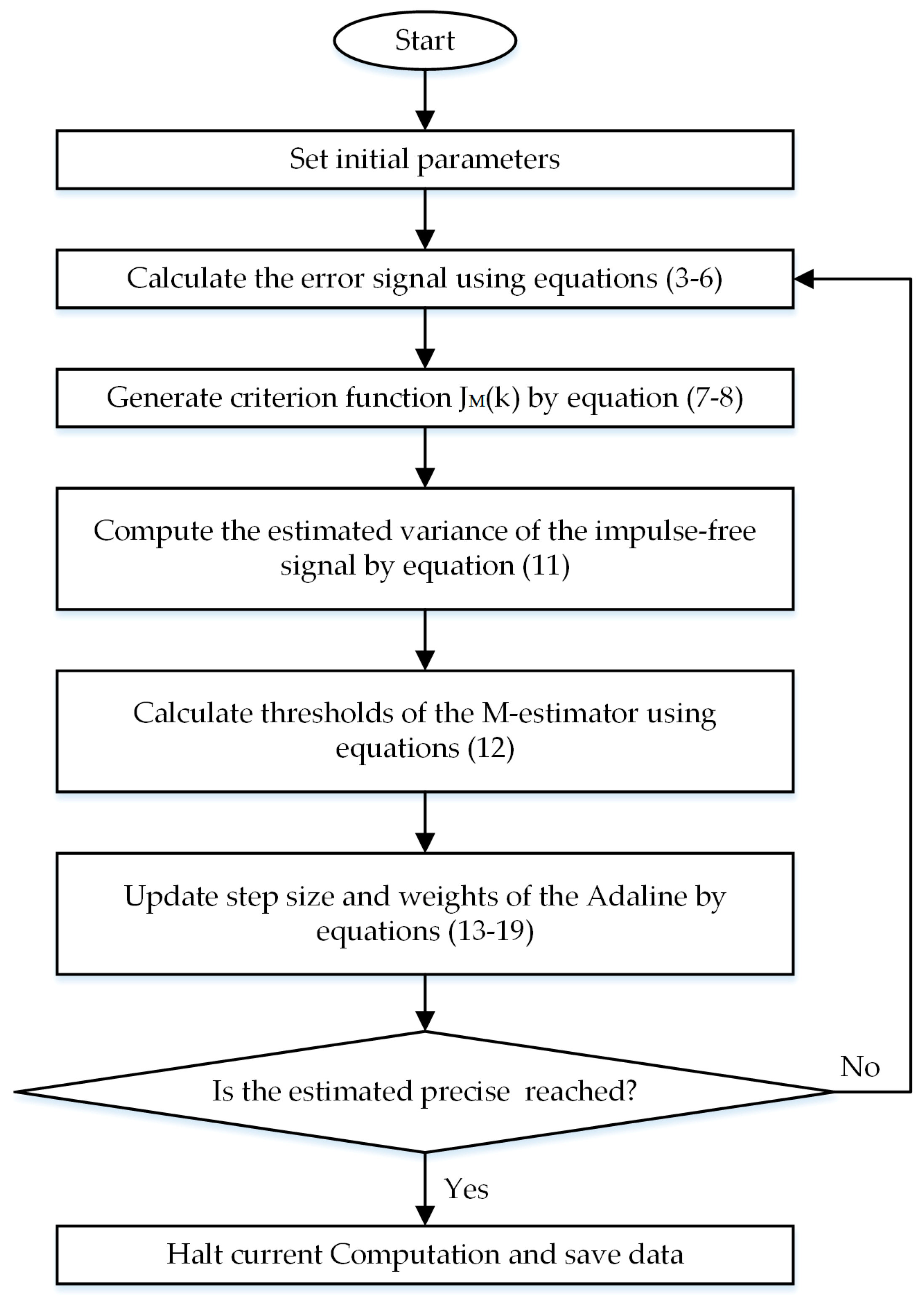
The weight is optimized by using the LMM algorithm which is a nonlinear algorithm using the error signal’s M-estimator to minimize the instantaneous criterion function $J_M(k)$. The criterion function $J_M(k)$ is expressed as:

$$J_M(k)=E\{M(e(k))\}$$

(7)

where M(.) is a robust M-estimate function that can be obtained by using Hampel’s three parts re-descending function which is expressed as:

$$M(e(k))=\left\{\begin{array}{ll}\frac{e^2(k)}{2}& 0<\left|e(k)\right|<t_1\\ t_1\left|e(k)\right|-\frac{{h_1}^2}{2}& t_1\le \left|e(k)\right|<t_2\\ \frac{h_1}{2}(h_2+h_3)-\frac{{h_1}^2}{2}+\frac{h_1}{2}\frac{{(\left|e(k)\right|-h_3)}^2}{h_2-h_3}& t_2\le \left|e(k)\right|<t_3\\ 0& t_3\le \left|e(k)\right|\end{array}\right\}$$

(8)

$$S(e(k))=\frac{\partial (M(e(k)))}{\partial (e(k))}$$

(9)

where $S(e(k))$ is called the score or influence function as what is shown in Equation (10).

$$S(e(k))=\left\{\begin{array}{ll}e(k)& 0<\left|e(k)\right|<t_1\\ t_1\mathrm{sgn}(e(k))& t_1\le \left|e(k)\right|<t_2\\ [\left|e(k)\right|-t_3]\frac{t_1}{t_2-t_3}\mathrm{sgn}(e(k))& t_2\le \left|e(k)\right|<t_3\\ 0& t_3\le \left|e(k)\right|\end{array}\right\}$$

(10)

where t₁, t₂ and t₃ are thresholds which are used to control the impulse-suppressing degree and can be determined by estimating the variance of the impulse free signal. These threshold parameters can be estimated as [17]:

$${\widehat{\delta }}^2(k)=C_1{\widehat{\delta }}^2(k-1)+(1-C_1)C_{2}med(e{(k)}^2,e{(k-1)}^2,\dots e{(k-L_w+1)}^2)$$

(11)

$$\{\begin{array}{l}{t}_1=1.96\delta (k)\\ t_2=2.24\delta (k)\\ t_3=2.57\delta (k)\end{array}$$

(12)

where $\widehat{\delta }(k)$ is the estimated value of the variance of the impulse-free signal. $C_1=1.483(1+5/(L_w-1\left)\right)$ ($C_1\le 1$) and $C_2$ ($2<C_2<3$) are the active forgetting factor and the modifying factor respectively. $L_w$ represents the length of the estimated window. Apparently, the stability and the tracing performance of LMM depend on these parameters.

When the criterion function $J_M(k)$ reaches the minimum value, the weight gets its optimized value. The first derivative of the criterion function can be given as:

$$\frac{\partial }{\partial {\omega }_{ai}(k)}{J}_M(k)=\frac{\partial }{\partial {\omega }_{ai}(k)}M(e(k))=-S(e(k))X_{ai}(k)$$

(13)

$$\frac{\partial }{\partial {\omega }_{bi}(k)}{J}_M(k)=\frac{\partial }{\partial {\omega }_{bi}(k)}M(e(k))=-S(e(k))X_{bi}(k)$$

(14)

The updating equations of the Adaline neural network’s weights are shown as:

$${\omega }_{ai}(k+1)={\omega }_{ai}(k)+{\mu }_{ai}(k)(-\frac{\partial }{\partial {\omega }_{ai}(k)}{J}_M(k))$$

(15)

$${\omega }_{bi}(k+1)={\omega }_{bi}(k)+{\mu }_{bi}(k)(-\frac{\partial }{\partial {\omega }_{bi}(k)}{J}_M(k))$$

(16)

Substituting Equations (13) and (14) into Equations (15) and (16), the weight updating equation using Adaline-LMM algorithm can be given as:

$${\omega }_{ai}(k+1)={\omega }_{ai}(k)+{\mu }_{ai}S(e(k))X_{ai}(k)$$

(17)

$${\omega }_{bi}(k+1)={\omega }_{bi}(k)+{\mu }_{bi}S(e(k))X_{bi}(k)$$

(18)

where ${\mu }_{ai}$, ${\mu }_{bi}$ represent variable weight updating step sizes which can be updated as:

$${\mu }_{ai}={\mu }_{bi}=\mu ={0.25}^{\frac{i}{50}}$$

(19)

where i is the number of iterations. If $\mu <0.0001$, $\mu =0.0001$.

When the Adaptive neutral network has been trained, the error signal is very close to 0. At the time when the output of the network equals to the system’s output, the weight could not be adjusted. i.e., the ultimate weight vector is the Fourier coefficient vector of the signal. The ultimate weight vector can be given as:

$${\omega }_a=[{\omega }_{a1},{\omega }_{a2},\cdots ,{\omega }_{aN}]$$

(20)

$${\omega }_b=[{\omega }_{b1},{\omega }_{b2},\cdots ,{\omega }_{bN}]$$

(21)

Due to Equations (20) and (21), the ith harmonic’s amplitude and phase can be computed by:

$$A_i=\sqrt{{({\omega }_{ai}(k))}^2+{({\omega }_{bi}(k))}^2}$$

(22)

$${\phi }_i={\tan }^{-1}(w_{bi}(k)/w_{ai}(k))$$

(23)

In summary, the adopted least mean M-estimate algorithm can be described by a flow chart which is shown in Figure 5.

4. Simulation Results

The real-time and precision identification performance of the proposed Adaline-LMM algorithm is initially tested by simulation using MATLAB/SIMULINK. The simulation input is:

$$\begin{array}{ll}a\left(k\right)& =3\sin \left(\omega k+1.2\right)+0.6\sin \left(2\omega k+0.9\right)+0.5\sin \left(3\omega k+0.7\right)+0.4\sin \left(4\omega k+0.5\right)\\ & +0.3\sin \left(5\omega k+0.4\right)+0.2\sin \left(6\omega k+0.3\right)\end{array}$$

(24)

Apparently, there are 6 harmonics whose frequencies are the integral multiple of the fundamental frequency. Its sampling frequency is 1000 Hz. The fundamental frequency is 3 Hz. The optimum values of constant parameters such as $C_1$, $C_2$, are 0.995, 2.157 respectively. $L_w$ is set as 12 because there are 6 harmonics existing in the simulation input. The initial values of both ${\omega }_{ai}(k)$ and ${\omega }_{bi}(k)$ are chosen as 0.018.

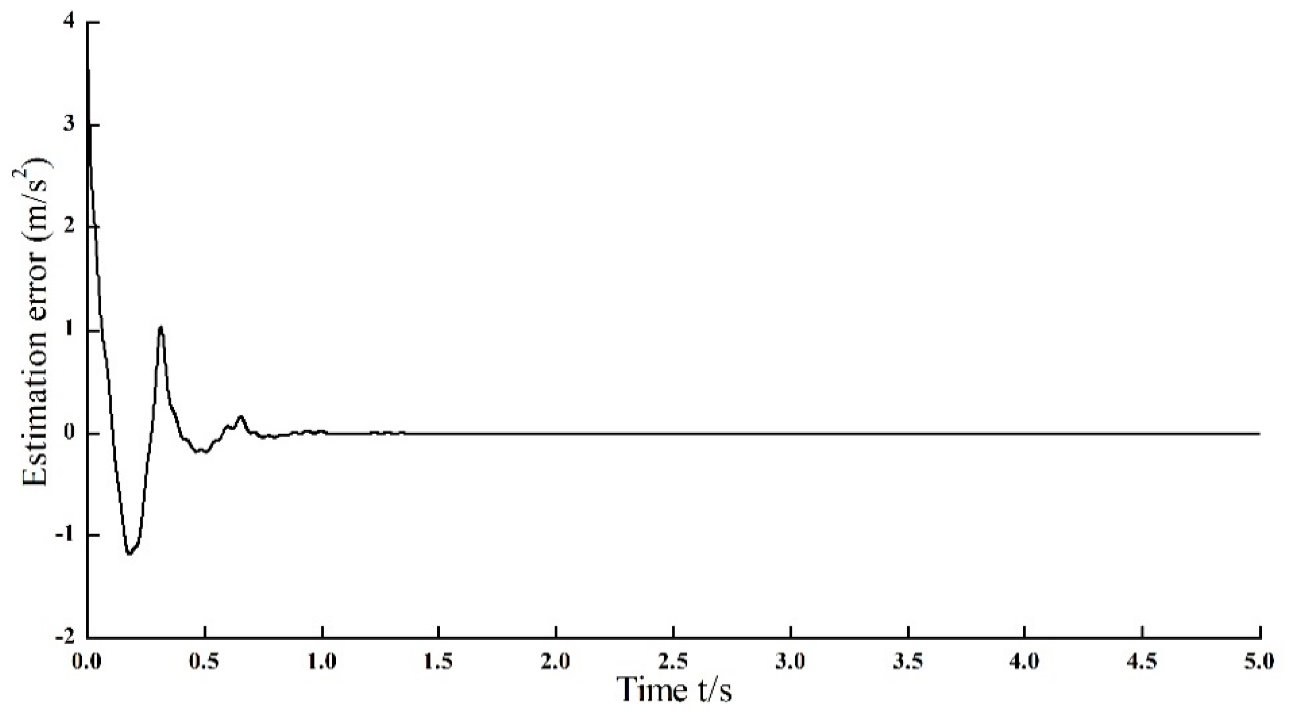
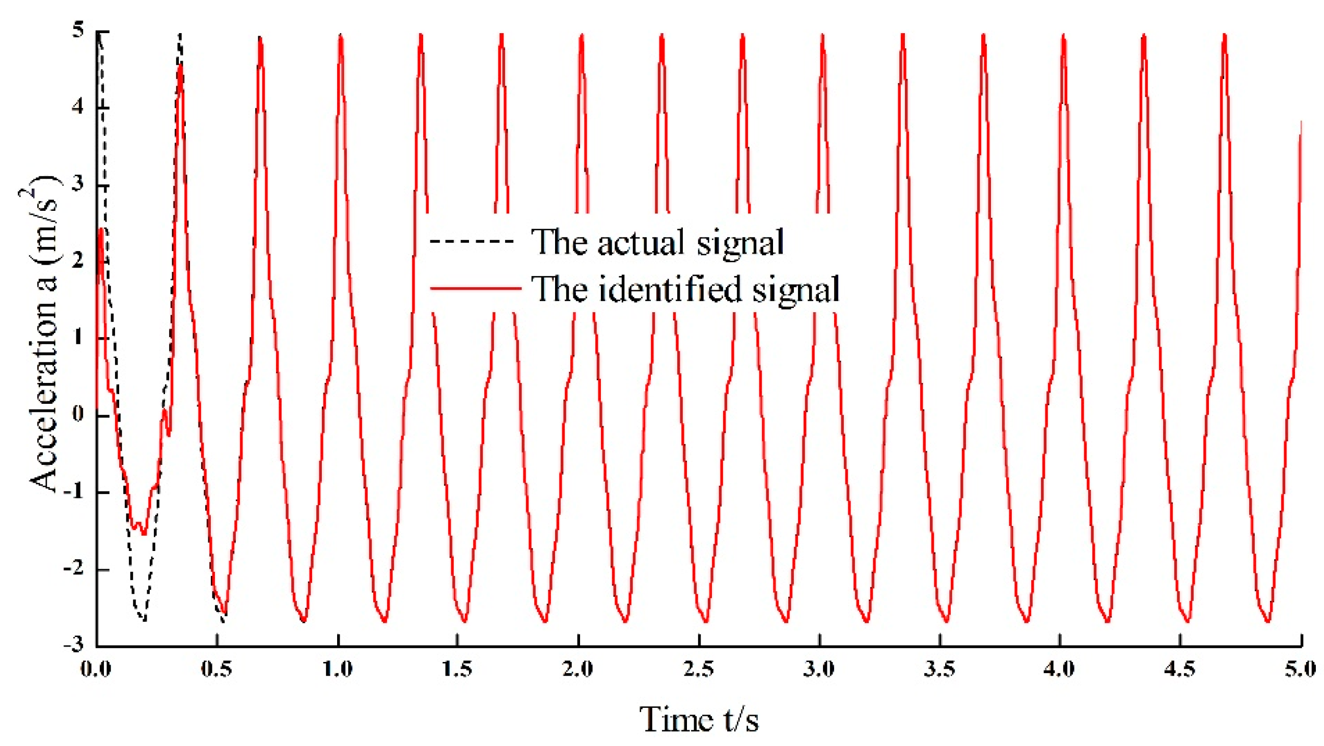
From the error plot in Figure 6, it is noted that the estimation error is converging to nearly zero within 1s, in spite of large fluctuation existing in the initial stage of harmonic identification. Figure 7 contains two different kinds of signals, both the actual signal denoted by dashed line and the identified signal denoted by red line. Although the estimation error is quite large originally, it is noted that the identified signal is well converged to the actual signal within 0.7 s which means both the amplitude and the phase of each harmonic are precisely estimated.

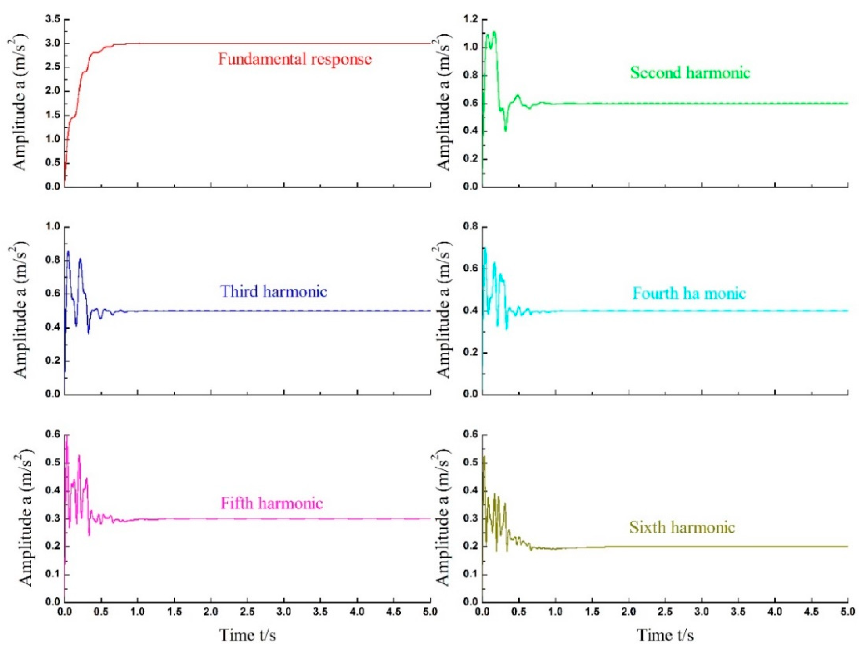
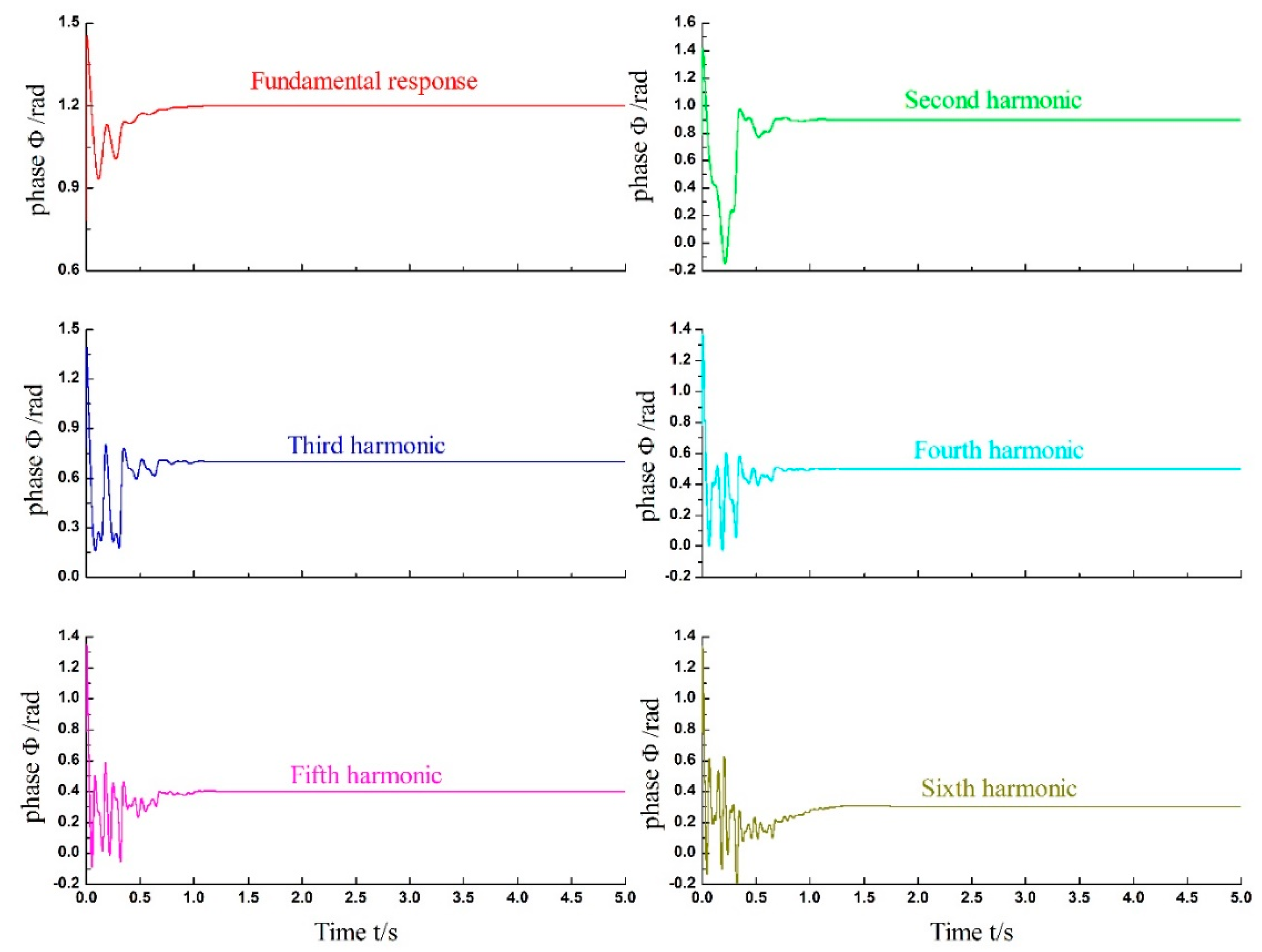
The estimation amplitude and phase of each identified harmonic are separately shown in Figure 8 and Figure 9, and the result of contrast between the estimated values and the set values is showed in

Table 3. The result of contrast between the estimated values and the given values.

Harmonic Order	Set Values		Estimated Values (LMM)
	Amplitude (m/s2)	Phase (rad)	Amplitude (m/s2)	Phase (rad)
Fundamental response	3	1.2	2.999999	1.199999
Second harmonic	0.6	0.9	0.599999	0.899999
Third harmonic	0.5	0.7	0.500000	0.700000
Fourth harmonic	0.4	0.5	0.399999	0.500000
Fifth harmonic	0.3	0.4	0.300000	0.400000
Sixth harmonic	0.2	0.3	0.199999	0.299999

. At the initial stage of the harmonic identification, there are relatively large fluctuation. But both amplitudes and phases of all the harmonics are converging to their specific values which are exactly the same as what the simulation input signal contains originally, i.e., the amplitude and phase of each harmonic are precisely estimated by using Adaline-LMM algorithm. Besides, harmonics can be directly identified and its results are shown in Figure 10.

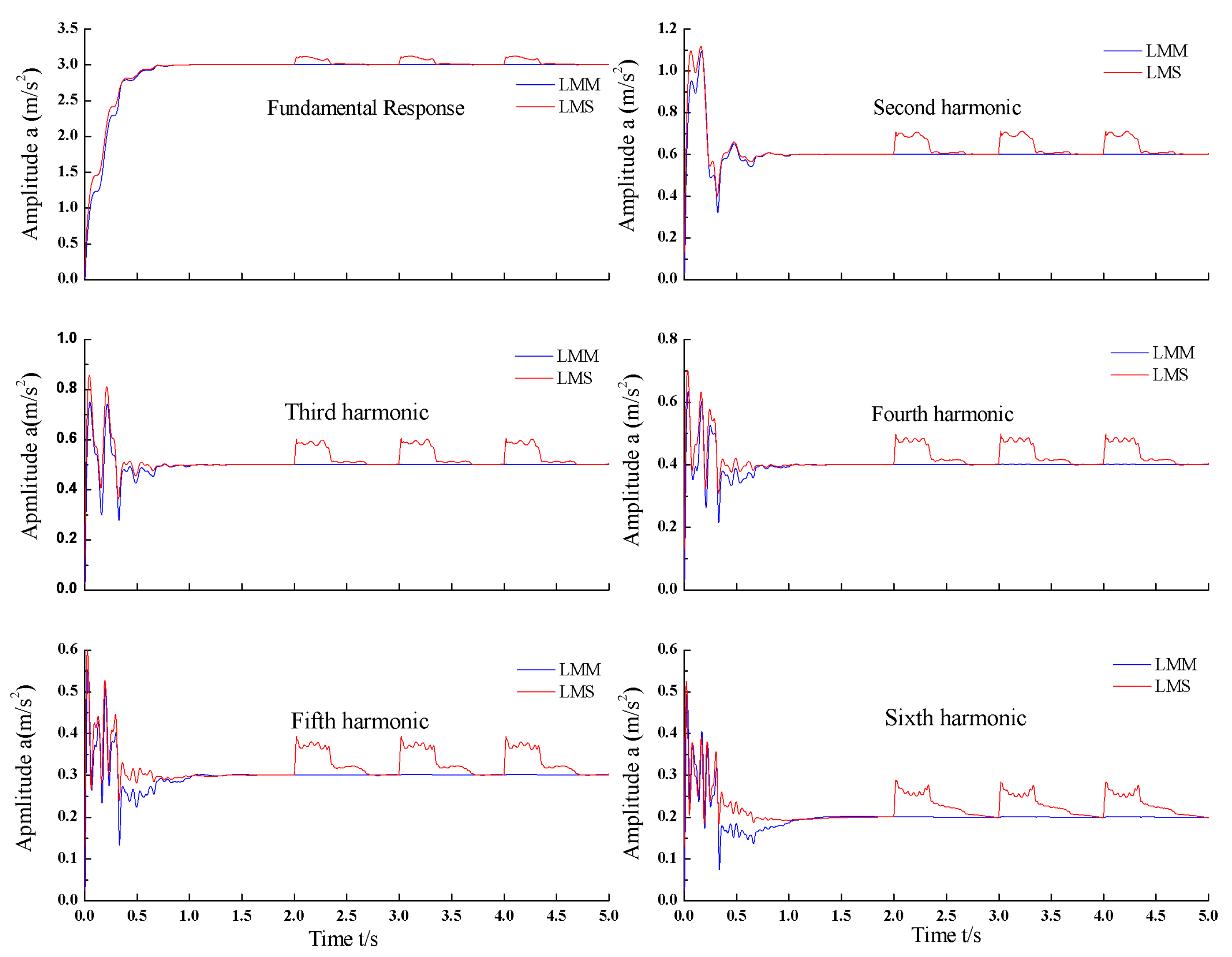
To validate the impulse noise suppression ability of the Adaline-LMM algorithm in harmonic identification, impulse noises (SNR: 15 dB) are independently added into the simulation input signal and the appearing time of these are fixed at 2 s, 3 s and 4 s during the simulation. The amplitudes are set as 0.8891. For confirming the advantage of LMM on impulse noise suppression objectively, as a contrast, LMS algorithm is also used in harmonic identification when the input signal is contaminated by the impulse noise. Other parameters are set as the same with the above. According to the results which is shown in Figure 11, the estimation error has large fluctuation at the time when impulse noise is acted in the input signal and there still has small oscillation after 2.5 s, 3.5 s and 4.5 s (the action time of the impulse noise are 2 s, 3 s and 4 s), but the estimation error is converged to zero and the error oscillation does emerge during the whole identification time.

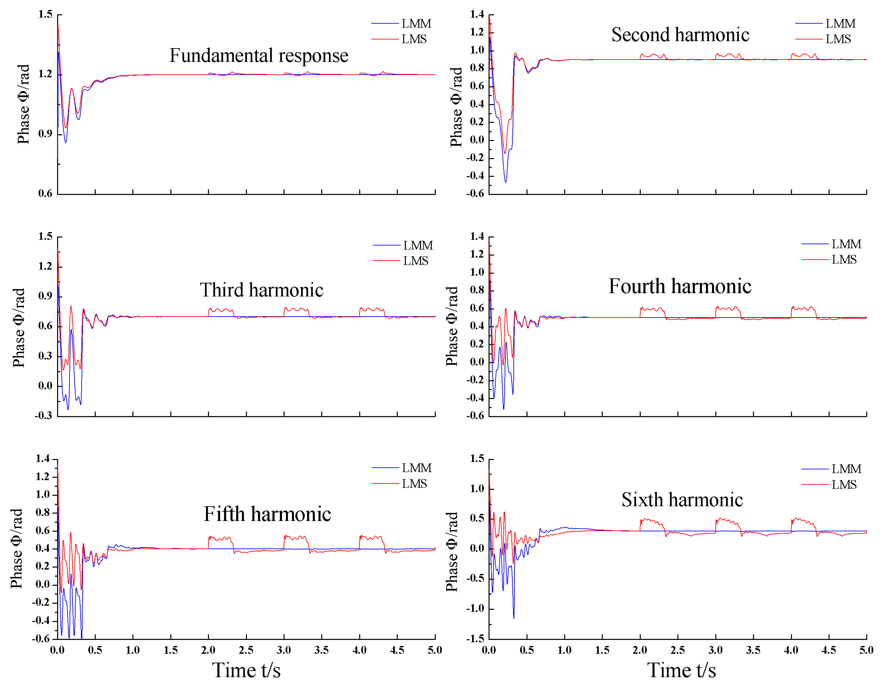
For simplicity in visualizing the merits of LMM, the identification results, both amplitude and phase of each harmonic, are separately shown in Figure 12 and Figure 13. It is noted that the identification amplitudes and phases are not stable and easily affected by the impulse noise, which is not allowed in the acceleration harmonics identification for an electro-hydraulic servo shaking table. On the contrary, the amplitudes and phases estimated results by using LMM algorithm are more stable and not influenced by impulse noises. That is, unlike the LMS algorithm, the LMM can detect and ignore the impulse noise and provide a more stable and precise harmonic identification performance.

5. Experiment Results

For validating the effectiveness of the proposed algorithm for harmonic identification further, the real experiment is designed to test its identification precision. The initial values of both ${\omega }_{ai}(k)$ and ${\omega }_{bi}(k)$ are chosen as 0.05. Its sampling frequency is also 1000 Hz. 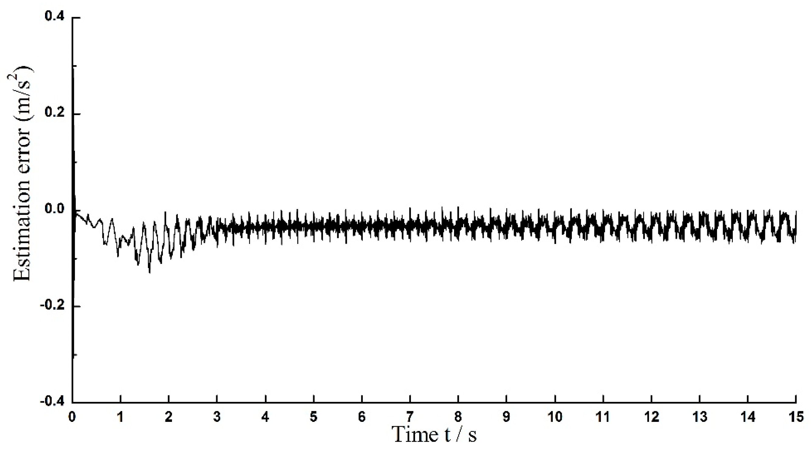During the experiment, the Adaline-LMM parameters are kept as the same as the simulation except $L_w$ which is set as 16 because there are eight harmonics, including fundamental response, existing in the system response and C₂ which is set as 1.071. 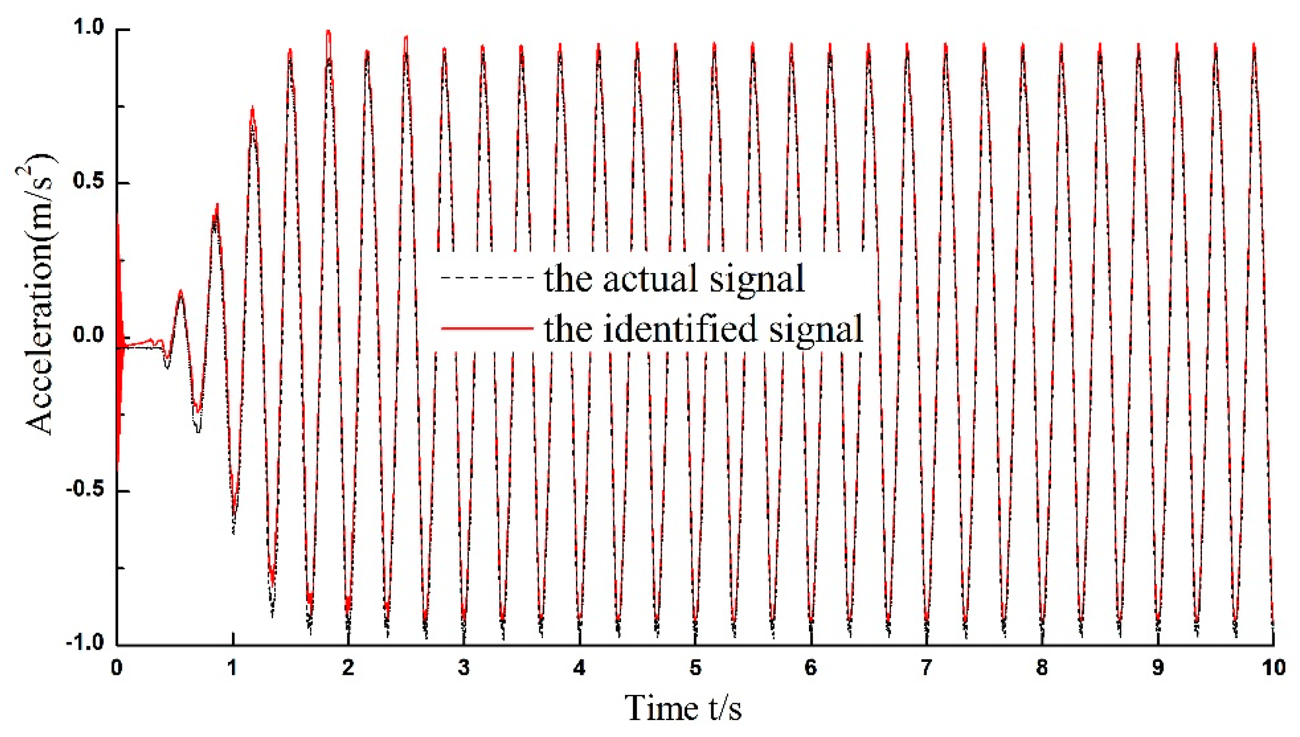The estimation error is displayed in Figure 14 which is used to demonstrate the estimation accuracy. It is noted that the estimation error fluctuates largely at the beginning of the identification but it is rapidly converged to a relative small range (within 0.08) after 2 s. There are two different lines, the dashed one and the red line contained in Figure 15. The dashed line is the actual system response and the red line presents the identified signal. Initially, the red line has a wide fluctuation, however, after the Adaline-LMM algorithm has been trained, the identified signal is ultimately well converged to the actual signal within 2 s. That is, the identified signal matches the actual signal very well and the harmonic identification precision of the proposed algorithm is rather successful.

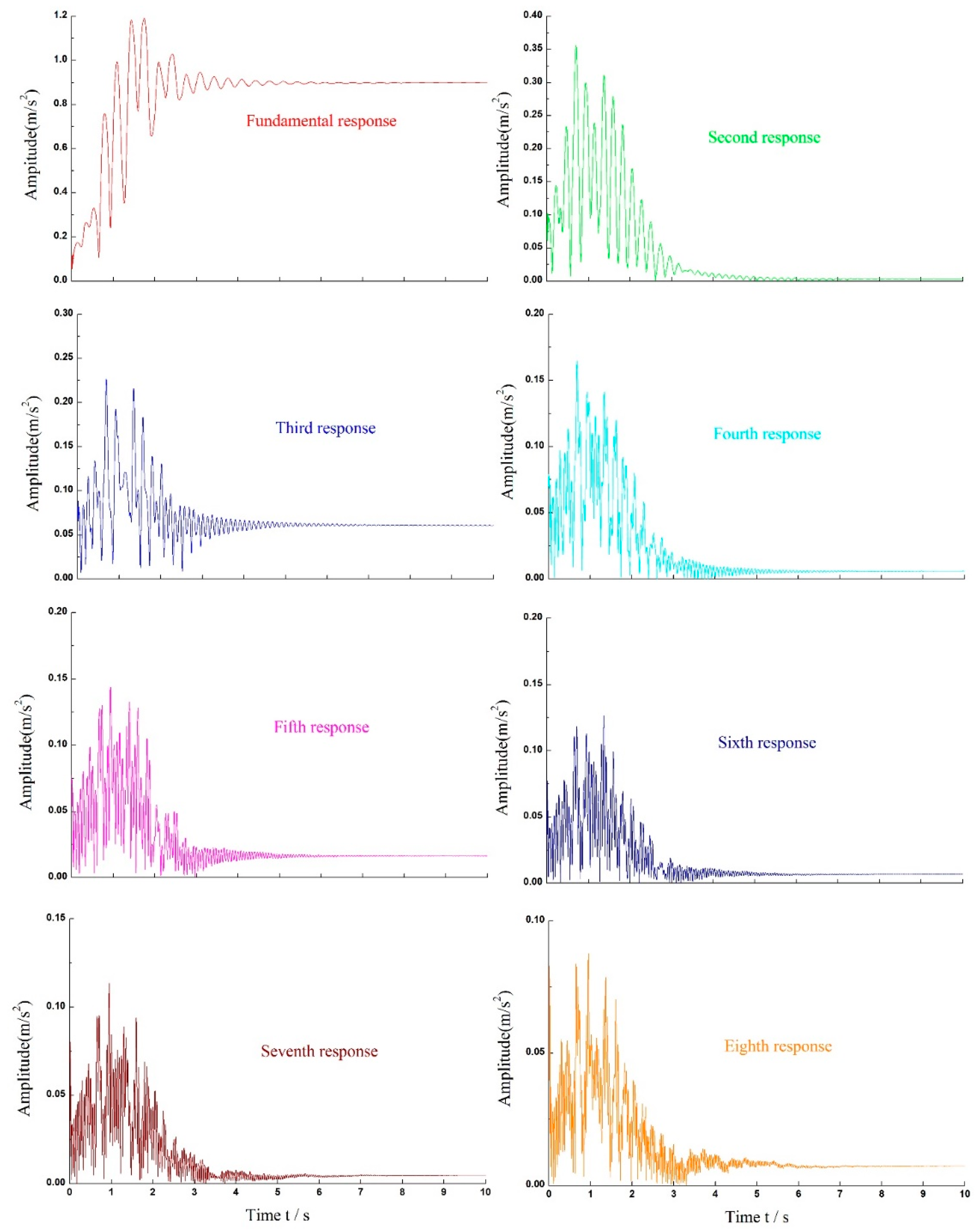
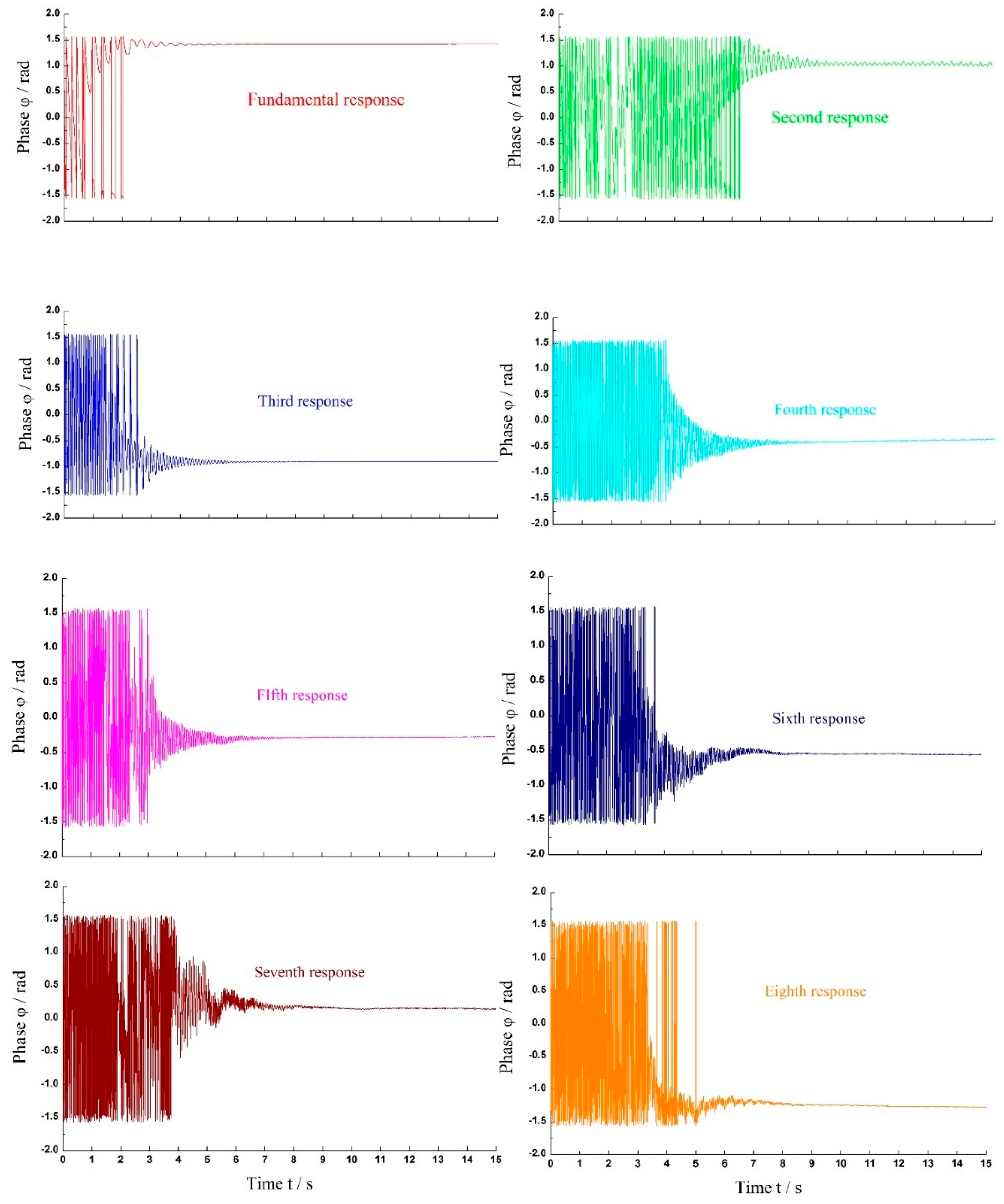
The estimation amplitude results are displayed in Figure 16. It is noted that all amplitude values are converged to determined values which match well with the FFT-computed values shown in Table 2. That is, all amplitude values are precisely identified. From the estimation phase results shown in Figure 17, large fluctuations exist within initial 2 s, but they tend to be steady after around 4 s. However, there are still minor variations of the estimation phase existing in the second harmonic. 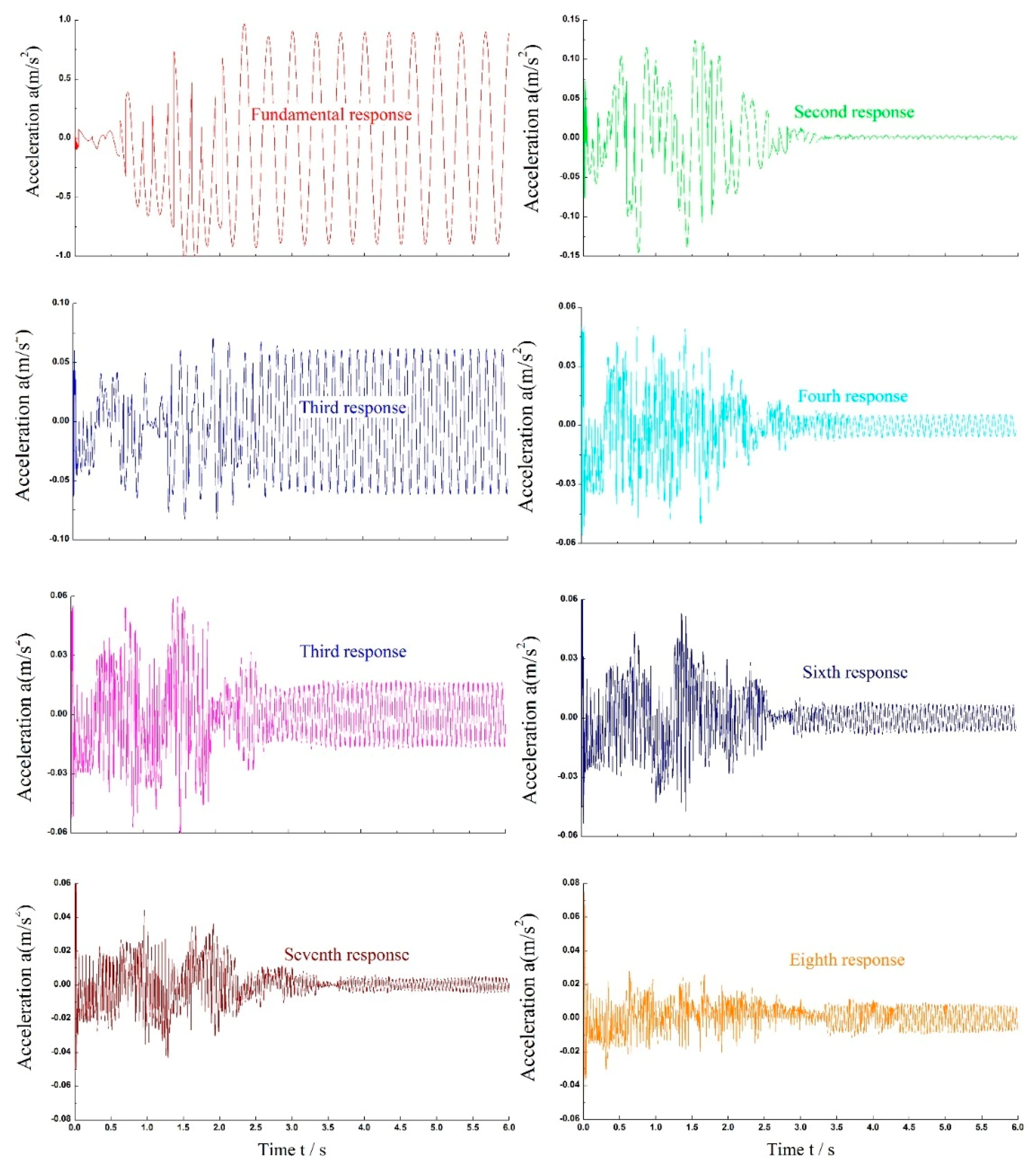Also, from both Figure 16 and Figure 17 we can see that the convergence speed of the estimated amplitude and phase values of the fundamental response are faster than other seven harmonics. Certainly, all of the harmonics can also be directly estimated online, and their waveforms are shown in Figure 18. From Figure 18, it can be seen that almost all the harmonics contained in the system response are well estimated except second harmonic which means that the identification results can be used for further research, such as harmonic compensation and cancellation.

6. Conclusions

When the electro-hydraulic servo shaking table was excited by a sinusoidal signal, the system response contained high order harmonics due to many nonlinear elements existing in this shaking table. For identifying each harmonic, both the amplitude and the phase, a nonlinear adaptive algorithm based on a single layer ADALINE and LMM which was used to adjust the weights of the Adaline was proposed. Both the simulation and experimental results showed that the proposed algorithm was able to identify the amplitude and phase of each harmonic online, and its real-time performance and precision had been proved to be satisfied.

Besides, the proposed ADALINE-LMM algorithm exhibited other characteristics like great tracing precision, fast convergence and simple algorithm construction. The most obvious advantage of this algorithm was that it can effectively detect and ignore the impulse noises during the identification process which was verified by the simulation results. The simulation result showed that Compared with the LMS algorithm, the LMM algorithm was able to provide the more stable harmonic identification performance when the signal response was contaminated by impulse noise. Furthermore, the results using the proposed harmonic identification scheme deserved to be studied further because they are not only useful for harmonic identification, but also for harmonic compensation and cancellation.