Health Monitoring for Balancing Tail Ropes of a Hoisting System Using a Convolutional Neural Network

Abstract

With the arrival of the big data era, it has become possible to apply deep learning to the health monitoring of mine production. In this paper, a convolutional neural network (CNN)-based method is proposed to monitor the health condition of the balancing tail ropes (BTRs) of the hoisting system, in which the feature of the BTR image is adaptively extracted using a CNN. This method can automatically detect various BTR faults in real-time, including disproportional spacing, twisted rope, broken strand and broken rope faults. Firstly, a CNN structure is proposed, and regularization technology is adopted to prevent overfitting. Then, a method of image dataset description and establishment that can cover the entire feature space of overhanging BTRs is put forward. Finally, the CNN and two traditional data mining algorithms, namely, k-nearest neighbor (KNN) and an artificial neural network with back propagation (ANN-BP), are adopted to train and test the established dataset, and the influence of hyperparameters on the network diagnostic accuracy is investigated experimentally. The experimental results showed that the CNN could effectively avoid complex steps such as manual feature extraction, that the learning rate and batch-size strongly affected the accuracy and training efficiency, and that the fault diagnosis accuracy of CNN was 100%, which was higher than that of KNN and ANN-BP. Therefore, the proposed CNN with high accuracy, real-time functioning and generalization performance is suitable for application in the health monitoring of hoisting system BTRs.

1. Introduction

A mine’s hoisting system is the only way to connect the underground with the ground and is known as the “throat” of the mine [1,2]. It is a mechatronics-hydraulics-integrated system (comprising a driving friction pulley, hoisting ropes, head sheaves, containers, balancing tail ropes, etc.) [3], including complex dynamic characteristics like inertia, flexibility, and damping in its operation. The tail rope is an important component of the hoisting system. It is set up to balance the gravity of the hoisting rope and to obtain equal moments in the mine hoisting system [3]. Hence, the working state and mechanical properties of the tail rope directly affect the safety of mine production [4].

The balancing tail ropes (BTRs) are located at the bottom of the hoisting container, which is in the dark shaft all (or most) the time [5]. Research and production experience show that the causes of the BTR faults (disproportional spacing, twisted rope, broken strand, broken rope, etc.) include operational vibration, the impact of the falling ore, wind in the shaft, corrosion, etc. Faults and accidents give rise to many problems, such as influencing the system stability, breaking shaft equipment, threatening the lives of mine workers and causing production to stop. However, the traditional maintenance of BTRs only depends on workers with handheld flashlights, which is difficult, inefficient, and unsafe. The frequent fault occurrences of BTRs pose a serious threat to the safe operation of the hoisting system. For example, in the main shaft hoisting system of the Tong-ting Coal Mine Enterprise, tail ropes were broken or damaged five times during 1989–1998. Its tail ropes have been replaced ten times because of faults, resulting in a serious loss of manpower, material resources, and financial resources. The tail ropes in the main shaft of the Bei-ming-he Iron Mine Enterprise broke and fell on 14 February 2011, causing shaft damage, and resulting in substantial economic losses. Therefore, health monitoring for identifying faults in BTRs and taking appropriate measures to eliminate the faults would be beneficial to the safety and efficiency of hoisting systems.

A variety of research focusing on health monitoring and fault diagnosis methods in hoisting systems has already been conducted. For instance, Jiang et al. [6] proposed a condition-monitoring method based on variational mode decomposition and support vector machine via vibration signal analysis to facilitate accurate fault monitoring of the abnormal lifting load of a mine hoist. Chang et al. [7] also proposed a mine hoist fault diagnosis method using a support vector machine. Henao et al. [8] theoretically and experimentally analyzed the stator current and load torque of a three-phase induction machine in a hoisting winch system and realized the fault detection of the wire rope. In addition, an application of a probabilistic causal-effect model based on the artificial fish-swarm algorithm for fault diagnosis in mine hoists was proposed by Wang [9]. However, there are few studies on the health monitoring and fault diagnosis of hoisting system BTRs. Chang [5] designed an online monitoring and early warning system for the hoist balance tail ropes based on machine vision. The system extracts the image feature parameters with integral projection and Hu invariant moment, and the pattern recognition is ultimately used to identify the fault information. The method used by Chang needs complex image processing and manual feature extraction in the early stage, which has the disadvantages of low efficiency and poor accuracy when handling big data, and is difficult to meet the requirements of real time and accuracy. At the same time, it is unable to cover the entire feature space because there are so few samples in the dataset, meaning that the model’s generalization performance is poor. Hence, with the growing security requirements of hoisting systems, the traditional methods will be difficult to achieve high accuracy, real time and generalization performance.

Since 2006, deep learning (DL) [10] has become a rapidly growing research direction [11]. As an important DL algorithm, the convolutional neural network (CNN), has recently become a research hotspot in the field of pattern recognition [12], and is widely used in speech recognition [13], image recognition [14,15,16], behavior detection [17,18], text classification [19] and more. In the field of image recognition, the original image can be put into the CNN directly without complicated pretreatment. Additionally, owing to CNNs’ local receptive field, weight sharing, and down sampling, it is highly invariant to image information in the deformation of translation, inclination, scaling, and so on. CNNs have been widely applied because of the aforementioned advantages [20].

Considering the capability of DL to address big data and learn high-level representation, it can be a powerful and effective method for machine health monitoring systems (MHMS) [11]. At present, in the field of MHMS, the CNN-based health monitoring and fault diagnosis of mechanical systems are still in the initial stage of exploration. Chen et al. [21] used a CNN to realize gearbox fault detection and classification. Janssens et al. [22] used a CNN to realize fault detection and recognition in the rotating machinery without expert experience. Weimer et al. [23] did a comprehensive study of different CNN configurations for automated feature extraction in industrial inspection. Ince et al. [24] successfully developed a one-dimensional (1D) CNN on raw time series data for real-time motor fault detection. Ding et al. [25] proposed a deep convolutional network for spindle bearing fault diagnosis, and they used wavelet packet energy images as the input. Abdeljaber et al. [26] also proposed a 1D CNN, which can execute damage detection and structural damage localization in real-time via normalized vibration signals. Fault diagnosis methods based on CNN have only been under development for approximately four years (2015–2018) [11], the CNN-based method is also under great demand to address these challenges. However, although DL technology has great potential, there are still few applications emerging from the research into the health monitoring and fault diagnosis of mechanical systems [27], especially in terms of hoisting systems.

Due to the important role of the hoisting system, it is rarely shutdown. Thus, the real-time monitoring of BTRs via machine vision will involve massive images (i.e., big image data). The traditional methods find it difficult to process big data, so it is very suitable to apply CNNs for the diagnosis of BTR faults. Additionally, the research in this paper has great significance because CNNs have not yet been applied in the field of health monitoring and fault diagnosis for hoisting systems’ BTRs. This paper presents the design of an online BTR monitoring system based on machine vision and a CNN, that can provide reliable fault warning information, realize the automation of BTR’ fault monitoring, and improve the safety of the mine hoisting system. The main contributions of this paper are as follows: (1) The deep learning method is introduced to the health monitoring and fault diagnosis of hoisting systems for the first time, and a CNN method is proposed that diagnoses BTR faults more accurately than k-nearest neighbor (KNN) and artificial neural network with back propagation (ANN-BP) algorithms; (2) A method of establishing a BTR image dataset that can cover the entire feature space is put forward; (3) The same framework can be applied to other health monitoring and fault diagnosis applications where machine vision and CNN are demanded.

This paper is organized as follows: the image data-driven monitoring system framework is proposed in Section 2. In Section 3, the principles are introduced and the design of the CNN structure is presented. Section 4 describes how the tail ropes monitoring dataset is built. In Section 5, the experimental design and results analysis are presented and discussed, and a comparison with other methods is made. The industrial implementation plan is proposed in Section 6, and the paper is concluded in Section 7.

2. Image Data-Driven Monitoring System Framework

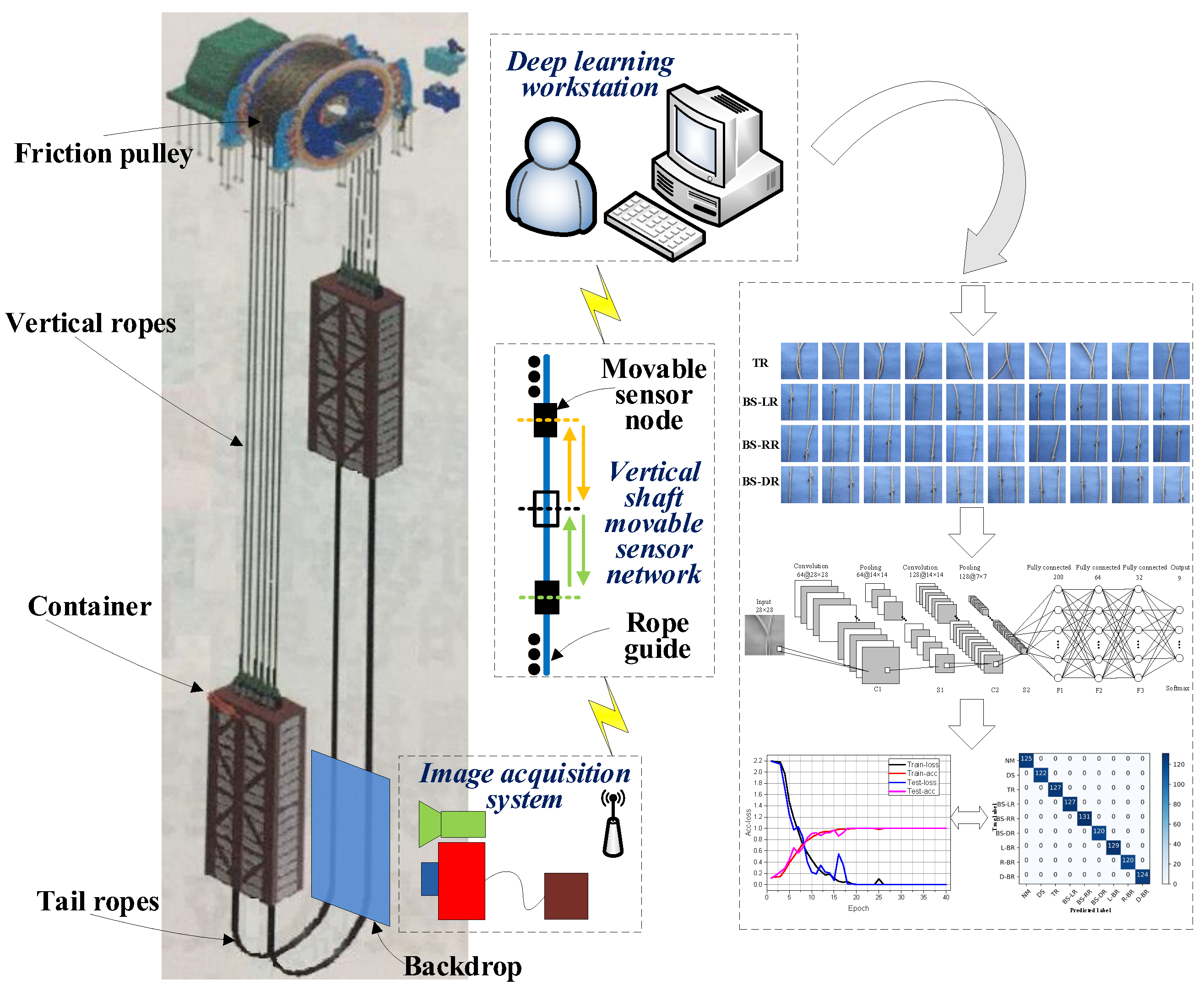
A schematic diagram of the proposed image data-driven monitoring system framework is presented in Figure 1.

The monitoring system framework is composed of three parts, including the image acquisition system, the vertical shaft movable sensor network [28] and the upper computer. The image acquisition system includes a light source, CCD (charge coupled device) cameras, an acquisition card and memory, and can realize the real-time collection of the BTRs image data. The movable sensor network transfers the collected image data to the upper computer. The upper computer is made up of one or more high-performance deep learning workstations, allowing it to achieve the deep mining of big image data features, analyze the data, and give BTR fault warnings. If the tail rope is found to be twisted, broken, or unevenly distributed, the diagnosis information will be sent out immediately so as to avoid the enlargement of the fault. Our work mainly focuses on the study of health monitoring methods. Other aspects of the system, such as the design of the hardware and software of the image acquisition system and the design of the movable sensor network, are not discussed in this paper.

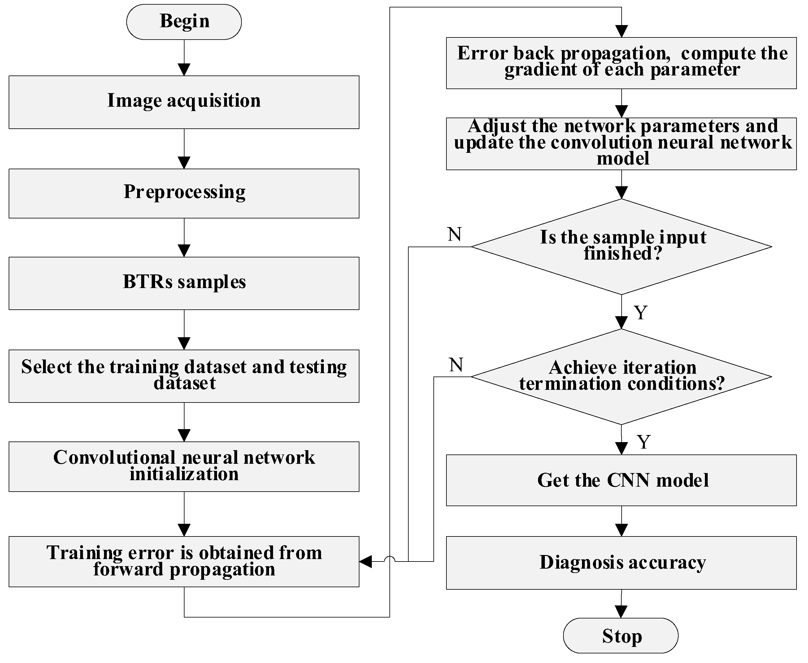
As shown in Figure 1, the proposed image data-driven framework for monitoring BTRs is developed by the following steps:

Step 1. Generate the training and testing dataset: collect the BTR image data, clean the data, and divide the processed BTR image data into training and testing datasets [29].

Step 2. Develop the model: based on the dataset, apply data-driven algorithms to develop models for predicting the BTRs’ condition [29]. To adjust and optimize the parameter settings of algorithms, the trial-and-error method [20,30] is employed.

Step 3. Model selection: compute the prediction accuracy based on the developed models, and select the most accurate one for monitoring the BTRs’ condition.

Step 4. Online monitoring: design the hardware and software of the monitoring system, and apply them to online monitoring.

3. Convolutional Neural Network

A CNN consists of an input layer, a hidden layer, a fully connected layer and an output layer, in which the hidden layer is composed of several alternating convolution layers and pooling layers. The alternating convolution and pooling layers form a sub-convolution-pooling neural network as shown in Figure 2 and the CNN comprises multiple sub-convolution-pooling neural networks [20]. The feature map of the input layer is convoluted by specific convolution kernels in the convolution layer, a bias is added, and then an output feature is obtained by an activation function, in which the commonly used activation functions are sigmoid, tanh(x), rectified linear unit (ReLU), leaky ReLU, etc. The pooling layer is a feature selection for the output feature map of the convolution layer. The fully connected layer and the output layer constitute the classifier which can be Softmax, support vector machine (SVM), etc. [31,32].

3.1. Principle and Proposed Structure

3.1.1. Principle

(1) Convolution

In the convolution layer, the feature map from the upper layer is convoluted by the convolution kernel, and then the output feature map is obtained via the activation function [33]:

$$x_j^{\ell }=f(u_j^{\ell }),$$

(1)

$$u_j^{\ell }={\displaystyle \sum _{i\in M_j}{x}_i^{\ell -1}}\ast k_{ij}^{\ell }+b_j^{\ell },$$

(2)

where $u_j^{\ell }$ is the net activation of the j channel in the convolution layer, which is obtained by summing the convolution and bias of the output feature map $x_i^{\ell -1}$ of the upper layer. $x_j^{\ell }$ is the output of the j channel of the convolution layer. f (·) is called the activation function, and it is a ReLU function in this paper. M_j represents a subset of input feature maps for computing, $k_{ij}^{\ell }$ is a convolution kernel, and $b_j^{\ell }$ is the bias item of the feature map after convoluting. For an output feature map $x_j^{\ell }$, the convolution kernel $k_{ij}^{\ell }$ corresponding to each input feature map $x_i^{\ell -1}$ may be different.

(2) Pooling

The output feature map is obtained by the down sampling layer by sampling every input feature map by the following formula:

$$x_j^{\ell }=f({\beta }_j^{\ell }\mathrm{down}(x_j^{\ell -1})+b_j^{\ell }),$$

(3)

where ${\beta }_j^{\ell }$ is the weight coefficient of the down sampling layer, and $b_j^{\ell }$ is the bias of the down sampling layer. The symbol down(·) represents the down sampling function, which calculates the sum, mean or maximum value of the pixel in the n × n region of the input feature map so that the output map is reduced by n times in two dimensions.

(3) Full connection

In the fully connected network, all two-dimensional image features are stitched into one-dimensional features as inputs to the fully connected network. The output of the full connection layer can be obtained by weighting and by the activation function:

$$x_{}^{\ell }=f(u_{}^{\ell }),$$

(4)

$$u^{\ell }=w^{\ell }{x}^{\ell -1}+b^{\ell },$$

(5)

where $w^{\ell }$ is the weight coefficient of the fully connected network, and $b_{}^{\ell }$ is the bias item of the fully connected layer.

(4) Classification

To solve the multi-classification problem, the Softmax [34] function, which is located in the last layer, is usually used. It is expressed as the probabilistic expression $p(y=j/x)$, where x is the input sample and the corresponding label is y, p is the probability of sample j. Therefore, the output will be an n-dimensional vector for a classifier with n classes and the sum of the elements in a vector is 1, as shown by Equation (6) [20,35]:

$$p(y^{(i)}=n|x^{(i)};w)=\left[\begin{array}{c}p(y^{(i)}=1|x^{(i)};w)\\ p(y^{(i)}=2|x^{(i)};w)\\ ⋮\\ p(y^{(i)}=n|x^{(i)};w)\end{array}\right]=\frac{1}{{\displaystyle {\sum }_{j=1}^n{e}^{w_j^T{x}^{(i)}}}}\left[\begin{array}{c}{e}^{w_1^T{x}^{(i)}}\\ e^{w_2^T{x}^{(i)}}\\ ⋮\\ e^{w_n^T{x}^{(i)}}\end{array}\right],$$

(6)

where w is the weight, and $w_n^T{x}^{(i)}$ are the inputs of the Softmax layer. The term $1/{\displaystyle {\sum }_{j=1}^n{e}^{w_j^T{x}^{(i)}}}$ normalizes the distribution, so that it sums to 1 [20]. In the training process, the optimization algorithm is used to minimize the loss function to complete the network training. The loss function $J(\theta )$ is defined by Equation (7) [35]:

$$J(\theta )=-\frac{1}{m}\left[{\displaystyle \sum _{i=1}^m{\displaystyle \sum _{j=1}^{n}1}\left\{y^{(i)}=j\right\}\log \frac{e^{w_j^T{x}^{(i)}}}{{\displaystyle {\sum }_{l=1}^n{e}^{w_l^T{x}^{(i)}}}}}\right],$$

(7)

where $1\left\{y^{(i)}=j\right\}$ is an indicator function that always returns 1 or 0, which means that when a predicted class of the ith input is true for class j, the result is 1; otherwise, the result is 0.

(5) Regularization

The research [36,37] shows that if the network model performs excellently in the training dataset but has difficulty in obtaining a satisfactory accuracy on the testing dataset, the overfitting phenomenon appears in the model. This phenomenon can be avoided by using regularization technology to restrain the complexity of the model. The commonly used regularization technologies are L₂ regularization, L₁ regularization and dropout. In this paper, we add the L₂ regularization term to the fully connected layer. The L₂ regularization term is in the form of:

$$L_2=\frac{1}{2}\lambda {\Vert \omega \Vert }_2^2,$$

(8)

where $\omega$ is the network layer parameter to be regularized, and $\lambda$ controls the size of the regularization item. Larger values of $\lambda$ will constrain the model complexity to a large extent.

3.1.2. Structural Design

The CNN structure designed for the health monitoring of BTRs is shown in Figure 3, and the configurations of the convolution, pooling, and fully connected layers are listed in

Table 1. The configurations of the convolution, pooling, and fully connected (FC) layers.

Layer	Parameters Information	Variables	Input Data Dimension	Output Data Dimension
Conv1	64 convolution kernels with 3 × 3, stride is 1	640	28 × 28 × 1	28 × 28 × 64
Pool1	Pooling size 2 × 2, stride is 2	0	28 × 28 × 64	14 × 14 × 64
Conv2	128 convolution kernels with 3 × 3, stride is 1	73,856	14 × 14 ×64	14 × 14 × 128
Pool2	Pooling size 2 × 2, stride is 2	0	14 × 14 × 128	7 × 7 × 128
FC1	200 nodes	1,254,600	1 × 6272	1 ×200
FC2	64 nodes	12,864	1 × 200	1 × 64
FC3	32 nodes	2080	1 × 64	1 × 32

.

The input feature map is grayscale with a size of 28 × 28. The hidden layer is composed of two convolution layers and two pooling layers, in an alternating arrangement. The number of convolution kernels of the first and second convolution layers is 64 and 128, respectively (with a size of 3 × 3). Before convoluting, with the “same” padding operation, the convolution results at the boundary are preserved so that the output shape is the same as the input shape. The pooling layer uses maximum sampling, (i.e., finding the maximum value in the 2 × 2 region of the feature map). The fully connected layer is set to three layers, with each layer having 200, 64 and 32 neurons, respectively. The ReLU function is chosen as the activation function of the convolution layers and fully connected layers. The output layer selects the Softmax classifier. To prevent overfitting, we use L₂ regularization to process the fully connected layer F1.

3.2. Algorithm Flow and Experimental Environment

Before the convolutional neural network is trained and tested, the image data are collected (through the CCD camera), preprocessed (e.g., scaling, graying, etc.), and divided (via the hold-out method). The algorithm flow chart is shown in Figure 4, it involves two parts, including the forward propagation of the data and the reverse propagation of the error [32]. Firstly, the training parameters of the network are set, the weight and bias of the network are initialized, and then the input feature map processed by the convolution layer, the pooling layer and the fully connected layer is transmitted to the output layer. During this process, the output of each layer is the input of the next layer. Then, the error between the actual output and the expected output is reversely transmitted using the back propagation (BP) algorithm, layer by layer. Next, this error is allocated to each layer, and the weight and bias of the network are adjusted until the convergence condition is satisfied, thus realizing the effective supervised training of the network.

The experimental environment is described in

Table 2. The experimental environment.

Hardware Environment	Software Environment
CPU: Intel Core i5-6200U 2.40 GHz Memory: 8.00 GB	System: Windows 10, ×64 Development tool: Keras (Theano)

.

4. Dataset Description and Establishment

The establishment of the dataset is complex, and the richness and accuracy of the dataset have a direct influence on the recognition ability and generalization performance of the network. In this section, we first describe the data (i.e., the tail rope failure categories, forming reasons, and expression forms). Then, based on the data description, we establish a dataset that covers all the features.

4.1. Data Description

In the hoisting system, the states of BTRs basically include normal, disproportional spacing, twisted rope, defect, and broken rope. The disproportional spacing is caused by unstable factors in the hoisting system, such as mechanical vibration, wind-induced vibration, etc., which is the precondition of twisted rope. The twisted rope fault occurs when the hoisting system is very unstable. In this paper, the collision contact of the two ropes is also classified as a twisted rope-type fault. The twisted rope-type fault is a serious fault that causes the instability in the hoisting system and produces broken rope or downtime, so it should be avoided. Defects include wear, broken wire, broken strand, and rust, among which, a broken strand, the precondition of a broken rope, is the most serious defect. Because the broken rope directly leads to the instability of the hoisting system or even accidents, we should try to avoid it.

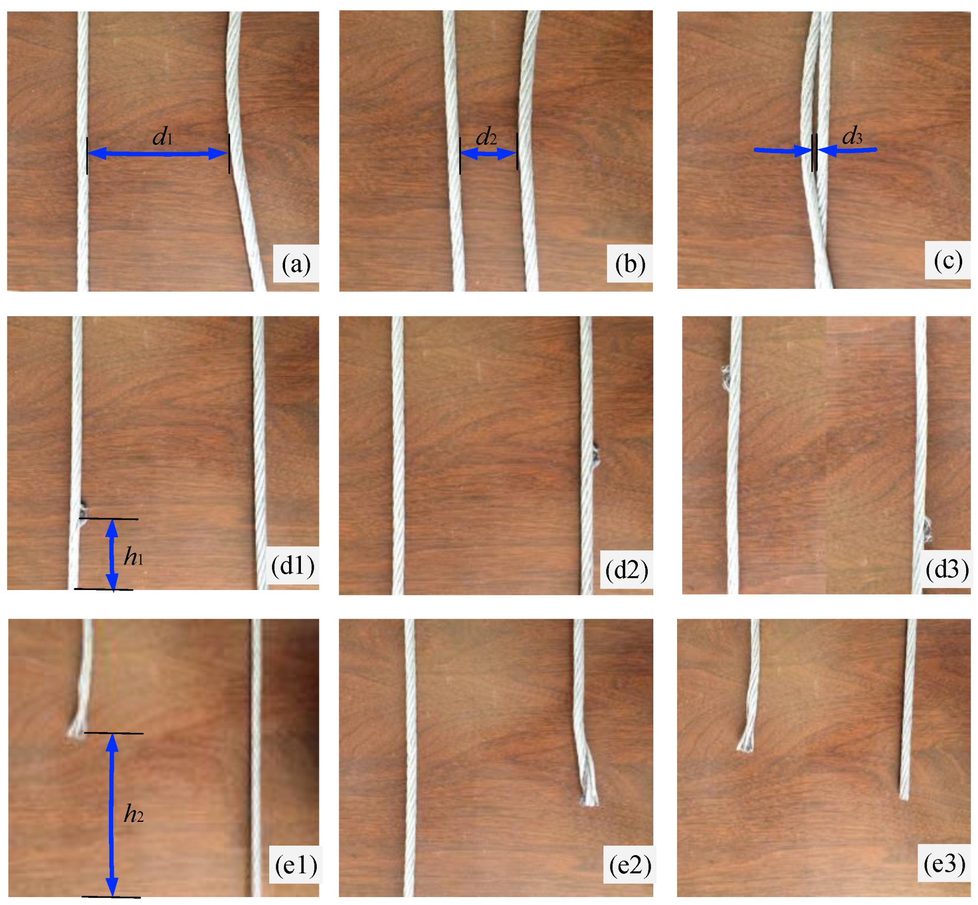
The measure of setting separate woods (using wood to separate each tail rope) has been adopted in order to prevent the collision of the BTRs, but the separate woods tend to damage the BTRs by scratching or pulling, which aggravates the wear and failure of the BTRs. The tail rope is in a state of free overhanging in the shaft, is subjected to random vibrations and external excitation, and its attitude is difficult to estimate. Therefore, according to the actual production situation, we use the empirical method to build up the BTRs’ state dataset with the whole feature space as far as possible. The image dataset in this paper is made up of five typical feature states, namely, normal (a), disproportional spacing (b), twisted rope (c), broken strand (d) and broken rope (e), as shown in Figure 5.

It should be noted that the distance of normal (a) here is defined as being greater than 3/4 of the normal distance (the distance between the tail ropes under stationary state). Disproportional spacing (b) is defined as a distance less than 1/2 of the normal distance between the two ropes. Twisted rope (c) is defined as a variety of forms in which two ropes get entangled. Broken strand (d) is divided into three categories, including broken strand of the left rope (d1), the right rope (d2), and double ropes (d3). Broken rope (e) is classified into three categories, including left broken rope (e1), right broken rope (e2), and double broken ropes (e3). As shown in Figure 5, we assume the normal distance between the tail ropes is D, and the view of the image taken by the camera is L long and W wide, such that the following can be obtained: $L>d_1>3/4D$, $0<d_2<1/2D$, $d_3=0$, $0<h_1\le W$, and $0<h_2\le W$.

Therefore, the dataset has nine characteristics (i.e., a, b, c, d1, d2, d3, e1, e2, e3). When different faults are diagnosed, an early warning is carried out according to the different levels (Level 1: normal state is not warned; Level 2: when the distance is not uniform, a reminder is given regarding the deceleration operation but no warning is given; Level 3: overhaul warning when there is a broken strand; Level 4: a brake signal is immediately sent out when there is a twisted or broken rope). It is important to note that in order to distinguish the two characteristic states of normal and disproportional spacing, we define these spacings as being greater than 3/4 and less than 1/2 of the normal distance, respectively, and it needs to be observed when the spacing is between 1/2 and 3/4 of the normal spacing (because the identification results may be normal or disproportional spacing). Identification results of normal or disproportional spacing do not affect the fault diagnosis results, because there is no need to take any action (Levels 1–2 are the healthy state, which will not have warnings; Level 3 is a mild malfunction; and Level 4 is a serious fault state). The above method can also be used to describe the data of a hoisting system containing more than two tail ropes.

4.2. Dataset Establishment

Because of the difficulty associated with collecting samples containing the whole feature space in the field and estimating all kinds of poses with theoretical formulae, in this paper, we set up an experimental image dataset containing nine features with production experience and use techniques to generate more examples by deforming the existing ones [32]. The process of setting up the dataset is as follows: first, typical images of the nine features are set up; then, ten seed images of each type are set up, with each seed image of the same type being different, as depicted in Figure 6 (using the same blue and smooth background plate without texture). Then, the images are expanded to a scale of 4500 by zoom, translation, rotation, and other means to enhance the generalization ability of the network model [38]. The data extension method [39] is as follows:

Step 1: The seed images are rotated from −5 degrees to 4 degrees with the increment of 1 degree;

Step 2: The images obtained by Step 1 are scaled by a factor ranging from 0.8 to 1.2 with an increment of 0.1;

Step 3: All images are uniformly scaled to 28 × 28 by the bilinear interpolation method;

Step 4: All images are grayed and converted into line vectors;

Step 5: The labels are added and the dataset is established.

In data expansion process, the rotation is designed to simulate the inaccuracy of the camera installation angle in the actual shooting or the swing of the tail rope in the field of vision. Scaling is used to simulate different image sizes. The bilinear interpolation method is used to scale the images to a uniform size to facilitate the standardization of the data (the size of the image in this paper is 28 × 28, and common sizes are 32 × 32, 64 × 64, etc.). Gray processing is used to remove the influence of color and illumination so that the input data contain only the position and the defect feature information of the tail ropes. After converting the grayscale images into vectors and adding labels, data mining can begin, using the constructed algorithm model.

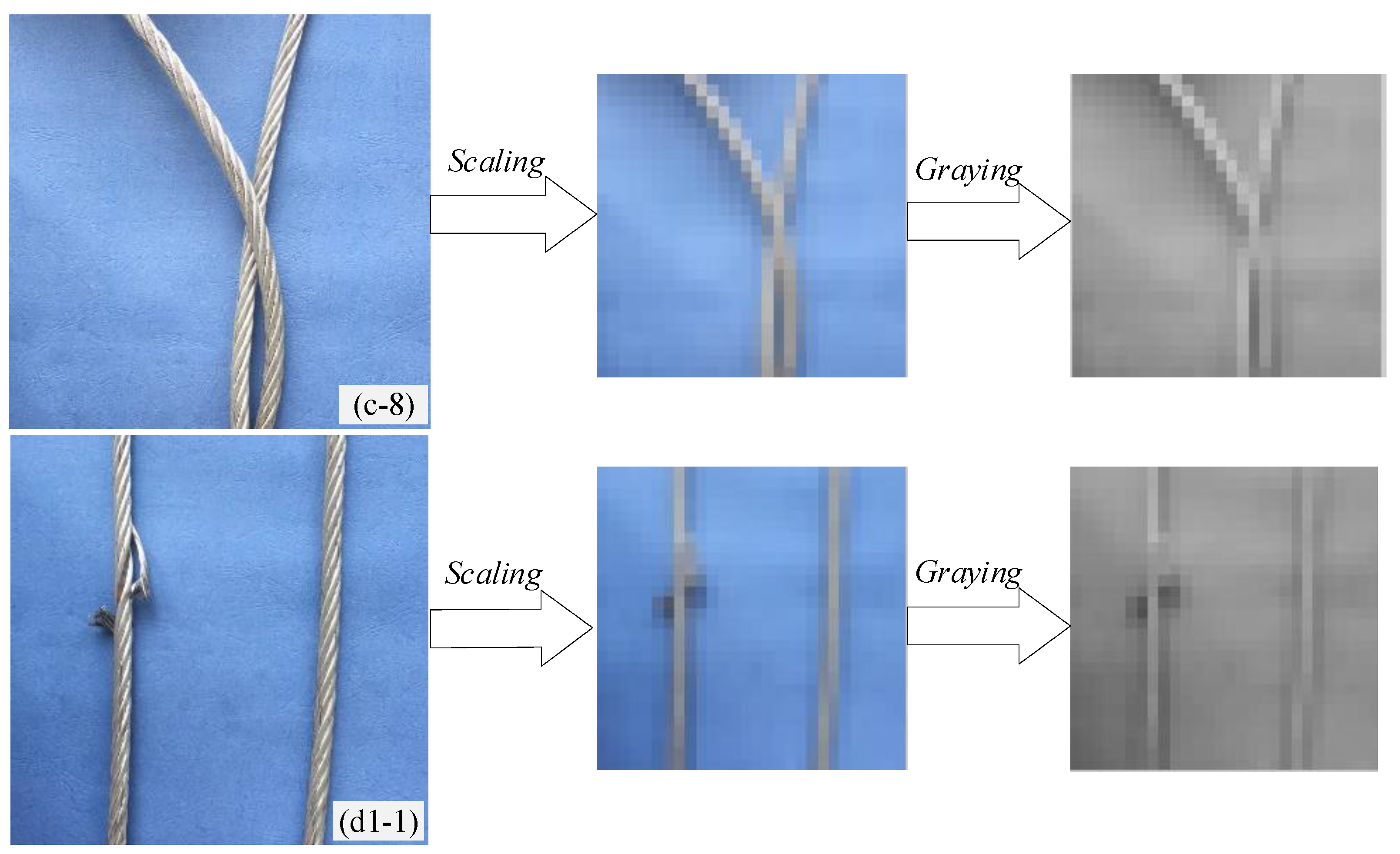
It is known that the images collected by CCD cameras under actual working conditions are of two wire ropes in different states, with the position of the wire ropes and the state of the broken strand on the ropes being the main image characteristics. The recognition results should not be influenced by the image background, oil pollution on the wire rope surface, obvious light changes, and so on. After image preprocessing, the experimental dataset is essentially consistent with the actual scene dataset, which is a 28 × 28 gray pixel matrix that can directly reflect the position of the wire rope and the shape of the broken strand. In order to further illustrate the feature information of the position and defect of the tail rope after scaling and grayscale processing, we display bilinear interpolation scale images and grayscale images in Figure 7. We randomly selected some images in Figure 6 (e.g., the eighth image of the twisted rope (c-8) and the first image of the broken strand of the left rope (d1-1)), then we used the following image processing method: first, the bilinear interpolation method was used to scale the size to 28 × 28. Then, graying was done. The information of the position and defect features of the tail ropes are clearly visible in the scaling and graying images. Because the CNN is not sensitive to the scale and rotation of the input image data, it can automatically mine and learn the potential feature information of the dataset.

The nine kinds of tail rope states are given in

Table 3. The nine kinds of tail rope states.

Tail Rope States	CNN Sample Number	Label	One Hot Coding
Normal (NM)	500	1	100000000
Disproportional spacing (DS)	500	2	010000000
Twisted rope (TR)	500	3	001000000
Broken strand of the left rope (BS-LR)	500	4	000100000
Broken strand of the right rope (BS-RR)	500	5	000010000
Broken strand of double ropes (BS-DR)	500	6	000001000
Left broken rope (L-BR)	500	7	000000100
Right broken rope (R-BR)	500	8	000000010
Double broken ropes (D-BR)	500	9	000000001

.

5. Experiment and Analysis

This section describes our experiment and presents the analysis of the obtained results. Firstly, we propose the evaluation methodology and metrics for the performance measure. Secondly, we describe the data mining of the tail rope dataset using the CNN. Then, we provide a comparison with other traditional intelligent methods (e.g., KNN and ANN-BP) that we used to carry out the BTR fault diagnosis. Finally, the results of each algorithm are compared and analyzed. During the study of the different algorithms, the related parameters are adjusted to achieve better accuracy, the hold-out method is used to verify its generalization performance, and the diagnosis results are analyzed using the confusion matrix.

5.1. Evaluation Methodology and Performance Measure

In general, in the actual task, we need to evaluate the generalization error of the model, and then choose the model with the smallest generalization error. Therefore, it is necessary to use the testing set to test the discriminant ability of the model, and then take the test error of the testing set as an approximation of the generalization error. The testing set and training set are usually mutually exclusive, (i.e., the test samples do not appear in the training set and are not used in the training process). Therefore, this paper uses the hold-out method [40] to evaluate the model. The hold-out method directly divides the data set D into two mutually exclusive sets, namely the training set A and the testing set B (D = A$\cup$B, A$\cap$B = Ø) [41]. After the model is trained using training set A, testing set B is used to evaluate the test error as an estimate of the generalization error.

After evaluating the generalization performance of the model, it is necessary to measure the performance of the model with evaluation metrics. In this paper, four evaluation metrics are calculated, namely accuracy, precision, recall and f1-score. Their formulas can be seen in Equations (9)–(12) [22]:

$$\mathrm{a}ccuracy=\frac{TP+TN}{TP+FP+FN+TN},$$

(9)

$$precision=\frac{TP}{TP+FP},$$

(10)

$$recall=\frac{TP}{TP+FN},$$

(11)

$$f1-score==2\frac{precision\times recall}{precision+recall},$$

(12)

where TP means true positive, FP means false positive, TN represents true negative, and FN represents false negative. All of them are classified according to the combination of the real category and model prediction category [42]. Taking the binary classification as an example, the confusion matrix of the classification results is shown in

Table 4. The confusion matrix of the binary classification results.

Real Situation	Predicted Results
	Positive	Negative
Positive	TP	FN
Negative	FP	TN

. It is clear that the total number of samples equals the result of the formula TP + FP + TN + FN.

Different metrics directly reflect the impact of health monitoring tasks. For example, accuracy can directly reflect the number of correct and erroneous prediction results for all of the test samples. Precision can reflect a certain category of test samples, how many predictions are correct, and how many predictions are incorrect. For example, if in a testing set containing 100 samples of twisted rope, 90 are predicted to be twisted rope faults and 10 are classified as other faults, the precision for the twisted rope fault is 90%. Recall and precision are a pair of contradictory measurements. Recall shows how many predictions are correct in a certain class of prediction results. For example, if 100 prediction results are twisted rope faults, of which 90 test samples are actually twisted rope faults and 10 test samples are other faults, then the recall of the twisted rope fault is 90%. A good classifier maximizes both precision and recall to make fewer incorrect prediction results, which is expressed in the f1-score. The f1-score is the harmonic average of precision and recall.

The tail rope health monitoring in this paper is a multi-classification task. According to Section 4, different kinds of features, including normal (a), disproportional spacing (b), twisted rope (c), broken strand (d), and broken rope (e), should not normally be predicted incorrectly because their features are quite different. It may be difficult for classifiers to classify similar categories, for example, classifying between subcategories of broken strand (d): broken strand of the left rope (d1), broken strand of the right rope (d2), and broken strand of double ropes (d3). If the defects on the left or right were to change in size, shape, or height, it is possible that broken strand of double ropes (d3) would be predicted as broken strand of the left rope (d1) or broken strand of the right rope (d2), or vice versa. In addition, for the faults left broken rope (e1), right broken rope (e2), and double broken ropes (e3) in the category broken rope (e), when the position or height of the broken rope change, it is easy to predict double broken ropes (e3) as left broken rope (e1) or right broken rope (e2), or vice versa.

In the following, the performance of the classifiers is measured with the metrics given by Equations (9)–(12), and the prediction results are visualized by the confusion matrix.

5.2. Computation and Results Analysis

5.2.1. The Convolutional Neural Network

(1) CNN parameters selection

Concerning the CNN configuration, it is still an open question what hyper-parameters (e.g., number of layers, learning rate, size of the filters, batch-size, etc.) are useful to a greater or lesser extent for this task [42]. The hyper-parameters are adjusted in order to study the performance of the built CNN. 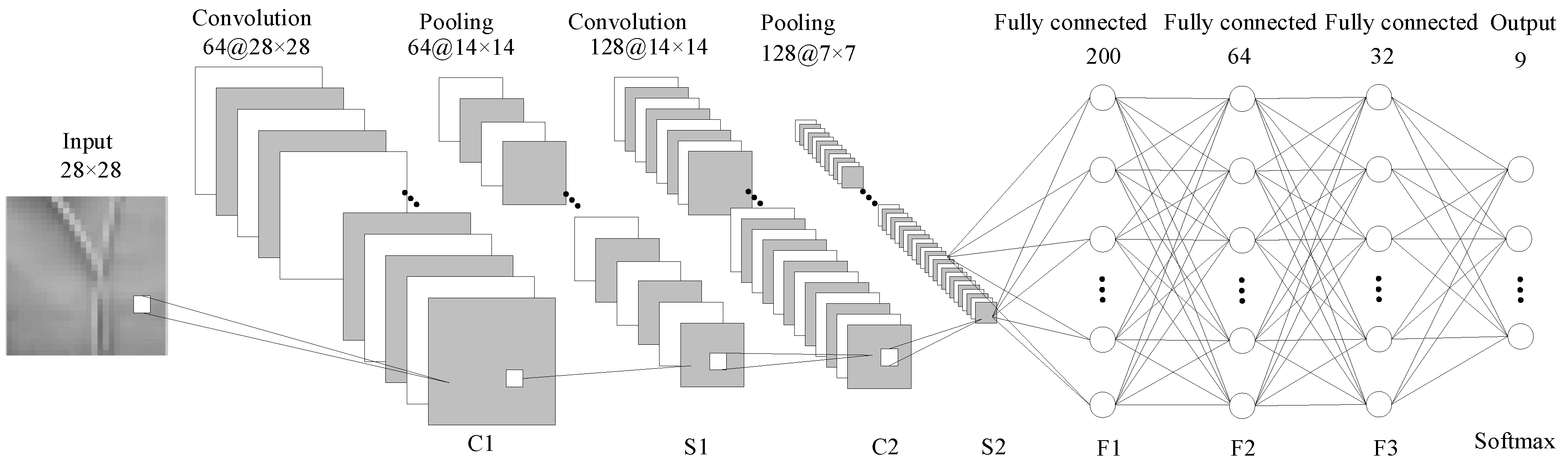The choice of learning rate and batch-size severely affects the training and testing results, so we adjust and study the learning rate and batch-size in this paper [20]. The structure of CNN is shown in Figure 3, and the configurations of each layer are listed in Table 1. In addition, before each round of training, the dataset is randomly disturbed, the network parameters are randomly initialized, the L₂ regularization term is added to the fully connected layer F1, and a stochastic gradient descent (SGD) algorithm is used to train the network [35]. Before the training and testing of the BTRs dataset, 70% of the total sample is selected randomly as the training sample, and the remaining 30% is used as the testing sample (i.e., 3150 samples are selected as the training dataset and 1350 samples are used as the testing dataset). After training and testing, we mainly use Equation (9) (accuracy) to evaluate the performance of the CNN.

(a) Learning rate

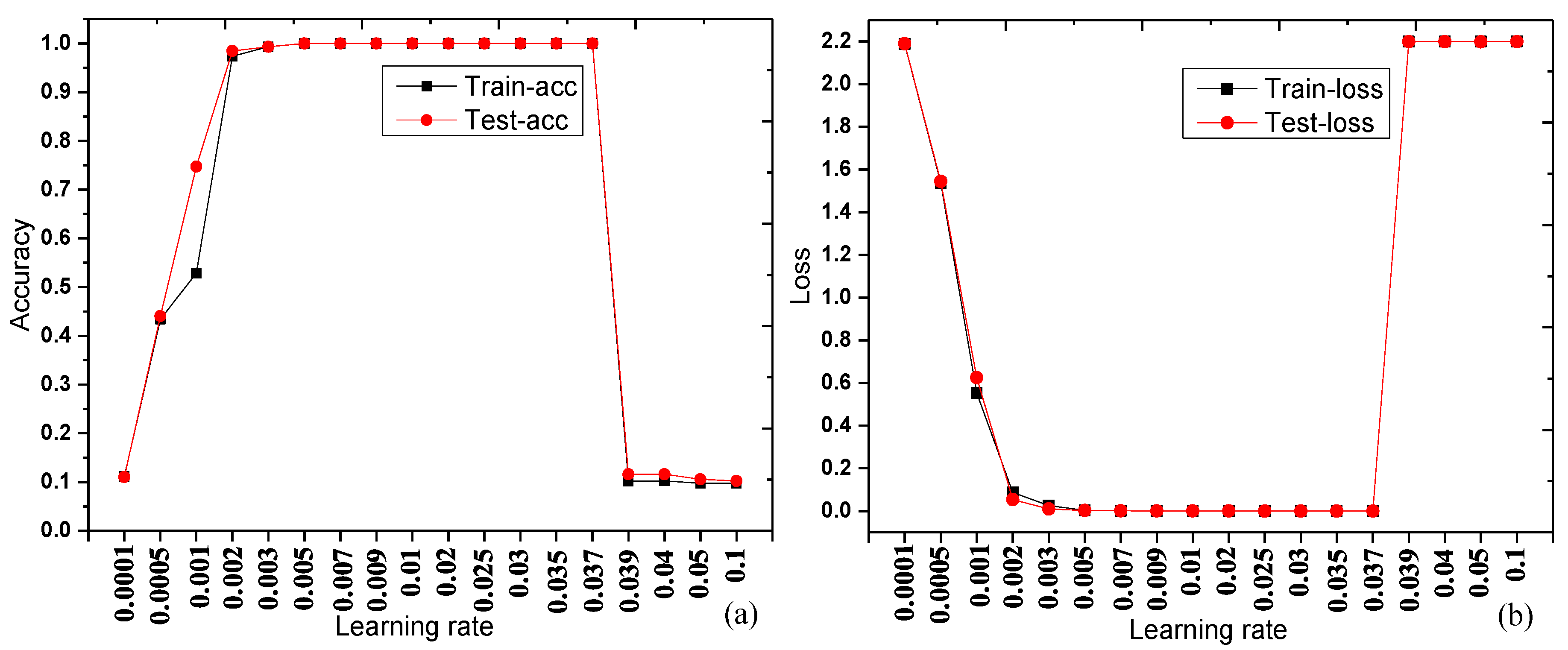
An ideal learning rate will accelerate the convergence of the model, while an undesirable learning rate will even directly cause the loss of the objective function to explode and fail to complete the training [43]. In this section, the network iteration is set to 40 epochs, and the initial batch-size is set to 5. The training loss, training accuracy, testing loss and testing accuracy under different learning rates are shown in

Table 5. The loss and accuracy (Acc) under different learning rates.

Learning Rate	Train-Loss	Train-Acc	Test-Loss	Test-Acc
0.0001	2.1880	0.1114	2.1890	0.1104
0.0005	1.5374	0.4343	1.5445	0.4407
0.001	0.5529	0.5286	0.6247	0.7474
0.002	0.0870	0.9737	0.0535	0.9844
0.003	0.0257	0.9933	0.0095	0.9932
0.005	0.0030	1	0.0028	1
0.007	0.00086	1	0.00086	1
0.009	0.00041	1	0.00045	1
0.01	0.00033	1	0.00037	1
0.02	0.000085	1	0.000094	1
0.025	0.000048	1	0.000054	1
0.03	0.000051	1	0.000056	1
0.035	0.000033	1	0.000035	1
0.037	0.000033	1	0.000036	1
0.039	2.1990	0.1016	2.1989	0.1163
0.04	2.1991	0.1022	2.1990	0.1163
0.05	2.1990	0.0978	2.1981	0.1056
0.1	2.2005	0.0978	2.1990	0.1022

.

From the data in Table 5, the training and testing curves are made as shown in Figure 8. Table 5 and Figure 8 show that both the training accuracy and testing accuracy are 100% around the learning rate of 0.01, and that the accuracy is highest and stable at this rate. During training and testing, the accuracy and loss of testing are basically consistent with the training accuracy and loss, indicating that there is no significant noise in the dataset, and the network performance is good. With the increase in the learning rate, the training accuracy and the test accuracy first increase, then remain stable, and finally reduce quickly (training loss and testing loss decrease at first, then keep stable, finally increase and keep stable), indicating that smaller and larger learning rates reduce the accuracy of the network. Therefore, in this experiment, the optimized learning rate is set to 0.01.

(b) Batch-size

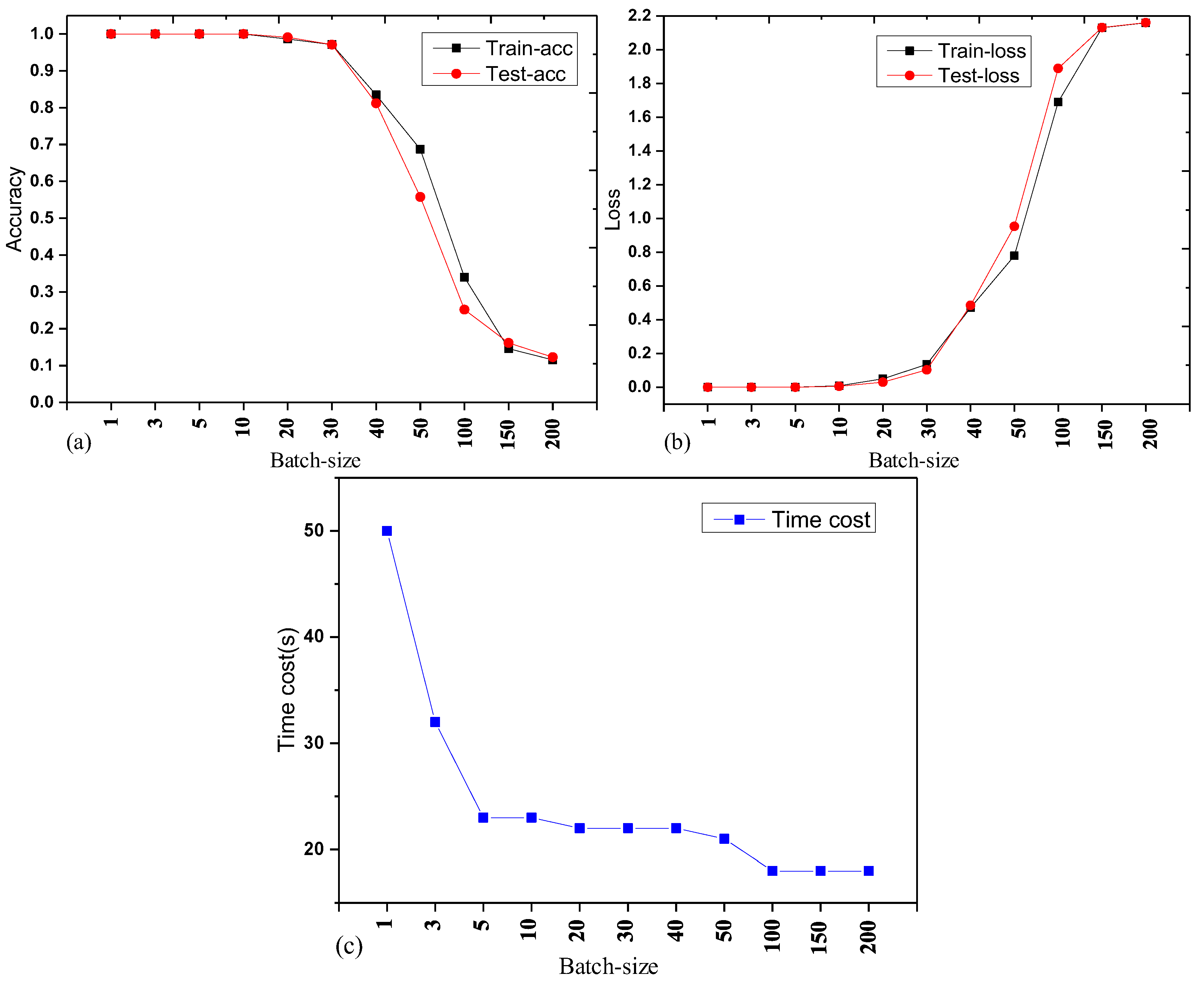
When the SGD method is adopted, the batch-size has a great influence on network performance. In this section, we set the network iteration to 40 epochs, and the learning rate to 0.01. The training loss, training accuracy, testing loss, testing accuracy, and time cost of different batch-sizes are shown in

Table 6. The loss, accuracy, and time cost under different batch-sizes.

Batch-Size	Train-Loss	Train-Acc	Test-Loss	Test-Acc	Time Cost (s/epoch)
1	0.000021	1	0.000019	1	50
3	0.00012	1	0.00014	1	32
5	0.00033	1	0.00037	1	23
10	0.0084	0.9997	0.0052	1	23
20	0.0500	0.9860	0.0299	0.9911	22
30	0.1350	0.9711	0.1030	0.9711	22
40	0.4711	0.8346	0.4853	0.8119	22
50	0.7783	0.6870	0.9526	0.5578	21
100	1.6900	0.3394	1.8885	0.2519	18
150	2.1296	0.1460	2.1309	0.1615	18
200	2.1587	0.1156	2.1601	0.1230	18

.

The training and testing curves are made as shown in Figure 9, according to the data in Table 6. From Table 6 and Figure 9, it is known that when the batch-sizes are 1, 3, and 5, the training accuracy and testing accuracy are both 100%, and that the accuracy is the highest and stable. With the increase in the batch-size, the training accuracy and testing accuracy remain stable at first, then reduce quickly (training loss and testing loss keep stable at first, then increase fast), indicating that larger batch-sizes reduce the accuracy of the network. It is also found that larger batch-sizes led to less time being consumed for each iteration. If we use graphics processing units (GPUs) to accelerate the computation process via parallel computation, we can significantly reduce the iteration time. Therefore, in this experiment, when the learning rate of the CNN model is set to 0.01 and the batch-size is set to 5, the training and testing accuracies are high, and the time consumption of each iteration is less, meeting the requirements of accuracy and real time.

(2) Detailed Results

(a) Hold-out method

The hold-out method [40] is used to evaluate the generalization error of the model. First, 4500 samples are randomly disturbed and then a certain proportion of these samples are chosen for training and testing using the hold-out method. Each training lasts for 40 epochs and the evaluation metrics of the test data set are calculated according to Equations (9)–(12). After training and testing five times and calculating the mean value, the results are shown in

Table 7. The different dividing ways of the hold-out method.

Dividing Ways (Train (%)-Test (%))	Train-Loss	Test-Loss	Accuracy	Precision	Recall	f1-Score	Approximate Time Cost (s/epoch)
60–40	0.00049	0.00047	1	1	1	1	21
65–35	0.00064	0.00065	1	1	1	1	26
70–30	0.00033	0.00037	1	1	1	1	27
75–25	0.00037	0.00039	1	1	1	1	32
80–20	0.00024	0.00026	1	1	1	1	35

.

According to Table 7, we find that the method of dividing the dataset between training and testing has little effect on the experimental results, and that the four metrics under each division are all 1, with only a small difference in the loss and time consumption. These results demonstrate that the established CNN network model has a good performance.

In similar applications of machine learning and CNNs for image classification, approximately 2/3~4/5 samples are generally used for training and the rest are used for testing [44]. Therefore, we use 75% of the data for training and 25% of the data for testing in the next part.

(b) Iterative process

Through all of the above studies, we adopt the CNN structure proposed in Section 3, combined with the Table 1, to determine the following network settings:

• The dataset is randomly divided using the hold-out method, 75% is divided into the testing set, and 25% is divided into the training set;
• The learning rate is set to 0.01, the batch size is set to 5, and the iteration is set to 40;
• The fully connected layer F1 is processed using L₂ regularization;
• The network is trained using an SGD algorithm.
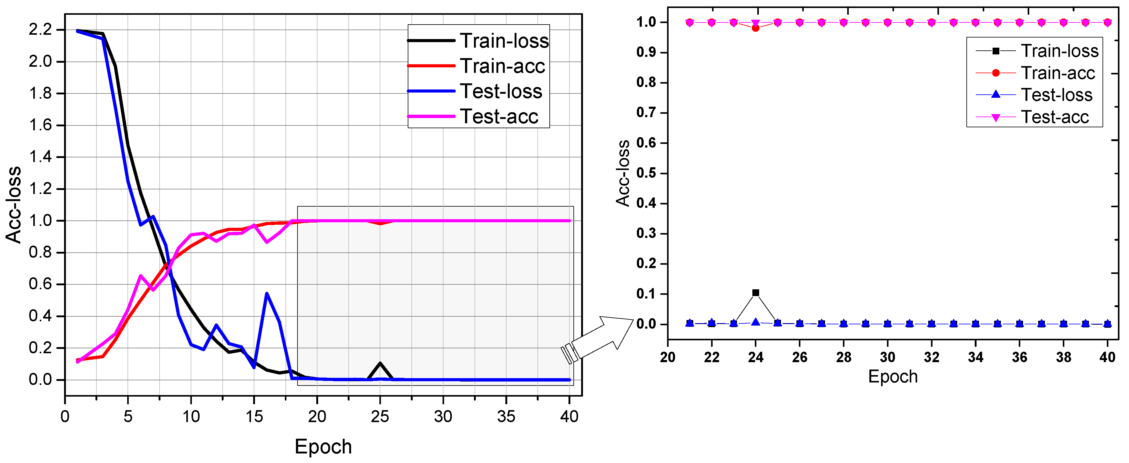
• The iterative process of training and testing for 40 epochs is shown in Figure 10.

From Figure 10, it can be seen that during the 40-epoch iterative process: the training accuracy and testing accuracy increase rapidly and approach 100%, reaching 90% in approximately 10 rounds, and reaching 99% in around 17 rounds. The training loss and testing loss converge quickly and eventually close to 0.0002. The training accuracy is consistent with the testing accuracy in the iterative process, as well as the training loss and testing loss. The testing results are as good as the training results, which shows that due to the regularization processing of the network, there is no overfitting phenomenon and the generalization performance is good. After 20 rounds, the training and test curves are relatively smooth, indicating that there is no need to iterate for 40 rounds to achieve a better effect. Meanwhile, the time consumption of each iteration is less (32 s/epoch, 10 ms/step).

(c) Confusion matrix

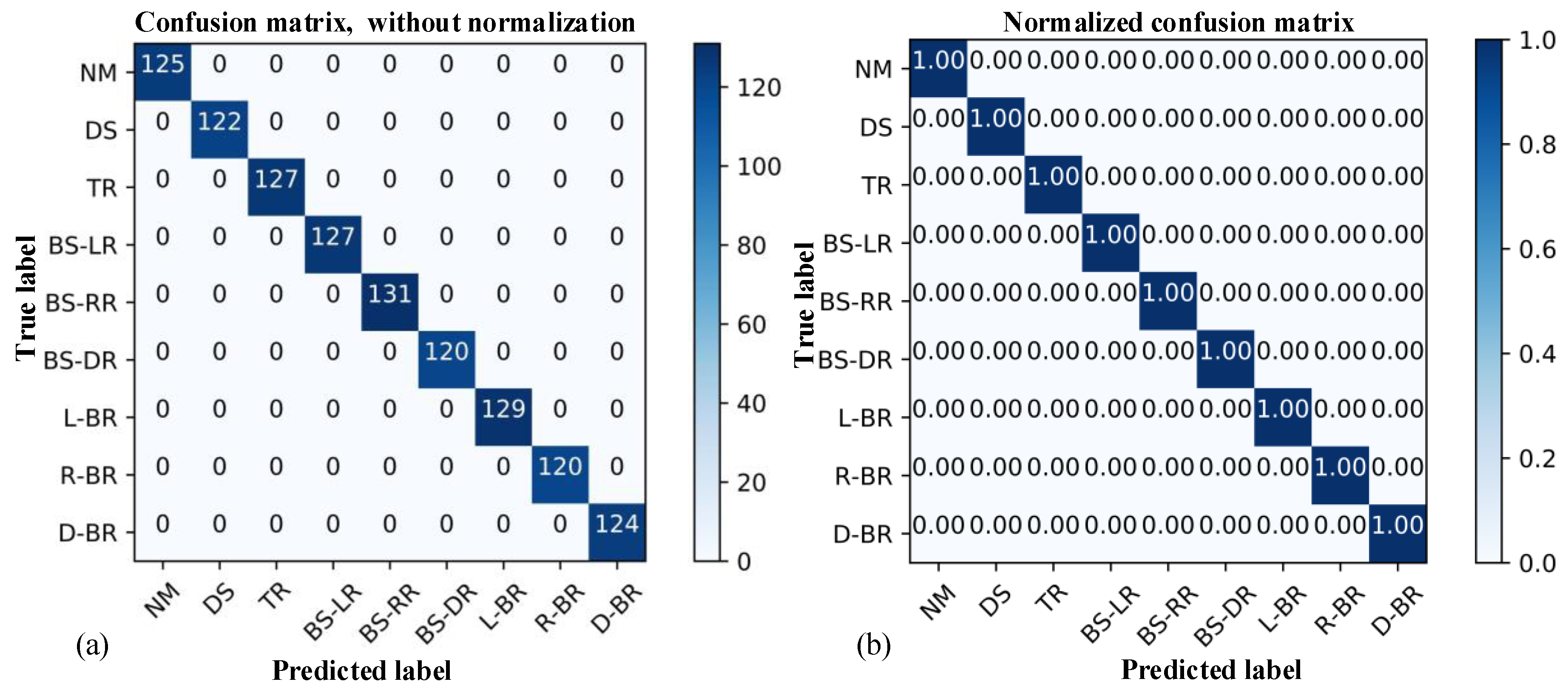
A confusion matrix is used to present the performance and the result of the CNN, as shown in

Table 8. The confusion matrix of the CNN.

Matrix	Precision	Recall	f1-Score	Support
NM	1	1	1	125
DS	1	1	1	122
TR	1	1	1	127
BS-LR	1	1	1	127
BS-RR	1	1	1	131
BS-DR	1	1	1	120
L-BR	1	1	1	129
R-BR	1	1	1	120
D-BR	1	1	1	124
Average/total	1	1	1	1125

and Figure 11. The accuracy, precision, recall, and f1-score are all 1 for the 1125 prediction samples, and the prediction results of each category are exactly the same as the actual results (labels), indicating the good performance of the CNN algorithm. The CNN has a good prediction ability for the tail rope faults, can completely separate the nine kinds of tail rope states, and can accurately predict them.

Therefore, the convolutional neural network for the health monitoring and fault diagnosis of hoisting system BTRs proposed in this paper presented a good performance, meeting the requirements of accuracy, real-time functioning, and generalization performance.

5.2.2. The k-Nearest Neighbor and Artificial Neural Network with Back Propagation

(1) KNN

The KNN [45] is a classification method based on statistics. It was first proposed by Cover and Hart in 1968. As the simplest machine learning method, the algorithm is relatively theoretically mature and is widely used in classification tasks [46]. This algorithm performs the following operations on each unknown category in the dataset:

Step 1. The distance between the point of the dataset with a known class and the current point is calculated;

Step 2. The distances are sorted according to increasing order of distance;

Step 3.k points with the minimum distance are selected from the current point;

Step 4. The occurrence frequency of the category of the previous k points is determined;

Step 5. The class with the highest frequency of the previous k points is selected as the pre-classification of the current point.

In Step 1, computing the distance includes the Euclidean distance, Manhattan distance, etc. (the latter one is utilized in this paper). The eigenspace $\chi$ is an n dimensional real vector space Rⁿ, where $x_i,x_j\in \chi$, $x_i={(x_i{}^{(1)},x_i{}^{(2)},\cdot \cdot \cdot ,x_i{}^{(n)})}^{\mathrm{T}}$, $x_j={(x_j{}^{(1)},x_j{}^{(2)},\cdot \cdot \cdot ,x_j{}^{(n)})}^{\mathrm{T}}$. The Manhattan distance of $x_i,x_j$ is:

$$L_1(x_i,x_j)={\displaystyle \sum _{l=1}^n\left|x_i^{(l)}-x_j^{(l)}\right|}$$

(13)

In practical applications, the choice of the k value should not be too small or too large, because the prediction results are very sensitive to the value of k [47]. For example, we choose a few k values, such as 7, 10, 13, 15, and 20, and the accuracy results are 85.24%, 88.44%, 86.67%, 85.42%, and 81.33%, respectively, which illustrates that the accuracy of each prediction with different k values is quite different. To find the k nearest neighbor points quickly, we use the ball-tree [48]. 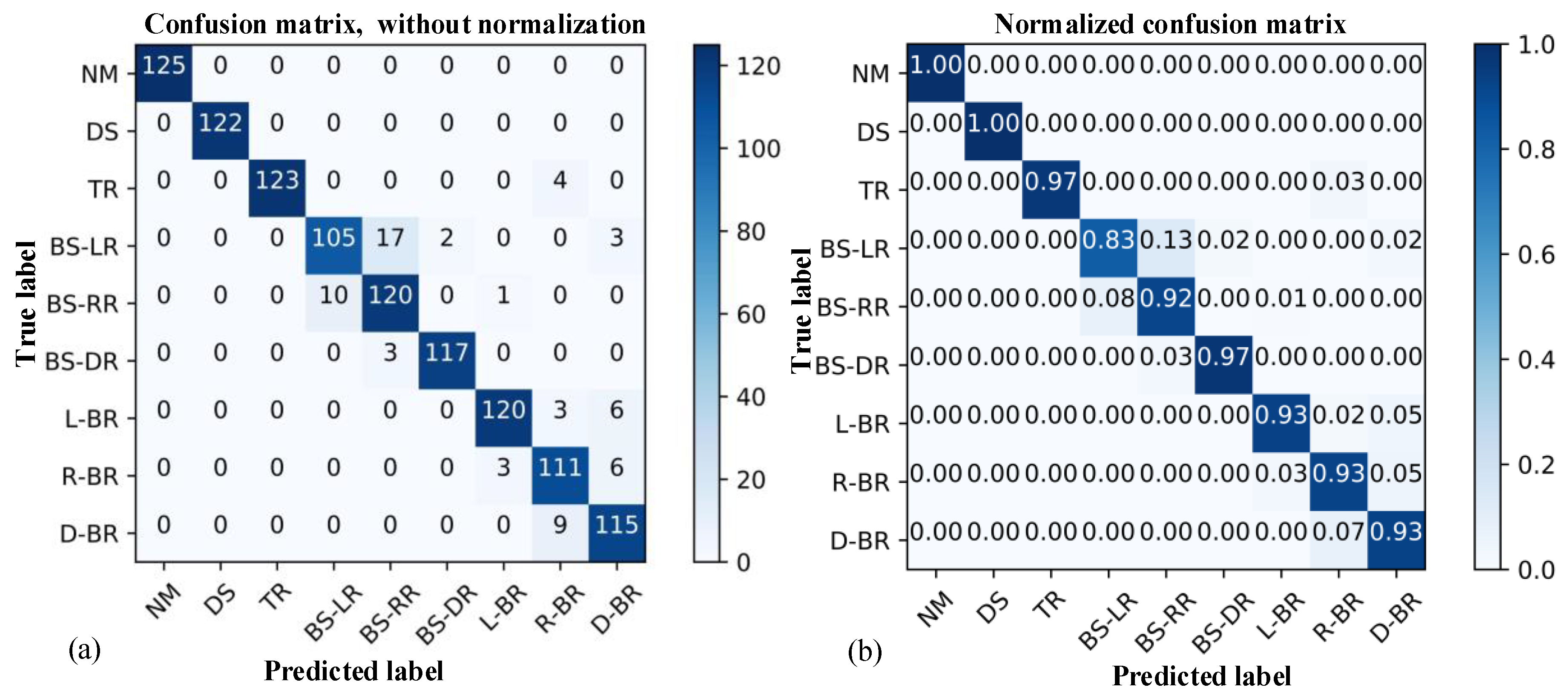The ball-tree is suitable for high-dimensional problems, generally when the feature dimension is greater than 20 [49]. In this paper, the dimension of the dataset is 784. After adopting the ball-tree in KNN, the prediction accuracy is 94.04% and the time consumption is 50 s. The confusion matrix of the prediction result is shown in Figure 12.

As depicted in Figure 12, the precision of the normal (NM) and disproportional spacing (DS) states is 1, which is the highest. The precision of the broken strand of the left rope (BS-LR) is 0.83, which is the lowest yielded result. The prediction results show that the main prediction errors occur among similar fault types. For example, for the 127 BS-LR faults, 17 are predicted as the broken strand of the right rope (BS-RR) type; for 131 BS-RR faults, 10 are predicted as the BS-LR type; and for 124 double broken rope (D-BR) faults, 9 are predicted as the right broken rope (R-BR) type. The results demonstrate that KNN has some shortcomings in distinguishing similar fault types (consistent with the hypothesis analysis in Section 5.1), and the accuracy is lower than that of the CNN algorithm.

(2) ANN-BP

The ANN-BP is a typical model that uses an error back-propagation algorithm to train the weights and biases of each neuron, and it contains several layers (i.e., input layer, output layer, and hidden layers) [50]. The ANN-BP has a relatively simple structure, and thus it has been widely used in fitting nonlinear continuous functions and pattern recognition [51].

The training and testing processes are shown in Figure 13 using the same structure as the CNN’s fully connected layer (784–200–64–32–9) and the same network settings proposed in this paper (i.e., using the hold-out method; the learning rate is set to 0.01; the batch size is set to 5; the iteration is set to 40 epochs; the SGD algorithm is used, etc.). According to Figure 13, the testing accuracy is 96.44%, lower than the diagnostic accuracy of the CNN, showing the importance of the convolutional operation of CNN in feature extraction. Compared with Figure 10, it can be seen that the iterative process of the designed CNN model is more stable than that of the ANN-BP.

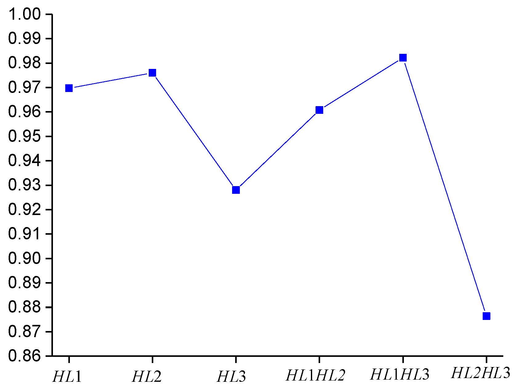
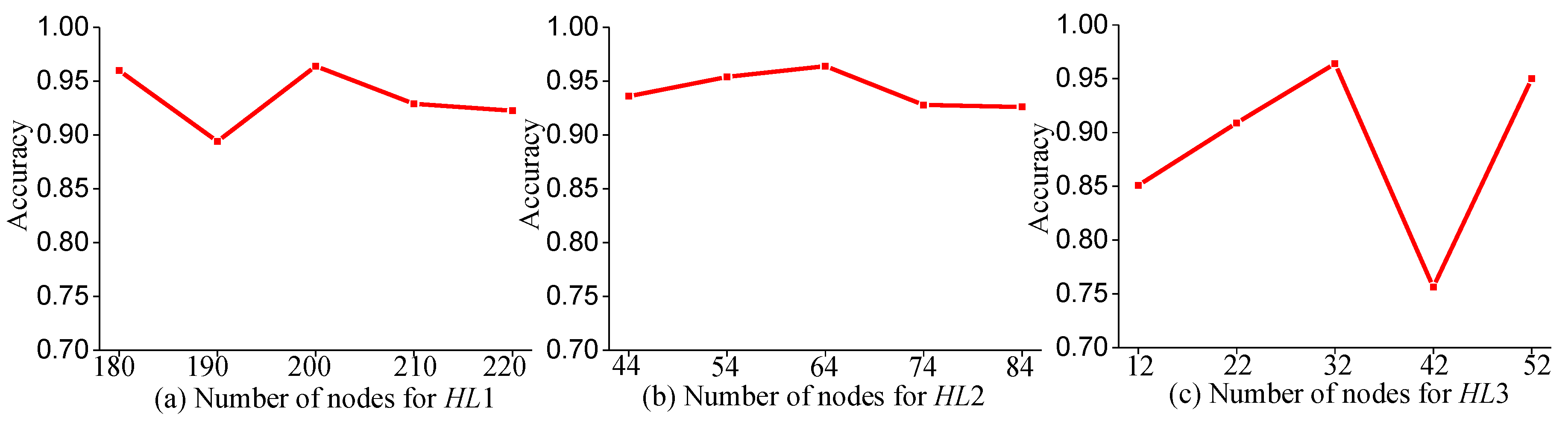
To study the influence of the number of hidden layers and the number of nodes per layer on the performance of ANN-BP, we attempt to fine-tune the structure of the network in order to study its prediction performance. The three hidden layers of ANN-BP are denoted as HL1, HL2, and HL3, respectively. Firstly, the number of hidden layers is changed, including HL1, HL2, HL3, HL1HL2, HL2HL3, and HL1HL3, and the prediction accuracy results are shown in Figure 14. Then, the number of nodes in each layer is changed, (i.e., HL1 is varied from 180 to 220, HL2 from 44 to 84, and HL3 from 12 to 52), and the prediction accuracy results are shown in Figure 15.

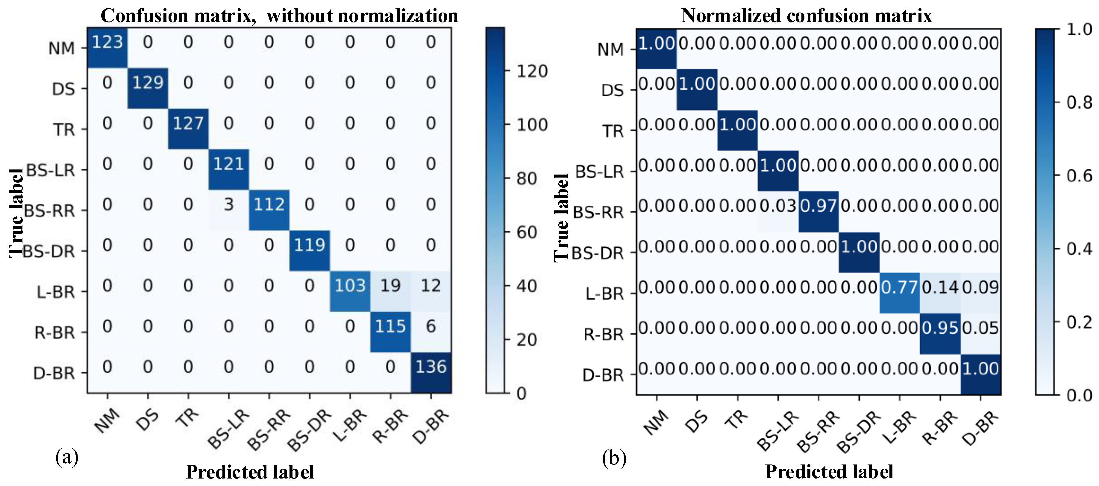
Through analysis, we find that ANN-BP is sensitive to the number of network layers and the number of nodes in each layer, and the prediction accuracy does not reach 100%, meaning that the prediction accuracy of ANN-BP is less than that of the CNN proposed in this paper. To visualize the prediction results, we display the confusion matrix of ANN-BP in Figure 16. According to Figure 16, the precision of NM, DS, twisted rope (TR), BS-LR, BS-DR, and D-BR is 1, which is the highest. The precision of the left broken rope (L-BR) is 0.77, which is the lowest value attained. The prediction results show that the main prediction errors occur among similar fault types. For example, among the 134 L-BR faults, 19 are predicted as the R-BR type and 12 are predicted as the D-BR type; among the 121 R-BR fault types, 6 are predicted as the D-BR type. The results show that ANN-BP and KNN have some deficiencies in distinguishing similar fault types, which is consistent with the hypothesis analysis in Section 5.1.

5.2.3. Comparative Analysis of Results

The results of the different algorithms evaluated in this paper are listed in

Table 9. The different algorithm results.

Algorithm	Description	Accuracy	Time Cost
KNN	Using ball-tree structure	94.04%	50 s
ANN-BP	Structure is 784–200–64–32–9	96.40%	1 s/epoch, 385 µs/step
Proposed CNN	Structure is Input (28 × 28)–64C(3 × 3)–64P(2 × 2)–128C(3 × 3)–128P(2 × 2)–FC(200–64–32)–Output(9)	100%	32 s/epoch, 10 ms/step

. In summary, through the training and testing of the BTR dataset, the CNN model achieved a diagnostic accuracy of 100% (it could accurately identify and predict all tail rope statuses), which was higher than the 94.04% of KNN and the 96.44% of ANN-BP. The time consumption of each iteration was 32 s, with each step being 10 ms, which meets the requirements of system accuracy and real-time functioning. Additionally, the L₂ regularization process of the fully connected layer F1 could prevent overfitting, which allowed the network to achieve a good generalization performance. Although ANN-BP had less time consumption, its accuracy and stability were worse than those of CNN. At the same time, KNN was worse than CNN in terms of accuracy and time consumption. Therefore, we can clearly conclude that the performance of CNN was better than that of KNN and ANN-BP for the health monitoring of tail ropes. Therefore, the CNN model is more suitable for the actual health monitoring of hoisting systems.

6. Industrial Application Plan

This paper describes a method for the health monitoring and fault diagnosis of balancing tail ropes. The object of this research was a hoisting system with two balancing tail ropes, but the same approach used in this paper can be used to construct a dataset for hoisting systems with three or more tail ropes. The industrial application plan is: first, configure the related hardware and software shown in Figure 1, and conduct explosion protection for the related devices; after the system is debugged, a large number of tail rope images are collected at the scene and the image dataset of the actual working conditions is set up; then, these data are used as the input to train the CNN or fine-tune the trained CNN. Deep learning can also be introduced into the safety monitoring of the whole hoisting system in order to realize the data mining and fault diagnosis for other key components (e.g., the drive motor, reducer, brake system, hoisting wire rope, etc.), expanding the system’s applicability beyond just the tail ropes.

In our experimental environment, it took less than 10 ms to complete the prediction of one sample, and the prediction accuracy was 100%. The use of a graphics processing unit will reduce the time cost. A larger dataset will improve the generalization performance of the network, and the network prediction accuracy will also be higher and stable. Therefore, the CNN can be used in industrial applications.

7. Conclusions and Future Work

Aiming at the problems of high difficulty, high risk, and low recognition efficiency in the existing artificial detection methods for fault detection in BTRs, a health monitoring method for the balancing tail ropes of a hoisting system based on a convolutional neural network is proposed in this paper. In this method, the real-time tail rope images are first captured through CCD cameras and the data transmission is realized using a movable sensor network in the vertical shaft. Then, the preprocessed images are input to train the convolutional neural network in order to realize the automatic recognition of the BTR faults. Finally, fault warnings are made based on the identification results. The research can be summarized and concluded as follows:

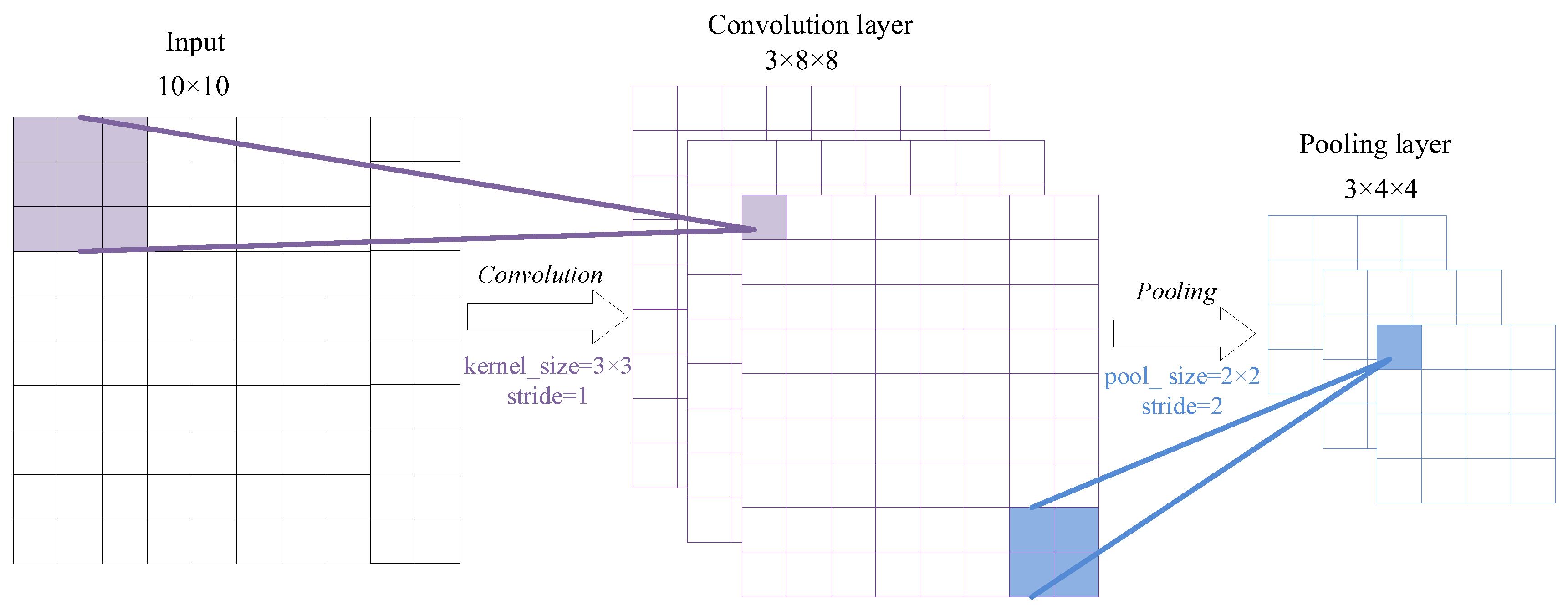
(1) A CNN including two convolution layers, two pooling layers, and three fully connected layers is proposed. The structure of the CNN is denoted as Input(28 × 28)–64C(3 × 3)–64P(2 × 2)–128C(3 × 3)–128P(2 × 2)–FC(200–64–32)–Output(9), meaning that the dimensions of the input 2D data are 28 × 28; the CNN first applies 1 convolutional layer with 64 filters and the filter size is 3 × 3. Then, one maximum-pooling layer with pooling size 2 × 2 is used. One convolutional layer with 128 filters (filter size is 3 × 3) is applied next, after which one pooling layer whose pooling size is 2 × 2 is applied. Finally, three fully connected layers whose hidden neuron numbers are 200, 64, and 32, respectively, are applied. The size of the output layer is 9, which is equal to the number of fault types.

(2) A method for the description and establishment of an image dataset that can cover the entire feature space of overhanging BTRs is proposed. The BTRs image dataset covering the 9 features in the state space is set up and further expanded to a scale of 4500 by scale and rotation to enhance the generalization ability of the network model. The same method can be used to describe data from hoisting systems containing more than two tail ropes.

(3) The CNN, KNN, and ANN-BP algorithms were used to train and test the established tail rope image dataset, and the effects of the hyper-parameters of the network diagnostic accuracies were investigated experimentally. The experimental results showed that the feature of the BTR image was adaptively extracted by the CNN’s convolutional and pooling operations, which means that a great deal of manpower can be saved and online updates can be realized, so as to meet real-time requirements. The learning rate and batch size seriously affected the accuracy and training efficiency, with the better values of the learning rate and batch size being 0.01 and 5, respectively. The L₂ regularization process of the fully connected layer F1 could prevent overfitting. The fault diagnosis accuracy of CNN was 100%, while that of KNN was 94.04% and that of ANN-BP was 96.40%, so the diagnosis accuracy of CNN was much higher than that of the KNN and ANN-BP algorithms. Additionally, CNN could accurately identify and predict all kinds of BTR states, while ANN-BP and KNN had some deficiencies in distinguishing similar fault types.

Therefore, the CNN had high accuracy, real-time functioning, and a good generalization performance, which are more suitable for application in the health monitoring of hoisting system BTRs. For industrial applications, future work will be to build the monitoring system’s software and hardware architecture. Meanwhile, although the method proposed in this paper obtained a good performance, it also has shortcomings (i.e., if two or more fault features appear in a feature map, it may influence the recognition result). Therefore, in order to solve the problem of multi-fault coupling, the target detection of a BTR feature map based on R-CNN (regions with CNN features) will be the next research direction.