Multi-View Object Detection Based on Deep Learning

Abstract

A multi-view object detection approach based on deep learning is proposed in this paper. Classical object detection methods based on regression models are introduced, and the reasons for their weak ability to detect small objects are analyzed. To improve the performance of these methods, a multi-view object detection approach is proposed, and the model structure and working principles of this approach are explained. Additionally, the object retrieval ability and object detection accuracy of both the multi-view methods and the corresponding classical methods are evaluated and compared based on a test on a small object dataset. The experimental results show that in terms of object retrieval capability, Multi-view YOLO (You Only Look Once: Unified, Real-Time Object Detection), Multi-view YOLOv2 (based on an updated version of YOLO), and Multi-view SSD (Single Shot Multibox Detector) achieve AF (average F-measure) scores that are higher than those of their classical counterparts by 0.177, 0.06, and 0.169, respectively. Moreover, in terms of the detection accuracy, when difficult objects are not included, the mAP (mean average precision) scores of the multi-view methods are higher than those of the classical methods by 14.3%, 7.4%, and 13.1%, respectively. Thus, the validity of the approach proposed in this paper has been verified. In addition, compared with state-of-the-art methods based on region proposals, multi-view detection methods are faster while achieving mAPs that are approximately the same in small object detection.

1. Introduction

Object detection represents a significant focus of research in the field of computer vision [1] that can be applied in driverless cars, robotics, video surveillance and pedestrian detection [2,3,4]. Traditional object detection methods are primarily based on establishing mathematical models according to prior knowledge; such methods include the Hough transform method [5], the frame-difference method [6], the background subtraction method [7], the optical flow method [8], the sliding window model method [9] and the deformable part model method [10]. Specifically, the first four of these methods all operate in a mode based on feature extraction and mathematical modeling, which utilizes certain features of the data to build a mathematical model and then obtains the object detection results by solving that model, whereas the latter two methods operate in a mode based on feature extraction and classification modeling, which combines hand-crafted features (such as SIFT, Scale Invariant Feature Transform [11]; HOG, Histogram of Oriented Gradients [12]; and Haar [13] features) with a classifier (such as SVM [14] or AdaBoost [15]) to obtain the object detection results by classifying the features. Recently, deep learning techniques have revolutionized the object detection field by improving object detection accuracy and robustness. Because deep neural networks can automatically learn different features, object detection based on deep learning is characterized by more abundant features and stronger feature representation capabilities than are possible with traditional hand-crafted features [16].

Currently, the models used in object detection methods based on deep learning can be subcategorized into detection models based on region proposals and detection models based on regression. Models for deep-learning-based object detection based on region proposals first extract candidate regions in the detection area in preparation for subsequent feature extraction and classification. Typical examples of such models include the R-CNN (Regions with CNN features) [17], SPP-net (Spatial Pyramid Pooling Networks) [18], Fast R-CNN [19], Faster R-CNN [20] and R-FCN (Region-based Fully Convolutional Networks) [21] models. By contrast, models for deep-learning-based object detection based on regression divide a feature map using certain rules and establish relationships among the predicted bounding boxes, the default bounding boxes and the ground truths for training. Typical examples of models based on regression include YOLO (You Only Look Once) [22] and SSD (Single Shot Multibox Detector) [23]. Compared with methods based on region proposals, regression-based methods usually achieve better real-time performance. Although the accuracy of regression-based method generally is poorer than that of region-proposals method, the accuracy gap between them is not always large. For example, the accuracy of SSD is comparable to that of Faster RCNN on VOC 2007 test dataset [23]. Therefore, if the accuracy and real-time performance are both taken into consideration, regression-based methods will be a good choice. Nevertheless, the detection performances of both YOLO and SSD on small objects are unsatisfactory [24,25]. The reason is that small objects may not even have any information at the very top layers of the deep learning model and rich representations are difficult to learn from their poor-quality appearance and structure. Therefore, small object detection is a challenge in the object detection based on deep learning.

This paper proposes a multi-view object detection approach based on deep learning, with the aim of improving the performance of regression-based deep learning models when detecting small objects. In the proposed multi-view approach, the object detection results for a set of divided views are merged to improve the object detection capability. Experimental results demonstrate that this design can substantially improve the detection capability for small objects, which is of great value for improving deep learning technology for further applications in object detection.

2. Disadvantage of Classical Object Detection Methods Based on Regression

Currently, the classical object detection methods based on regression are YOLO and SSD. YOLO is a single neural network that can perform object region detection and object classification simultaneously. Unlike early object detection methods based on region proposals, YOLO achieves end-to-end object detection without dividing the detection process into several stages. SSD is a single shot multibox detector that integrates the regression approach of YOLO with the anchor mechanism of Faster R-CNN [20]. On the one hand, the regression approach can reduce the computational complexity of a neural network to improve the real-time performance. On the other hand, the anchor mechanism is helpful for extracting features at different scales and different aspect ratios. Moreover, the local feature extraction method of SSD is more reasonable and effective than the general feature extraction method of YOLO with regard to object recognition. Furthermore, because the feature representations corresponding to different scales are different, a multi-scale feature extraction method [26] has been applied in SSD, thereby enhancing the robustness of object detection at different scales.

Because YOLO divides each image into a fixed grid, the number of detected objects will be limited. For example, consider a grid scale of S × S, where S = 7. Because each grid yields 2 predicted bounding boxes, only 98 predicted bounding boxes are observed in a single detection, which means that no more than 98 objects can be detected at one time. Moreover, because one grid cell can produce predictions for only one class, when objects of two or more classes are located in the same grid cell, they cannot simultaneously be identified. For example, if the input image scale is 448 × 448, then no more than two objects can simultaneously be identified in a single 64 × 64 grid cell, and their classes must be the same. In addition, with respect to YOLO, once the input image has passed through twenty-four convolution layers and four pooling layers, little detailed information can be observed in the resulting feature map. Therefore, YOLO has a relatively poor ability to detect dense small objects.

Unlike YOLO, SSD adopts a multi-scale approach, which means that the feature maps that are used to detect different objects are at different scales. Because each feature map is produced from convolution results at the same level, the convolution receptive fields of the different levels must be different in size. In particular, the receptive field of a high-level convolution layer is significantly larger than those of lower layers, and the extracted information corresponding to a high-level feature layer is more abstract. The more abstract the feature extraction information is, the less detailed the information will be; thus, SSD detection is also insensitive to small objects.

The formula for calculating the convolution receptive field is as follows:

$$S_{\mathrm{RF}}(i)=(S_{\mathrm{RF}}(i-1)-1)N_s+S_f$$

(1)

where $S_{\mathrm{RF}}(i)$ is the size of the convolution receptive field of the $i$-th layer, $N_s$ is the step length, and $S_f$ is the size of the filter.

SSD adopts the anchor mechanism, for which the detection results are directly related to the size of the default bounding box produced from the anchors. The ratio of the default bounding box to the input image can be calculated according to the formula given in [23]. Furthermore, the relationship between the default bounding box and the input image can then be used to determine the region mapped to the input image. To measure the detection capability of a feature map, the minimal default bounding box scale is selected to observe the minimal region mapped to the input image in the feature map.

The mapping of the default bounding box coordinates to the original image coordinates on the feature map is as follows:

$$x_{min}=\frac{c_{\mathrm{x}}-\frac{w_{\mathrm{b}}}{2}}{w_{feature}}{w}_{img}=(\frac{i+0.5}{\left|f_k\right|}-\frac{w_k}{2})w_{img}$$

(2)

$$y_{min}=\frac{c_{\mathrm{y}}-\frac{h_{\mathrm{b}}}{2}}{h_{feature}}{h}_{img}=(\frac{j+0.5}{\left|f_k\right|}-\frac{h_k}{2})h_{img}$$

(3)

$$x_{max}=\frac{c_{\mathrm{x}}+\frac{w_{\mathrm{b}}}{2}}{w_{feature}}{w}_{img}=(\frac{i+0.5}{\left|f_k\right|}+\frac{w_k}{2})w_{img}$$

(4)

$$y_{max}=\frac{c_{\mathrm{y}}+\frac{h_{\mathrm{b}}}{2}}{h_{feature}}{h}_{img}=(\frac{j+0.5}{\left|f_k\right|}+\frac{h_k}{2})h_{img}$$

(5)

where $(c_{\mathrm{x}},c_{\mathrm{y}})$ denotes the center coordinates of the default bounding box, $h_{\mathrm{b}}$ is the height of the default bounding box, $w_{\mathrm{b}}$ is the width of the default bounding box, $h_{feature}$ is the height of the feature map, $w_{feature}$ is the width of the feature map, $\left|f_{\mathrm{k}}\right|$ is the size in the $k$-th feature map, $h_{img}$ is the height of the original image, $w_{img}$ is the width of the original image, and $(x_{min},y_{min},x_{max},y_{max})$ denotes the mapping coordinates of the default bounding box, which is centered at $(\frac{i+0.5}{\left|f_k\right|}),(\frac{j+0.5}{\left|f_k\right|})$ and scaled to a height of $h_k$ and a width of $w_k$ in the $k$-th feature map.

If the SSD_300 × 300 model is adopted, such that the size of the input image is 300 × 300, the feature maps of the model are mainly produced from the Conv4_3, Conv7, Conv8_2, Conv9_2, Conv10_2, and Conv11_2 layers. The sizes of the convolution receptive field and the mapping region of the default bounding box on each feature map are shown in

Table 1. Convolution receptive fields and mapping regions of. the default bounding boxes in Single Shot Multibox Detector (SSD)_300 × 300.

Convolution Layer		Feature Layer
Layer	Convolution Receptive Field	Output Scale	Default Boxes Ratio	Mapping Region Scale
Conv4_3	92 × 92	38 × 38	0.1	30 × 30
Conv7	260 × 260	19 × 19	0.2	60 × 60
Conv8_2	292 × 292	10 × 10	0.38	114 × 114
Conv9_2	356 × 356	5 × 5	0.56	168 × 168
Conv10_2	485 × 485	3 × 3	0.74	222 × 222
Conv11_2	612 × 612	1 × 1	0.92	276 × 276

.

Table 1 shows that at the Conv9_2 level, most feature points of the feature layer are produced by utilizing the information of the entire input image, which results in comparatively weak differentiation among different objects. Additionally, the mapping region of the default bounding box is more than half the size of the input image; thus, when several objects are simultaneously located in the same region, they cannot be distinguished. This problem is common in object detection based on regression. In such cases, small objects can be recognized and located only by using the information from the previous feature layers. Therefore, SSD has a weak object detection capability for small object detection.

3. Multi-View Modeling

3.1. Establishment of a Multi-View Model

This section may be divided by subheadings. It should provide a concise and precise description of the experimental results, their interpretation as well as the experimental conclusions that can be drawn.

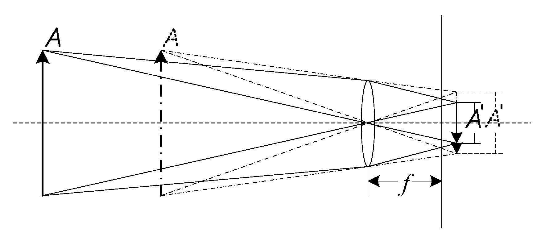
To improve the small object detection performance of a regression-based deep learning model, a region segmentation operation is applied prior to object detection. Each region of the image can be treated as a separate view and magnified to produce more responses on the feature map of the model, in a manner similar to the imaging magnification process observed in the human eye when approaching an object. The details are shown in Figure 1.

In Figure 1, the initial imaging process in the human eye is shown by the solid lines, and $A^{\prime }$ is the real image of object $A$ after imaging. Suppose that the focus of the eye remains unchanged while object $A$ moves a certain distance toward the eye; then, the second imaging process is as shown by the dotted lines. In these two processes, the scale of object $A$ does not change, but the image $A^{\prime }$ appears larger after the second imaging process. More visual nerve cells are triggered to generate a visual response, and the human eye can perceive more information about the object. If the perceived information is insufficient, the human eye will barely be able to recognize the object or may not even see it at all. Similarly, in object detection, objects are recognized and located based on the information contained in the feature map of the detection model. Therefore, increasing the information captured in the feature map is an effective means of improving object detection performance.

To achieve this purpose, a region magnification operation is applied to magnify the RoIs (regions of interest) of the input image. The input image is divided into four equal regions: upper left, upper right, bottom left and bottom right. In additional, because more salient information is usually contained in the central area, a center region is added along with the above four regions. The center region has the same center point as the input image and 1/2 its scale in both the horizontal and vertical directions. Finally, the five regions are interpolated to generate five images of the same size as the original image. Then, when the images are input into the deep learning model, more response will be obtained in the same level feature map. The details of magnification operation are shown in Figure 2.

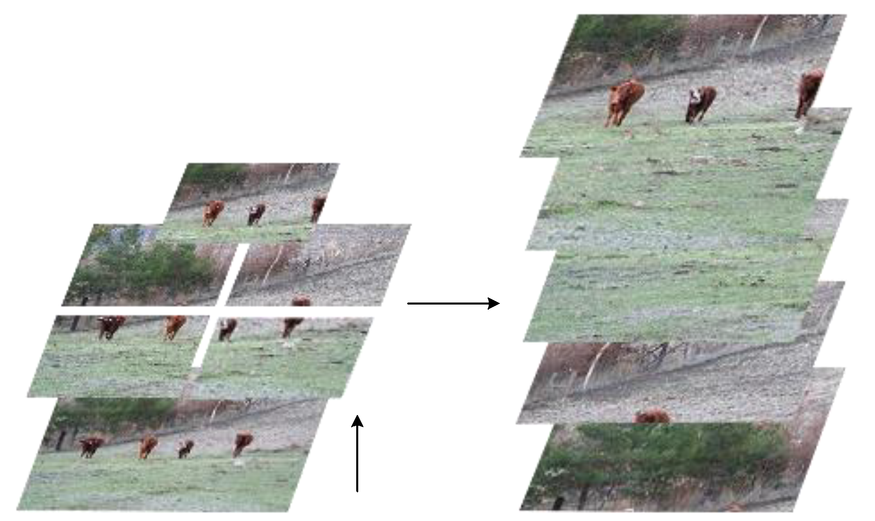
The module that performs the operation described above is called the multi-view module. During the detection process, a set of detection results will be acquired for each region after a single detection; thus, five sets of object detection results will be generated. Because the original image is cut into different regions, a cutting phenomenon will be observed in the detection results. Therefore, a merging module is needed at the end of the process. The merging module integrates the results obtained for each region to yield the final detection results. An overview of the entire detection model is shown in Figure 3.

As shown in Figure 3, when an image is input into the model, it first passes through the multi-view module and is cut into five detection regions. Then, these five detection regions are passed to the detection model (YOLO/SSD) for detection. Finally, the detection results are sent to the merging module, which applies the region splicing and region merging operations to obtain the final detection results. The applicability of the proposed multi-view approach is not restricted to YOLO and SSD; it can be applied in combination with some other regression-based detection models. Therefore, the approach is designed to improve the performance of the regression-based detection models.

3.2. Model Implementation

Because the multi-view object detection model mainly consists of the multi-view module and the merging module, the model is implemented using these two modules.

The multi-view module cuts the original image into five regions, each of which is 1/4 of the original image in size. Then, an interpolation algorithm is applied to magnify each region by a factor of four in equal proportions to ensure that the detected objects do not become deformed when they are passed to the detection model. Simultaneously, the interpolation algorithm is applied to provide more detail to the detection module rather than performing direct detection on the original image.

The integration process of the merging module consists of two stages. In the first stage, the bounding boxes satisfying the distance threshold of horizontal (or vertical) axis are picked out in adjacent views, and the bounding boxes that belong to the same object of them must be determined by combining the overlapping areas of adjacent boundaries. In the paper, the distance threshold of horizontal (or vertical) axis is 10 pixels and the overlapping threshold of adjacent boundaries is 0.3. For the bounding boxes of the same object, a splicing operation must be performed.

The formula for evaluating the line overlap $L_{overlap}$ between two adjacent bounding boxes is as follows:

$$L_{overlap,}=(L_1\cap L_2)/(L_1\cup L_2)$$

(6)

where $L_1$ denotes the bounding line of the candidate box in one view near the horizontal (or vertical) axis and $L_2$ denotes the bounding line of the candidate box in the adjacent view near the horizontal (or vertical) axis. The details are shown in Figure 4.

As shown in Figure 4, view ${\mathrm{V}}_1$ contains a car that is jointly detected with view ${\mathrm{V}}_2$ and a person that is jointly detected with view ${\mathrm{V}}_3$ , whereas another person is jointly detected in views ${\mathrm{V}}_2$ and ${\mathrm{V}}_4$. $L_1$, $L_2$, $L_1\cap L_2$, and $L_1\cup L_2$ are all marked in the figure. For each pair of adjacent views, the $L_{overlap}$ results are calculated for the corresponding pairs of bounding boxes, and if the calculated $L_{overlap}$ value between two bounding boxes satisfies the line overlap threshold, then those bounding boxes are regarded as representing the same object. Next, the region splicing operation is applied to the chosen bounding boxes to obtain the complete bounding box for each object.

Specifically, the region splicing process is first performed in one direction (such as along the horizontal axis); the splicing results are appended to the set of detected object bounding boxes, and the original object bounding boxes on which the splicing operation was performed are removed. Then, region splicing is conducted in the other direction.

In the second stage, the region merging algorithm selects object boxes from both the region splicing results of the first stage and the detection results from the center region. The first step of the region merging algorithm is to initialize the region-merged object box set $B_{RM}$, the object index set $P$ of $B_{RM}$, the overlap threshold $O_{threshold}$, and the maximum overlap $O_{max}$. The next step is to obtain the index set $I$ based on the order of the candidate bounding boxes, which are sorted by their $y_2$ coordinates. Then, while $I$ is not empty, a series of operations are performed as follows. The first operation is to set the suppressed bounding box set $S$, which includes the last index of $I$; obtain the index $i$($i$=$I[last]$) of $B$; and append the index $i$ to $P$. Then, the operation is repeated to obtain the bounding box $B[j]$ (where the index $j$ is in $I$) and calculate the overlap between the bounding box $B[i]$ and the bounding box $B[j]$. When the overlap satisfies $O_{threshold}$, the index $j$ of the current bounding box is appended to the suppressed bounding box set $S$. Then, it must be determined whether the overlap is larger than $O_{max}$. When the overlap is larger, $O_{max}$ is updated, and the area $A[j]$ of the current bounding box $B[j]$ is compared with the area $A[i]$ of the bounding box $B[i]$. When $A[i]\le A[j]$, the last index $i$ in $P$ is removed, and the index $j$ is appended to $P$. At the end of the current iteration, $S$ is removed from $I$. Then, the next iteration begins. This process is repeated until $I$ is empty. Finally, the final object index set $P$ is obtained after the region merging operation. Then, according to the mapping relationship between $P$ and $B$, the set $B_{RM}$ of the selected object boxes after region merging is fetched from $B$. The details of the entire process are shown in Algorithm 1.

Algorithm 1 RM (Region merging)

1: Input: Candidate bounding box set $B$ from stage one

2: Output: Region-merged object box set $B_{RM}$ 3: Initialize the region-merged object box set $B_{RM}$, the index set $P$ of $B_{RM}$, overlap threshold $O_{threshold}$, overlap maximum $O_{max}$, $P=\varnothing$, $B_{RM}=\varnothing$, $O_{threshold}=t(t<1)$, $O_{max}=0$ 4: Obtain the set of the indexes $I$ according to the order of candidate bounding boxes sorted by the coordinate $y_2$ 5: While $I$ is not null do 6:  Obtain the last index $i$ of $I$: $i=I[last]$ 7:   Set the suppressing bounding box set $S=[last]$ 8:   Append the last index $i$ to $P$: $P=P\cup i$ 9:   Foreach index $n$ in $I$ do 10:    $j=I[n]$ 11:    Calculate the overlap $O(B[i],B[j])$ using the theory of IoU 12:    If $O(B[i],B[j])>O_{threshold}$ do 13:    Append the index n to the set $S$: $S=S\cup n$ 14:    If $O(B[i],B[j])>O_{max}$ do 15:    $O_{max}=O(B[i],B[j])$ 16:    Calculate the area $A[i]$ of $B[i]$ and the area $A[j]$ of $B[j]$ 17:    If $A[i]\le A[j]$ do 18:    Remove the last index $p_{last}$ in $P$: $P=P\backslash p_{last}$ 19:    Append the index $j$ to $P$: $P=P\cup j$ 20:    Remove the suppressing bounding box set $S$ in $I$: $I=I\backslash S$ 21:    Foreach $p$ in $P$ do 22:    Extract the object bounding boxes $B_{RM}$: $B_{RM}=B_{RM}\cup B[p]$

4. Experiments and Analysis

In object detection, the ideal detection results are expected to have high classification accuracy and location accuracy. The classification accuracy can be measured based on the confidence of the predicted bounding boxes, and the location accuracy can be measured based on the coordinate information of the predicted bounding boxes. The aim of this paper is to improve the detection performance for small objects; therefore, the small object detection performance will be compared between the Multi-view YOLO and classical YOLO methods and between the Multi-view SSD and classical SSD methods to verify the effectiveness of the approach proposed in this paper.

4.1. Comparison of Small Object Test Results

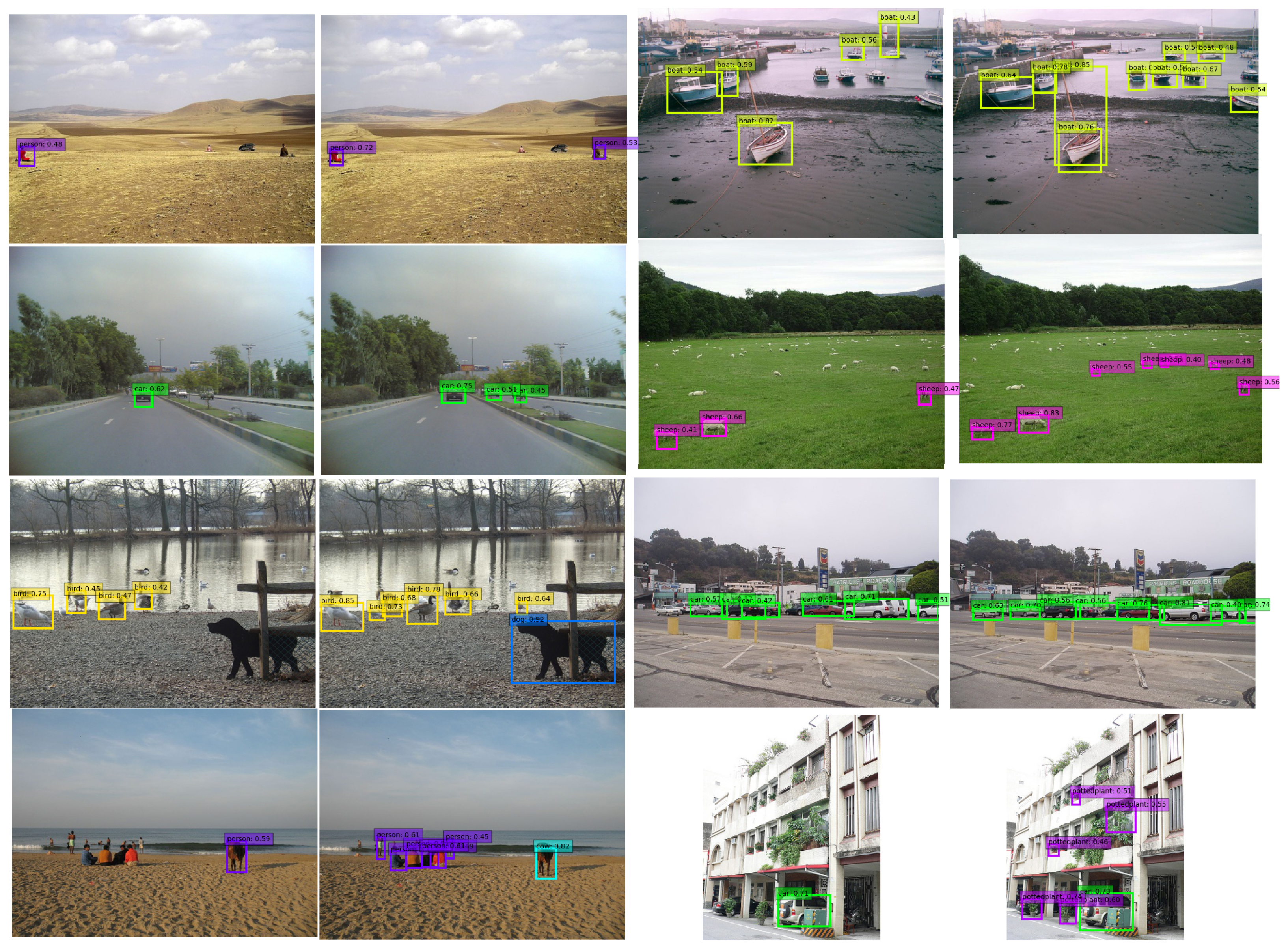
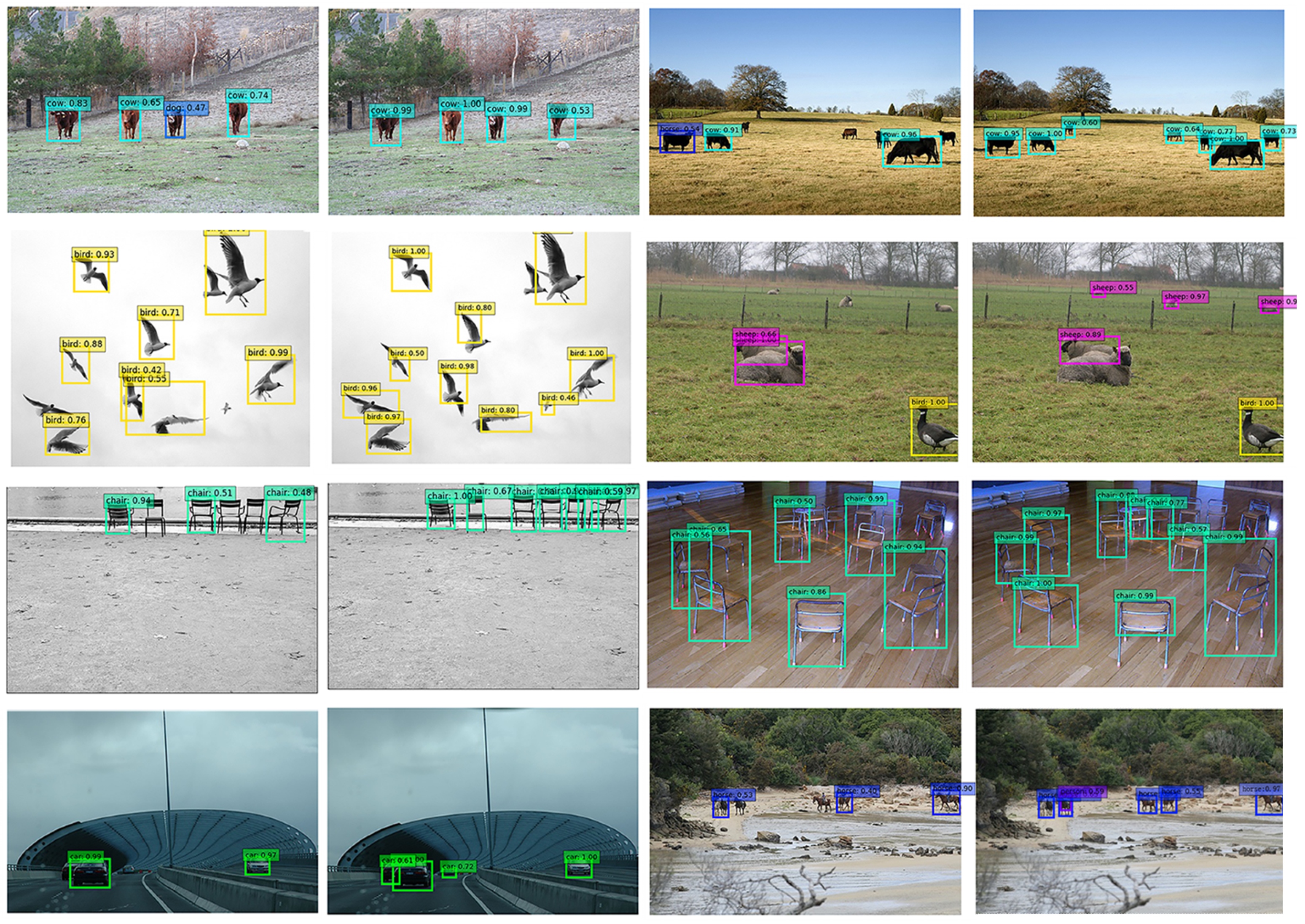
For this test, a total of 106 images containing small objects were selected based on the object scale in the VOC 2007 dataset. The selected objects are small and densely gathered, and most are approximately 1/10 of the image size in scale. In total, the images contain 960 ground-truth objects. Comparisons are presented between the Multi-view YOLO and classical YOLO methods and between the Multi-view SSD and classical SSD methods. Notably, an updated version of YOLO has also been released: YOLOv2 [27]. YOLOv2 has a detection speed of 67 fps on a single Nvidia Titan X graphics card and a mAP of 78.6% on the VOC 2007 test set. To obtain a rich set of comparison results, experiments were conducted on YOLO, YOLOv2, and SSD. The selected object classes include aero, bird, boat, bottle, car, chair, cow, dog, horse, person, potted plant and sheep. By synthetically considering the two aspects of object confidence and object number, the YOLO detection threshold was set to 0.2, and the detection thresholds for both YOLOv2 and SSD were set to 0.4. Typical detection results are shown in Figure 5, Figure 6 and Figure 7.

Figure 5, Figure 6 and Figure 7 show that for small object detection, the multi-view methods exhibit the following three characteristics compared with the classical methods. First, the multi-view methods detect more objects; second, they achieve greater confidence when recognizing the same object; and third, they can correctly identify objects that are incorrectly identified by the classical methods. Classical YOLO did not detect objects in ten images, whereas Multi-view YOLO did not detect objects in only two images. Classical YOLOv2 did not detect objects in four images, and classical SSD did not detect objects in six images, whereas Multi-view YOLOv2 and Multi-view SSD successfully detected objects in all images. These results show that the multi-view methods achieve better performance in small object detection.

Next, the performances of the multi-view methods and the corresponding classical methods will be quantitatively evaluated based on object retrieval ability and detection accuracy.

4.2. Comparison of Object Retrieval Ability

To evaluate the retrieval abilities of the methods, their ability to retrieve objects in each image was first assessed, and the average value of these results was then calculated. Usually, the retrieval ability is assessed using the F-measure, which is the weighted average of the precision and recall and is expressed as follows:

$$F=\frac{(a^2+1)\times P\times R}{a^2\times (P+R)}$$

(7)

where $P$ is the precision, $R$ is the recall, and $a$ is the weight, which is usually set to 1.

For the 106 images considered in this study, the object retrieval abilities of the multi-view methods and the corresponding classical methods are compared in Figure 8, Figure 9 and Figure 10.

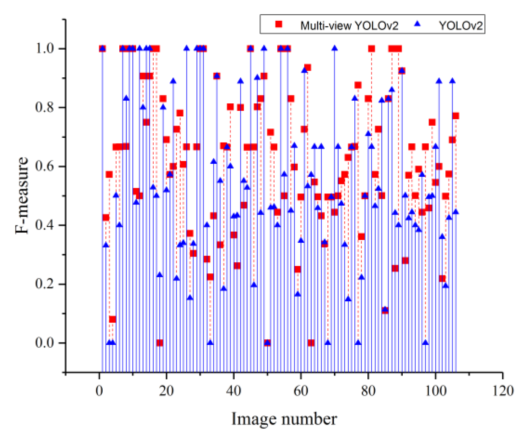
Figure 8, Figure 9 and Figure 10 show that the retrieval abilities of the multi-view methods are mostly higher than those of the classical methods. When calculated as the average retrieval results for all 106 images, the AF (average F-measure) scores of Multi-view YOLO and classical YOLO are 0.496 and 0.319, respectively; the AFs of Multi-view YOLOv2 and classical YOLOv2 are 0.621 and 0.561, respectively; and the AFs of Multi-view SSD and classical SSD are 0.729 and 0.560, respectively. In Figure 8, Figure 9 and Figure 10, a zero point on a curve represents an F-measure value of zero for the corresponding image, which means that the model retrieved no objects that satisfied the retrieval condition. An F-measure value of zero is observed in two situations: when no object is detected in the image and when none of the objects in the detection results satisfies the IoU (Intersection over Union) condition (IoU > 0.5). Corresponding to the first situation, classical YOLO detected no objects in images 3, 33, 36, 46, 68, 74, 89, 95, 97, and 104; Multi-view YOLO detected no objects in images 6 and 97; classical YOLOv2 detected no objects in images 3, 4, 33 and 68; and classical SSD detected no objects in images 6, 32, 46, 56, 71, and 97. Corresponding to the second situation, none of the objects detected by classical YOLO satisfies the IoU condition in images 6, 12, 16, 17, 24, 30, 31, 41, 42, 50, 62, 65, 71, 77, 78, 79, 84, 94, and 96, and the same is true of the objects detected by Multi-view YOLO in images 4, 17, 33, 36, 50, 78, and 94; by classical YOLOv2 in images 50, 77 and 97; by Multi-view YOLOv2 in images 18, 50 and 63; and by classical SSD in images 26, 29, and 50. However, Multi-view SSD successfully retrieved objects in all images. When the above results are combined, classical YOLO has twenty-nine zero points, Multi-view YOLO has nine zero points, classical YOLOv2 has seven zero points, Multi-view YOLOv2 has three zero points, classical SSD has nine zero points, and Multi-view SSD has no zero points. Therefore, the multi-view methods demonstrate better retrieval abilities for small objects than the classical methods do.

4.3. Comparison of Object Detection Accuracy

In object detection, the mAP (mean average precision) metric is typically adopted to evaluate the detection accuracy. For the 106 images introduced above, the mAP values of the classical methods and the corresponding multi-view methods were calculated with the confidence thresholds for YOLO, YOLOv2 and SSD set to 0.2, 0.4 and 0.4, respectively. The results are shown in

Table 2. Small object detection results for regression-based methods on the VOC 2007 dataset.

Method	mAP (%)	AP (%)
		Aero	Bird	Boat	Bottle	Car	Chair	Cow	Dog	Horse	Person	Plant	Sheep
YOLO	24.3	20.2	19.9	7.4	3.9	29.8	19.4	44.2	37.2	/	24.3	20.3	40.6
Multi-view YOLO	38.6	46.9	32.0	34.6	20.5	52.4	39.7	39.7	43.1	/	26.6	30.2	59.3
YOLO*	17.9	18.9	12.6	3.5	3.3	22.1	14.7	28.9	30.2	/	14.9	16.4	31.1
Multi-view YOLO*	30.0	44.1	20.3	16.5	17.2	38.9	30.2	41.5	35.0	/	16.3	24.4	45.4
YOLOv2	48.8	40.0	40.0	38.2	31.5	65.4	52.0	75.4	51.9	28.6	55.8	39.1	68.1
Multi-view YOLOv2	56.2	68.1	40.7	50.1	49.4	80.1	57.9	71.4	71.0	31.4	56.5	32.6	65.3
YOLOv2*	34.7	37.5	25.4	18.2	26.6	48.5	39.5	49.3	42.2	11.1	34.3	31.6	52.2
Multi-view YOLOv2*	40.6	64.1	25.9	23.9	41.7	59.4	44.0	46.7	57.7	12.2	34.7	26.3	50.0
SSD	51.3	65.6	61.2	62.0	18.2	72.1	44.7	59.8	55.2	28.6	53.6	28.8	66.1
Multi-view SSD	64.4	72.9	66.2	72.9	27.0	87.5	66.1	80.5	66.2	54.3	59.2	45.2	75.2
SSD*	36.3	61.8	38.9	29.6	15.6	53.4	34.0	39.1	44.8	11.1	32.9	23.3	50.6
Multi-view SSD*	45.3	68.6	42.1	34.8	22.8	65.0	50.2	52.7	53.8	21.1	36.3	36.5	59.9

¹ Note: An asterisk (“*”) is used to mark object detection results obtained when difficult objects, which are difficult even for experts to recognize when manually labeling the ground-truth objects, are included.

² Note: An underline (“__”) is used to mark the detection results of multi-view methods.

.

Table 2 shows that the mAP scores of the multi-view methods are higher than those of the classical methods in every object class. When difficult objects are not included, the mAP of Multi-view YOLO is 38.6%, which is higher than that of classical YOLO by 14.3%; the mAP of Multi-view YOLOv2 is 56.2%, which is higher than that of the classical YOLOv2 by 7.4%; and the mAP of Multi-view SSD is 64.4%, which is higher than that of classical SSD by 13.1%. When difficult objects are included, the mAP of Multi-view YOLO is 30.0%, which is higher than that of classical YOLO by 12.1%; the mAP of Multi-view YOLOv2 is 40.6%, which is higher than that of classical YOLOv2 by 5.9%; and the mAP of Multi-view SSD is 45.3%, which is higher than that of classical SSD by 9.0%. Hence, the multi-view methods achieve higher accuracy than the classical models for small object detection. However, neither the classical YOLO method nor the Multi-view YOLO method correctly detects horses because horse images are erroneously identified as cows; this behavior is related to the training of the YOLO model. Thus, in Table 2, the mAP scores of both classical YOLO and Multi-view YOLO do not include results for the horse class; however, this omission does not affect the algorithm performance comparison.

The above experimental results indicate that the multi-view approach proposed in this paper enables a better retrieval capability and a higher detection accuracy for small object detection than can be achieved using the classical models.

4.4. Comparisons of Detection Performance between Multi-View Methods and State-of-the-Art Methods Based on Region Proposals

In consideration of the detection results, Multi-view YOLOv2 and Multi-view SSD were chosen for comparison with state-of-the-art methods based on region proposals, including Faster RCNN, R-FCN, and SPP-Net. The mAPs of Faster RCNN, R-FCN, and SPP-Net with a confidence threshold of 0.4 are shown in

Table 3. Small object detection results for region-proposal-based methods on the VOC 2007 dataset.

Method	mAP (%)	AP (%)
		Aero	Bird	Boat	Bottle	Car	Chair	Cow	Dog	Horse	Person	Plant	Sheep
Faster RCNN (VGG)	66.1	74.2	59.2	67.7	73.7	85.2	48.7	76.0	69.1	23.8	73.9	56.2	85.6
Faster RCNN (VGG)*	47.8	69.8	37.6	32.3	62.1	63.2	37.0	49.7	56.2	9.3	45.4	45.4	65.5
RFCN	60.9	67.3	66.1	51.8	46.1	68.7	47.6	77.5	83.4	37.1	72.8	30.7	81.5
RFCN *	43.5	63.4	42.0	24.7	38.9	51.0	36.2	50.7	67.8	14.4	44.7	24.9	63.4
SPP-net	29.8	42.6	32.6	27.5	11.9	45.1	26.2	54.7	10.3	14.3	34.5	15.3	42.7
SPP-net *	21.3	40.1	20.7	13.1	10.0	33.5	19.9	35.8	10.4	5.6	21.2	12.3	32.7

¹ Note: An asterisk (“*”) is used to mark object detection results obtained when difficult objects, which are difficult even for experts to recognize when manually labeling the ground-truth objects, are included.

.

As seen from the table, regardless of whether difficult objects are included, the mAPs of Faster RCNN and R-FCN are much higher than those of YOLOv2 and SSD. However, the performance gap is greatly reduced for Multi-view YOLOv2 and Multi-view SSD. Explicit comparisons of detection performance between the multi-view methods and the state-of-the-art region-proposal-based methods are shown in

Table 4. Small object detection performance on the VOC 2007 dataset.

Method	Multi-View YOLOv2	Multi-View SSD	Faster RCNN (VGG)	RFCN	SPP-net
mAP (%)	56.2	64.4	66.1	60.9	29.8
Run time (sec/img)	0.09	0.10	0.23	0.20	0.42

.

The timing results were evaluated on a single Nvidia Titan X graphics card. Table 4 shows that the detection speeds of Multi-view YOLOv2 and Multi-view SSD are faster than those of the region-proposal-based methods. And Multi-view SSD is comparable to faster RCNN in detection accuracy, and run much faster than faster RCNN. When the mAP and run time results are considered simultaneously, Multi-view SSD exhibits the best detection performance in small object detection among all compared methods.

Therefore, the proposed multi-view approach is an effective means of improving the performance of regression-based methods for small object detection. Although this approach somewhat increases the time required for detection, multi-view methods based on regression still have a speed advantage over state-of-the-art methods based on region proposals.

5. Conclusions

The disadvantage of deep learning object detection model based on regression in small object detection is for the reason that the details of high level feature map remain little. So, we have the idea of increasing the feature response of different image regions in order to improve the detection performance. Here, we proposed the multi-view method to enhance the feature information by producing more response in the same level feature map.

This paper proposes a multi-view object detection approach for small object detection. Experiments were performed using a small object dataset selected from the VOC 2007 dataset. The experimental results show that in terms of object retrieval capability, Multi-view YOLO, Multi-view YOLOv2, and Multi-view SSD achieve AF scores that are higher than those of their classical counterparts by 0.177, 0.06, and 0.169, respectively. Moreover, in terms of the detection accuracy, when difficult objects are not included, the mAP scores of the multi-view methods are higher than those of the classical methods by 14.3%, 7.4%, and 13.1%, respectively. The results show that both the object retrieval abilities and detection accuracies of multi-view methods are better than those of the corresponding classical methods, verifying the validity of the proposed approach. In addition, the applicability of the proposed multi-view approach is not restricted to YOLO and SSD; it can be applied in combination with some other regression-based detection models. This will further improve the performance of the regression-based detection models in small object detection. Therefore, the multi-view approach proposed in this paper offers an excellent solution for improving the small object detection capabilities of regression-based detection models. In our future work, the overall image information will be combined with the multi-view paradigm to enhance the algorithm’s performance.

References

- Erhan, D.; Szegedy, C.; Toshev, A.; Anguelov, D. Scalable object detection using deep neural networks. In Proceedings of the IEEE Conference on Computer Vision and Pattern Recognition, Columbus, OH, USA, 24–27 June 2014; pp. 2147–2154. [Google Scholar]
- Borji, A.; Cheng, M.M.; Jiang, H.; Li, J. Salient object detection: A benchmark. IEEE Trans. Image Process. 2015, 24, 5706–5722. [Google Scholar] [CrossRef] [PubMed]
- Jeong, Y.N.; Son, S.R.; Jeong, E.H.; Lee, B.K. An Integrated Self-Diagnosis System for an Autonomous Vehicle Based on an IoT Gateway and Deep Learning. Appl. Sci. 2018, 7, 1164. [Google Scholar] [CrossRef]
- Wu, X.; Huang, G.; Sun, L. Fast visual identification and location algorithm for industrial sorting robots based on deep learning. Robot 2016, 38, 711–719. [Google Scholar]
- Merlin, P.M.; Farber, D.J. A parallel mechanism for detecting curves in pictures. IEEE Trans. Comput. 1975, 100, 96–98. [Google Scholar] [CrossRef]
- Singla, N. Motion detection based on frame difference method. Int. J. of Inf. Comput. Tech. 2014, 4, 1559–1565. [Google Scholar]
- Lee, D.S. Effective Gaussian mixture learning for video background subtraction. IEEE Trans. Pattern Anal. Mach. Intell. 2005, 27, 827–832. [Google Scholar] [PubMed] [Green Version]
- Horn, B.K.P.; Schunck, B.G. Determining optical flow. Artif. Intell. 1981, 17, 185–203. [Google Scholar] [CrossRef] [Green Version]
- Viola, P.; Jones, M. Rapid object detection using a boosted cascade of simple features. In Proceedings of the IEEE Conference on Computer Vision and Pattern Recognition, Kauai, HI, USA, 8–14 December 2001; pp. 511–518. [Google Scholar]
- Felzenszwalb, P.F.; Girshick, R.B.; McAllester, D.; Ramanan, D. Object detection with discriminatively trained part-based models. IEEE Trans. Pattern Anal. Mach. Intell. 2010, 32, 1627–1645. [Google Scholar] [CrossRef] [PubMed]
- Lowe, D.G. Distinctive image features from scale-invariant keypoints. Int. J. Comput. Vis. 2004, 60, 91–110. [Google Scholar] [CrossRef]
- Dalal, N.; Triggs, B. Histograms of oriented gradients for human detection. In Proceedings of the IEEE Conference on Computer Vision and Pattern Recognition, Boston, MA, USA, 8–10 June 2015; pp. 886–893. [Google Scholar]
- Panning, A.; Al-Hamadi, A.K.; Niese, R.; Michaelis, B. Facial expression recognition based on Haar-like feature detection. Pattern Recognit Image Anal. 2008, 18, 447–452. [Google Scholar] [CrossRef]
- Burges, C.J.C. A tutorial on support vector machines for pattern recognition. Data Min. Knowl. Discov. 1998, 2, 121–167. [Google Scholar] [CrossRef]
- Zhu, J.; Zou, H.; Rosset, S.; Hastie, T. Multi-class adaboost. Stat. Interface 2009, 2, 349–360. [Google Scholar]
- Kong, T.; Yao, A.; Chen, Y.; Sun, F. HyperNet: Towards accurate region proposal generation and joint object detection. In Proceedings of the IEEE Conference on Computer Vision and Pattern Recognition, Las Vegas, NV, USA, 26 June–1 July 2016; pp. 845–853. [Google Scholar]
- Girshick, R.; Donahue, J.; Darrell, T.; Malik, J. Rich feature hierarchies for accurate object detection and semantic segmentation. In Proceedings of the IEEE Conference on Computer Vision and Pattern Recognition, Columbus, OH, USA, 24–27 June 2014; pp. 580–587. [Google Scholar]
- He, K.; Zhang, X.; Ren, S.; Sun, J. Spatial pyramid pooling in deep convolutional networks for visual recognition. In Proceedings of the European Conference on Computer Vision, Zurich, Switzerland, 6–12 September 2014; pp. 346–361. [Google Scholar]
- Girshick, R. Fast r-cnn. In Proceedings of the IEEE International Conference on Computer Vision, Boston, MA, USA, 8–10 June 2015; pp. 1440–1448. [Google Scholar]
- Ren, S.; He, K.; Girshick, R.; Sun, J. Faster r-cnn: Towards real-time object detection with region proposal networks. In Proceedings of the International Conference on Neural Information Processing Systems, Cambridge, MA, USA, 7–12 December 2015; pp. 91–99. [Google Scholar]
- Li, Y.; He, K.; Sun, J. R-fcn: Object detection via region-based fully convolutional networks. In Proceedings of the International Conference on Neural Information Processing Systems, Barcelona, Spain, 9 December 2016; pp. 379–387. [Google Scholar]
- Redmon, J.; Divvala, S.; Girshick, R.; Farhadi, A. You only look once: Unified, real-time object detection. In Proceedings of the IEEE Conference on Computer Vision and Pattern Recognition, Las Vegas, NV, USA, 26 June–1 July 2016; pp. 779–788. [Google Scholar]
- Liu, W.; Anguelov, D.; Erhan, D.; Szegedy, C.; Reed, S.; Fu, C.; Berg, A.C. SSD: Single shot multibox detector. In Proceedings of the European Conference on Computer Vision, Amsterdam, The Netherlands, 8–16 October 2016; pp. 21–37. [Google Scholar]
- Eggert, C.; Zecha, D.; Brehm, S.; Lienhart, R. Improving Small Object Proposals for Company Logo Detection. In Proceedings of the 2017 ACM on International Conference on Multimedia Retrieval, Bucharest, Romania, 6–9 June 2017; pp. 167–174. [Google Scholar]
- Fu, C.; Liu, W.; Ranga, A.; Tyagi, A.; Berg, A.C. DSSD: Deconvolutional Single Shot Detector. 2017. 1701.06659. Cornell University. Available online: https://arxiv.org/abs/1701.06659 (accessed on 23 July 2018).
- Cai, Z.; Fan, Q.; Feris, R.S.; Vasconcelos, N. A unified multi-scale deep convolutional neural network for fast object detection. In Proceedings of the European Conference on Computer Vision, Amsterdam, Netherlands, 8–16 October; pp. 354–370.
- Redmon, J.; Farhadi, A. YOLO9000: Better, faster, stronger. 2016. 1612.08242. Cornell University. Available online: https://arxiv.org/abs/1612.08242 (accessed on 23 July 2018).
Figure 1.
Imaging principle of the human eye.
Figure 2.
Multi-view segmentation.
Figure 3.
Model for multi-view object detection.
Figure 4.
Evaluation of adjacent boundary lines in multiple views.
Figure 5.
Comparisons of small object detection results between the classical You Only Look Once (YOLO) method (the first and third columns) and the Multi-view YOLO method (the second and fourth columns).
Figure 6.
Comparisons of small object detection results between the classical YOLOv2 method (the first and third columns) and the Multi-view YOLOv2 method (the second and fourth columns).
Figure 7.
Comparisons of small object detection results between the classical SSD method (the first and third columns) and the Multi-view SSD method (the second and fourth columns).
Figure 8.
Comparison of the object retrieval abilities of the Multi-view YOLO and classical YOLO methods.
Figure 9.
Comparison of the object retrieval abilities of the Multi-view YOLOv2 and classical YOLOv2 methods.
Figure 10.
Comparison of the object retrieval abilities of the Multi-view SSD and classical SSD methods.