Article

Single-Class Data Descriptors for Mapping Panax notoginseng through P-Learning

School of Geodesy and Geomatics, Wuhan University, Wuhan 430079, China
*
Author to whom correspondence should be addressed.
Appl. Sci. 2018, 8(9), 1448; https://doi.org/10.3390/app8091448
Submission received: 16 August 2018 / Revised: 20 August 2018 / Accepted: 21 August 2018 / Published: 24 August 2018

Abstract

:
Machine learning-based remote-sensing techniques have been widely used for the production of specific land cover maps at a fine scale. P-learning is a collection of machine learning techniques for training the class descriptors on the positive samples only. Panax notoginseng is a rare medicinal plant, which also has been a highly regarded traditional Chinese medicine resource in China for hundreds of years. Until now, Panax notoginseng has scarcely been observed and monitored from space. Remote sensing of natural resources provides us new insights into the resource inventory of Chinese materia medica resources, particularly of Panax notoginseng. Generally, land-cover mapping involves focusing on a number of landscape classes. However, sometimes a subset or one of the classes will be the only part of interest. In term of this study, the Panax notoginseng field is the right unit class. Such a situation makes single-class data descriptors (SCDDs) especially significant for specific land-cover interpretation. In this paper, we delineated the application such that a stack of SCDDs were trained for remote-sensing mapping of Panax notoginseng fields through P-learning. We employed and compared SCDDs, i.e., the simple Gaussian target distribution, the robust Gaussian target distribution, the minimum covariance determinant Gaussian, the mixture of Gaussian, the auto-encoder neural network, the k-means clustering, the self-organizing map, the minimum spanning tree, the k-nearest neighbor, the incremental support vector data description, the Parzen density estimator, and the principal component analysis; as well as three ensemble classifiers, i.e., the mean, median, and voting combiners. Experiments demonstrate that most SCDDs could achieve promising classification performance. Furthermore, this work utilized a set of the elaborate samples manually collected at a pixel-level by experts, which was intended to be a benchmark dataset for the future work. The measuring performance of SCDDs gives us challenging insights to define the selection criteria and scoring proof for choosing a fine SCDD in mapping a specific landscape class. With the increment of remotely sensed satellite data of the study area, the spatial distribution of Panax notoginseng could be continuously derived in the local area on the basis of SCDDs.

1. Introduction

Traditional Chinese medicine (TCM) [1] originated in ancient China and has evolved over thousands of years as the only health care and disease healing [2]. A long time before the birth of modern Western medicine, traditional medicinal recipes were handed down orally generation by generation in many parts of the world [3]. Given that TCM is a practical medicine built on experience, and has been mainly practiced and researched in China [4,5], the essence of TCM has always been the most advanced and experienced medicine in the world [6]. Moreover, scientists proved that TCM can coexist with Western medicine [3,7]. Geoherb is a type of Chinese herb with a geographical indication corresponding to a specific geographical location or origin, which has a certification that the product possesses certain qualities, and its production will be protected by intellectual property rights law [8,9]. Compared to the herbal resources produced in other areas, the quality and efficacy of geoherbs are much better [10]. As a highly-regarded TCM resource and a rare kind of geoherb in China [11,12], Panax notoginseng (see Figure 1) has been cultivated for more than 400 years in the south-west region of China [13], especially in Wenshan Prefecture, Yunnan province. The conventional methods of TCM resource surveys mainly focus on the qualitative description of species rather than the natural storage or dynamic changes of the planting fields, resulting in a problematic situation that TCM resources appear difficult to monitor over time, which is not conducive to the sustainable development of TCM [14]. In the past few decades, a resource census of TCM has been carried out three times (e.g., 1960–1962, 1969–1973, and 1983–1987). Until 2009, the government of China proposed “To carry out a nationwide census of TCM resources, strengthen the monitoring of TCM resources and the construction of an information network” [15]. Furthermore, the State Council of China highlighted “Strengthening the landscape-scale dynamic monitoring and protection of TCM” [16] again. From 2011, the government of China planned to conduct the fourth national census of TCM resources, and remote-sensing techniques were regarded as the core-key technologies for surveying and monitoring TCM resources in a large area. The inheritance, innovation, modernization, and internationalization of TCM would be the four basic tasks for a considerable period of time [17,18].
Remote-sensing techniques have been applied to monitor land cover at a range of spatial and temporal scales, in order to satisfy a range of scientific and practical requirements [19,20,21]. In particular, remote-sensing mapping is an efficient technique to acquire spatial and temporal cropland information repeatedly and consistently [22,23]. In many cases, remotely-sensed data are utilized to derive landscape information on a specific land-cover class of interest [24]. The ability to map and monitor land-cover types and their dynamics for diverse applications has been enhanced by the availability and constantly increased coverage, of satellite images [25,26]. Many problems are encountered in mapping land cover from remotely sensed data by a classification analysis or landscape class description [27] in order to quantify the relationships among all the pixels in an image, such as similarities or differences in spectra signature or spatial texture [22], and extract land cover classes from remote-sensing images [28,29,30]. The application of remote-sensing techniques plays a significant role in the quantitative resource survey of TCM, particularly in exploring monitoring abilities for the sustainable utilization and bio-diversity protection of Chinese materia medica resources in macrocosm. Under the prerequisite that remote-sensing techniques provide up-to-date landscape surveying at a fine scale [31], one of the motivations for this work comes from the fact that only a single class of interest is involved in a mapping task.
Recently, there has been a number of applications [32], i.e., geological products [33], vegetation indices [34], aerosol products [35], ocean data products [36], dust source identification [37], and crops identification [38] in remote-sensing based on machine learning techniques. In this study, we present an original innovation to apply most of the available single-class data descriptors (SCDDs) through P-learning to conduct mapping of Panax notoginseng fields. After that, the work of measuring performance will give us profound insights into defining the selection criteria and scoring proof for choosing a fine SCDD. As such, the introduction of SCDDs for remote-sensing mapping of Panax notoginseng fields will be helpful to promoting the development of a Panax notoginseng resource inventory and dynamic monitoring towards the quantitative direction. Attributing to the standardized cultivation technique of good agricultural practice (GAP) [39], or so-called controlled-environment agriculture using shade houses provide a distinct image texture to interpret Panax notoginseng fields visually [40]. Additionally, due to only Panax notoginseng fields being the target class, the task of mapping Panax notoginseng fields becomes a specific typology of land-cover classification, which could be regarded as a problem of single-class data description or a special type of one-class classification [41]. SCDDs are the appealing alternatives to the conventional supervised classifiers because they can be trained with only the target training samples [42]. These kinds of algorithms have emerged to only require training samples from the target class, which are referred to as P-learning [43]. Notice that the single class meant no more than one landscape class, and the P-learning based class description may depict the sight that no negative samples are used for training. Such a classification approach aims to identify only one landscape class of interest regardless of the other classes presented in the study area [44]. In the case of single-class data description, we always face an imbalanced binary classification [45,46] including (1) the positive class (i.e., Panax notoginseng fields); and (2) the negative class (i.e., the other classes). In this case, the positive class is assumed to be sampled well, while the other classes may be sampled very sparsely or totally absent. When no samples of the other classes are available, most classification errors (e.g., false negative) cannot be estimated [47]. In addition, the procedure that trains an accurate SCDD is challenging, particularly in the face of a large number of unlabeled samples; or say, only a small class or relatively few training samples are available [42]. Therefore, it might be very expensive to collect the negative samples which are so abundant that a good sampling seems elusive. Although this was an extreme case, we carefully designed the training and test sets, which were composed of the qualified positive and negative samples. Note that if we want to improve the overall performance of the numerous classifiers which may differ in complexity, a combination of these classifiers will always be a viable solution [48].
Regarding another motivation of this work with respect to TCM, the quality control of TCM remains a significant issue that affects medicinal herbs, formulations, and even TCM practice. Due more to the lax enforcement of standards [49], resulting in the diminishing popularity of TCM rather than a failure of remedies, particularly, the patchy regulation has led to inconsistent herb quality, unqualified practitioners, unsubstantiated claims for secret formulas, and both deliberate and inadvertent mislabeling and adulteration, sometimes with fatal consequences. Considering Panax notoginseng is a vulnerable crop which has a serious succession cropping obstacle [50], consequently the continuous planting of the same crop in the same field will lead to the decrease of yield and quality. In order to promote the quality of production, it is crucial to monitor the spatial planting patterns of Panax notoginseng fields, such as crop rotation [51,52]. The planting pattern implies standardized planting with the specific crop structure and spatio-temporal configuration in the same field for a specific region under the particular natural resource and socio-economic conditions [53,54] so as to realize the sustainable utilization of agricultural resources and crop yield. Until now, the concrete planting pattern changes of Panax notoginseng are still poorly known. To the best of our knowledge, until now no such work has been done which, on the one hand, enriches the approaches to monitor spatial planting pattern changes of the perennial ginseng from space; on the other hand, employs SCDDs for mapping Panax notoginseng.
Our studies on mapping Panax notoginseng aim to provide fruitful information for studies on the quality assurance of TCM production, precision farming, the construction of agro-ecosystems, sustainable development, and the protection of the biodiversity of Panax notoginseng. Furthermore, determining the planting area of Panax notoginseng is an important part of obtaining more accurate information about annual yield and natural storage, except for mapping the spatial distribution. The current study, which involves mapping the planting parcels of Panax notoginseng at a 30 m spatial resolution, has three aims: (1) mapping Panax notoginseng fields through a stack of SCDDs as the future technical milestone for planting pattern analysis; (2) evaluating the abilities of SCDDs in identifying small Panax notoginseng fields in the complex agricultural landscapes; and (3) providing the potential possibilities for monitoring the planting pattern changes of Panax notoginseng fields, further giving us new insights into the planting pattern transitions of the perennial ginseng in macrocosm. The case study area is located in Wenshan City of China, which is characterized by a distinctive crop rotation agricultural system. The highlights of this study include: (1) striving for the research of the landscape-scale remote-sensing interpretation of TCM resources for the first time; (2) employing a stack of SCDDs with a comparative perspective to conduct mapping of Panax notoginseng fields; (3) defining the selection criteria and scoring proof for choosing a most appropriate SCDD; and (4) evaluating the abilities of SCDDs in identifying the fragmented parcels of Panax notoginseng in the complex agricultural landscapes.
The rest of this paper is structured as follows. The description of materials and methods is introduced in Section 2, and the experiments and analysis are presented and discussed in Section 3 and Section 4, respectively. Finally, the conclusions of this work are summarized in Section 5.

2. Materials and Methods

2.1. Study Area and Data

Our study area comprises two independent blocks which are situated in Wenshan City, Wenshan Prefecture, Yunnan Province, in the south-west region of China (see Figure 2). These places mainly lie between longitude 103.71° E–104.46° E and latitude 23.07° N–23.73° N. Wenshan Prefecture is on a plateau, where the temperatures are quite constant throughout the year, with more precipitation during the summer months. Due to its low latitude and tempered by its high elevation, Wenshan Prefecture has a mild, humid, and subtropical climate, particularly suitable for planting Panax notoginseng. This is the reason why Wenshan Prefecture is the specific geographical location and origin of Panax notoginseng (i.e., why it is called a geoherb).
The “sa” and “sb” are two typical square regions. There are 151 × 151 pixels in the image space, respectively, corresponding to an area 20.5209 km2 or equivalent to 2052.09 ha for both. The two blocks have a typical representation of the dense Panax notoginseng fields, upon which mapping Panax notoginseng fields will be carried out using multiple SCDDs. Multi-spectral cloud-free images acquired by the Landsat-8 Operational Land Imager (OLI) at a 30 m spatial resolution were utilized in this study. Their acquisition date was 18 March 2015. Since only one scene (path/row: 128/044) was utilized for the analysis in this study, the atmosphere can be considered to be homogeneous, and therefore the atmospheric correction may be not necessary [41,55]. Note that the planting fields of Panax notoginseng are rather sparse in most cases, and the cloud-free satellite images are not easy to collect because of the special geographical environment (i.e., a mountainous area is often in heavy clouds, refer to Table 1).

2.2. Shadenet Structures

Plastic sheets are used as materials to build the shadenet structure which can be regarded as a micro-scale planting environment and are relatively common [56], having unique characteristics [57], i.e., optical transparency, shade percentages, gas-tightness, and high-reflectivity. Agriculturalists have long known the importance of the planting environment for crop growth, always by manipulating the growing environment to provide a more conducive environment for crop growth. As for Panax notoginseng, sunlight is often modified by shading to provide the more optimal growing environments so as to enhance their production. Therefore, the production of Panax notoginseng takes place within an enclosed growing structure called a shade house. The shade house (see Figure 3) provides the protection and maintains the optimal growing conditions throughout the development of Panax notoginseng. The shade house of Panax notoginseng is a framed structure often covered with the black plastic nets which are made of the polyethylene thread with different shade percentages. It provides a partially-controlled atmosphere and environment by reducing the light intensity and effective heat during daytime to Panax notoginseng grown under the very large plastic sheets.
Additionally, attributed to the standardized cultivation technique of GAP, the shade house provides a distinct spatial texture to interpret the spatial distribution of Panax notoginseng fields in reference to Google Earth historical images based on a calendar, i.e., there are 20 days when the satellite images were captured from 6 March 2013, to 12 December 2015, which is associated with the different sampling sites (see Figure 4), i.e., there are a total of 123 sites in Wenshan City. Polypropylene fabric shade is the dominant shade for field-cultivated Panax notoginseng in Wenshan City. Its black color maintains the proper shade and also forms the distinct texture of the shade net in satellite images, which can be visually interpreted and makes it easier to collect training samples using region of interest (ROI) tools.

2.3. Design Sets

Good classification depends not only on the factors associated with classifiers, but fine design sets also play a significant role in assessing the classification results objectively [58]. There is a non-negligible truth that, if only given positive samples, we cannot estimate most of the classification errors. Therefore, both positive and negative samples are supposed to be prepared for this study. Silva, et al. [41] utilized a manually-collected set of samples of the target class and a random sampling of samples of all classes, to keep the training effort low. In that case, they used the non-pure negative samples under the assumption of which few samples of the target class would be submerged.
In this study, we manually collected the positive (i.e., 1211) and negative (i.e., 8522) samples with a class-wise separability of 1.9918. Subsequently, we prepared three kinds of design sets, i.e., the training set (i.e., 727 positive samples, and 5114 negative samples at a 60% split); test set (484 positive samples, and 3408 negative samples, the remaining 40% split); and validation set (only 51 positive samples for the “sa”, and 94 positive samples for the “sb”); as well as additional reference results (see Figure 5) obtained by the expert processing software. The training and test sets are random subsets of the raw collected samples by splitting operation. Note that once determined, they should be fixed so that all SCDDs could be fairly compared. For a good estimate, the test set should be labeled, randomly drawn from the class of interest, independent from the training set, and as large as possible. The validation set (i.e., only comprising true labels of the positive class) is used for validation and a nominal set. Note that the raw samples covering the whole of Wenshan City are specially designed for training and testing SCDDs. Meanwhile, the true labels for validation set are applied to calculate a representative accuracy (i.e., a correct rate) of the classification results as a final validation.

2.4. Single-Class Data Descriptors (SCDDs)

The SCDD [47] is a trained mapping to predict classes. Additionally, they can be divided into several categories depending on the type of the training data and the discrimination function [59]. For example, the positive samples only (i.e., P-learning) or the positive and unlabeled samples (i.e., PU-learning) [31,59]. In general, for certain SCDDs, the corresponding model can be defined as
h ( x ) = { t a r g e t ,   f ( x ) θ o t h e r ,   f ( x ) > θ ,
or vice versa in the opposite conditions.
The threshold θ is set according to the target error. Formally, each instance is mapped to one element of the set of the positive and negative class labels. In this study, due to only the target class (i.e., Panax notoginseng fields) is the class of interest, and the task of mapping Panax notoginseng fields can be regarded as a specific single-class data description problem. Hence, 10 SCDDs [47], i.e., the simple Gaussian target distribution data description (SGTD coded as c1) [60]; the robust Gaussian target distribution data description (RGTD coded as c2) [60]; the minimum covariance determinant Gaussian data description (MCDG coded as c3) [60]; the mixture of Gaussian data description (MoG coded as c4) [60]; the auto-encoder neural network data description (AENN coded as c6) [61]; the k-means clustering data description (k-means coded as c7) [62]; the self-organizing map data description (SOM coded as c10) [63]; the minimum spanning tree data description (MST coded as c11) [64]; the k-nearest neighbor data description (K-NN coded as c13) [65]; the incremental support vector data description (IncSVDD coded as c17) [66]; the Parzen density estimator data description (PDE coded as c5, which is a known underestimated descriptor) [67]; and the principal component analysis data description (PCA coded as c9, which is known as an overestimated descriptor) [68].
In addition to the SCDDs mentioned above, three ensemble classifiers, i.e., the mean combiner (meanc coded as cmea), the median combiner (medianc coded as cmed), and the voting combiner (votec coded as cvot), taking the mean, median, and vote strategies, respectively. The ensemble-based approach refers to the multiple-classifier system in which the outputs of all member classifiers are combined to derive an accurate classification. We combine the SCDDs which should be accurate but different in an ensemble strategy because each of them can focus on a specific feature or characteristic in the feature space [24]. Thus, a much more flexible and outstanding classifier can be obtained by combining all the strong points of the different SCDDs. There are three strategies of combining the different SCDDs, which are referred to as (1) sequential, (2) parallel, and (3) stacked [47]. Here, the above-enumerated SCDDs (i.e., c1–c17) are computed in the same feature space, and which are typically combined in a stacked way. Notice that, the combining procedure is computationally intensive in the face of many different base classifiers. Thus, the action that prunes the base classifiers according to their performance (i.e., underestimated or overestimated) is inevitable sometimes. In this study, ten SCDDs except for the underestimated and overestimated ones, which are regarded as the qualified member classifiers. The abovementioned SCDDs and combiners have been well implemented with a Matlab toolbox for data description developed and distributed by Dr. David Tax.

2.5. Performance Evaluation

In this study, the error computation and performance evaluation involve several accuracy metrics, i.e., the basic errors (see Table 2), F1 measure, receiver operating characteristics (ROC) curve, area under the ROC curve (AUC) error, cost curve, confusion matrix, and correct rate, which are employed to evaluate the SCDDs in a more comprehensive way. In order to find a good SCDD, four basic errors can be calculated, and two of them have to be minimized, namely the false positives (FP) and false negatives (FN). Hence, we put forward and discuss several representative measures which can reflect the probability that the prediction is informed versus chance. The FN can be estimated on the positive set. In fact, the FN is much harder to estimate when no negative samples are available [47]. If only minimizing the FN will lead to the SCDD which may wrongly label a number of the negative samples as the positive class. In order to avoid such a degenerate solution, the negative samples have to be collected as well. This is the reason why we elaborately prepared the design sets and the reference results for training and testing. Moreover, two other measures, such as precision and recall (i.e., the true positive (TP) rate), are often used in performance evaluation. Finally, a derived performance indicator F1 score can be computed. Note that a good SCDD should have both small rates of the FN and FP.
Due to the error on the positive class can be estimated relatively well, assuming that, a threshold can be set beforehand on the target error for the SCDDs, and then a ROC curve can be obtained by varying this threshold and measuring the error on the negative samples. The ROC graph [69,70] shows how the FP varies for varying the FN, which is a technique for visualizing and selecting the best classifiers based on their performance. The smaller these fractions are, the more the SCDD is to be preferred. Although the ROC graph shows an intuitive metric of the performance of the SCDD, as one side, it is a bit difficult to compare the ROC curves; for another, we want to reduce the ROC curve to a single scalar value representing the expected performance. Thus, the AUC error [71,72] often is taken, and which is computed from the ROC curve, which integrates the fraction TP over varying thresholds (or by varying fraction FP equivalently). The larger the AUC value, the better the SCDD’s performance. That is, the higher values may indicate a better separation between the positive and negative samples. As for the ROC graph [70], there are many thresholds that may be suboptimal. That is, there is another operating point for which at least one of the errors is lower. Nevertheless, this concern can be indicated by a cost curve [73], which will be another method for visualizing the performance of the SCDD. For a varying cost-ratio between both classes, the expected cost is computed. Additionally, once a trained mapping has been determined, we can obtain the sufficient site-specific metrics derived from a confusion matrix (i.e., a binary contingency table for the SCDD). The binary confusion matrix (see Table 2) is a specific table layout that allows the visualization of the performance of the SCDD [74]. Such an error matrix is constructed via classifying a predefined test set or comparing two sets of labels, and which combines the spatial position and quantitative information of the classification results to implement a performance evaluation. What is important is that the very small changes of labels are well reflected in a confusion matrix.

3. Results and Analysis
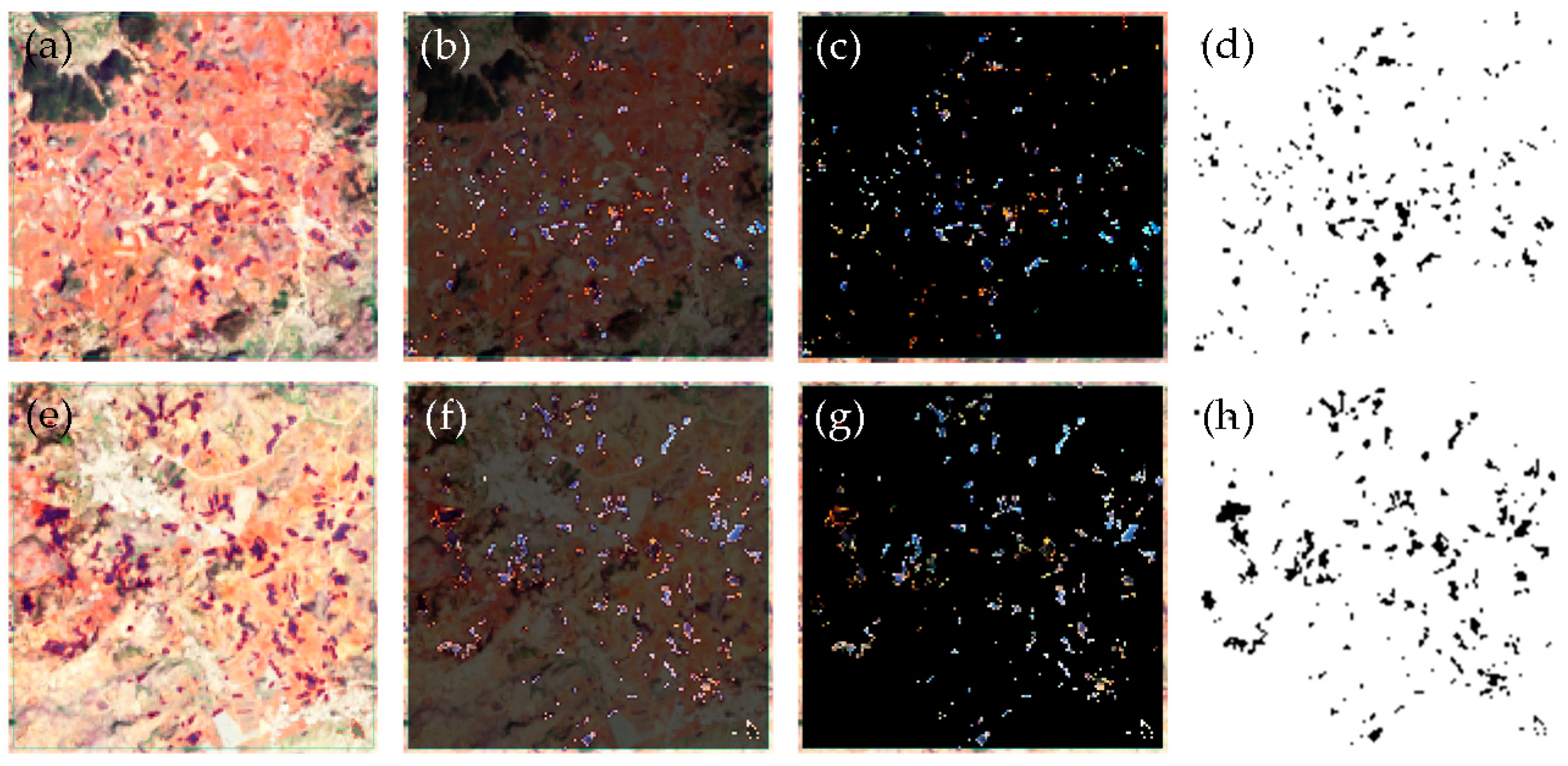
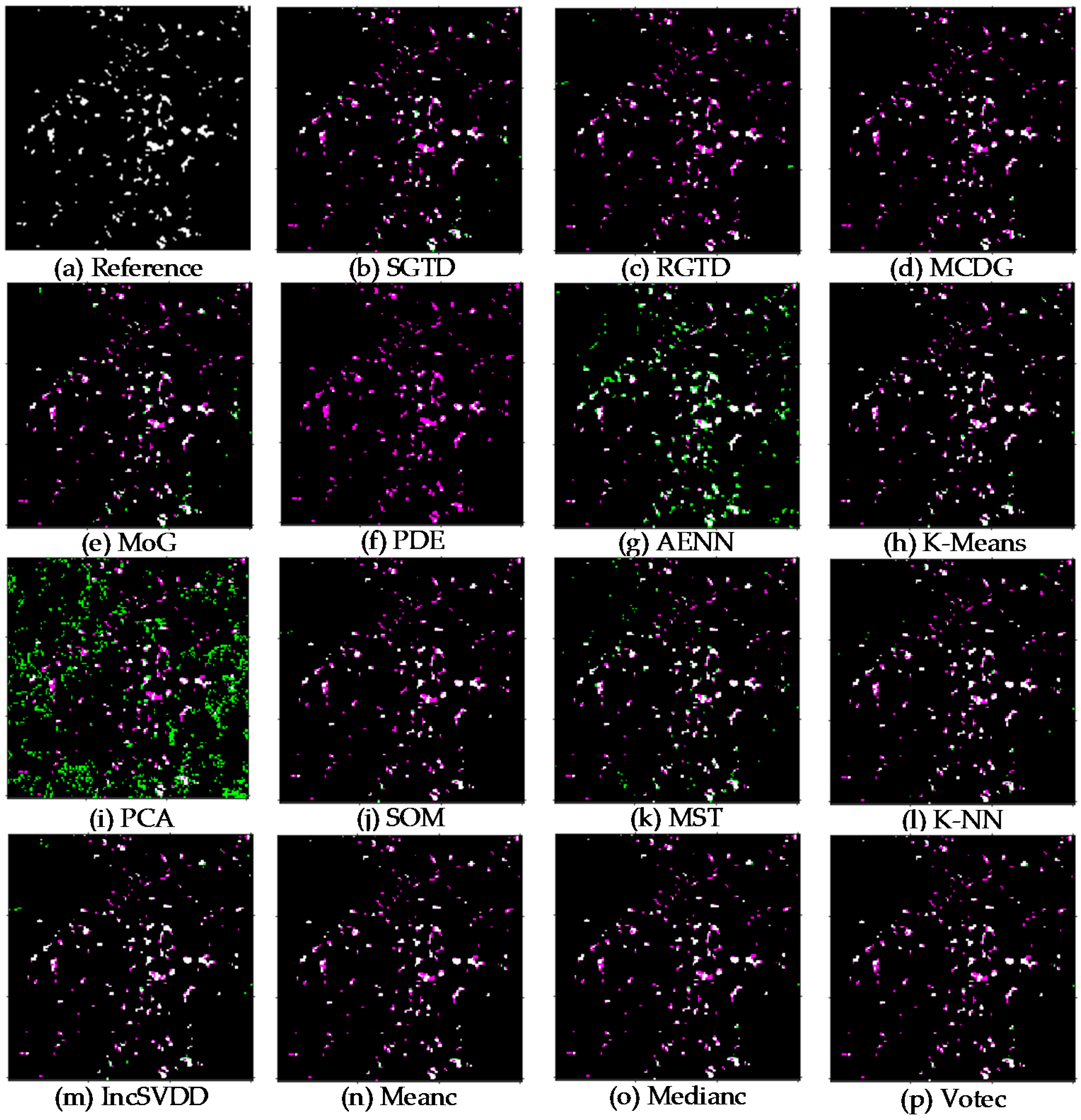
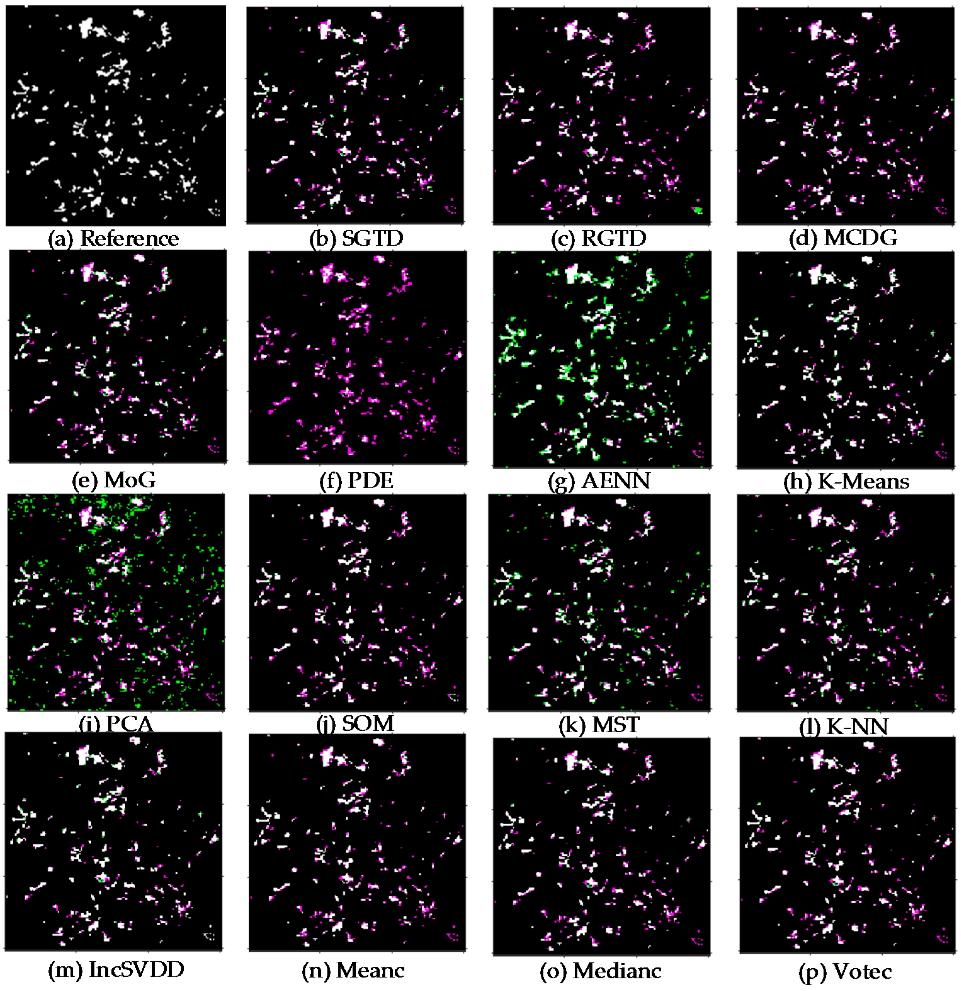
3.1. Resultant Maps

After the SCDDs have been performed, and then the final outputs associated with mapping Panax notoginseng fields can be derived. For one side, we conduct a statistical analysis from a perspective of quantitative evaluation. Besides, we want an intuitive comparison by showing the paired maps which are overlapped in false-color style between the classification and reference maps regarding the spatial distribution of Panax notoginseng fields.
As such, the classification map of each SCDD in comparison with the reference map that can be simultaneously graphed for the “sa” and “sb” (see Figure 6 and Figure 7). By visual inspection, the obvious differences have been observed with respect to the underestimated PDE (see Figure 6 and Figure 7) and the overestimated PCA (see Figure 6 and Figure 7). The heavy magenta patches mean seriously underestimated, while a large number of green patches mean severely overestimated. The majority of the rest of the SCDDs arise from the predominately magenta and slightly green patches, which mean underestimated. Meanwhile, AENN is different (see Figure 6 and Figure 7). Notice that the error threshold on the positive class is set by a default float value of 0.1 for all SCDDs. In a number of clusters a default integer value of 2 will be acceptable because only two classes are available (i.e., the positive and negative class). Additionally, the number of components is set to 5 in terms of PCA.

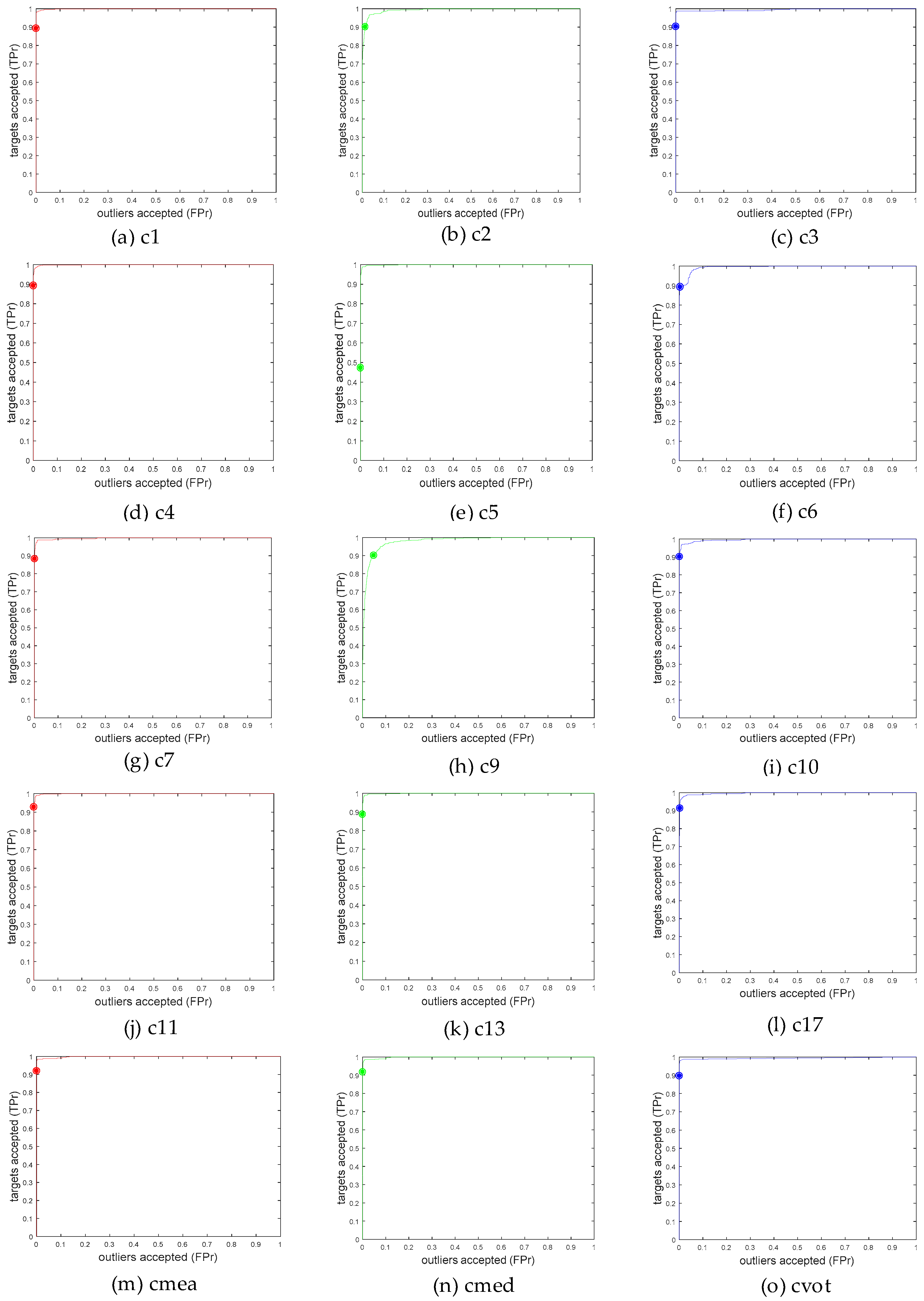
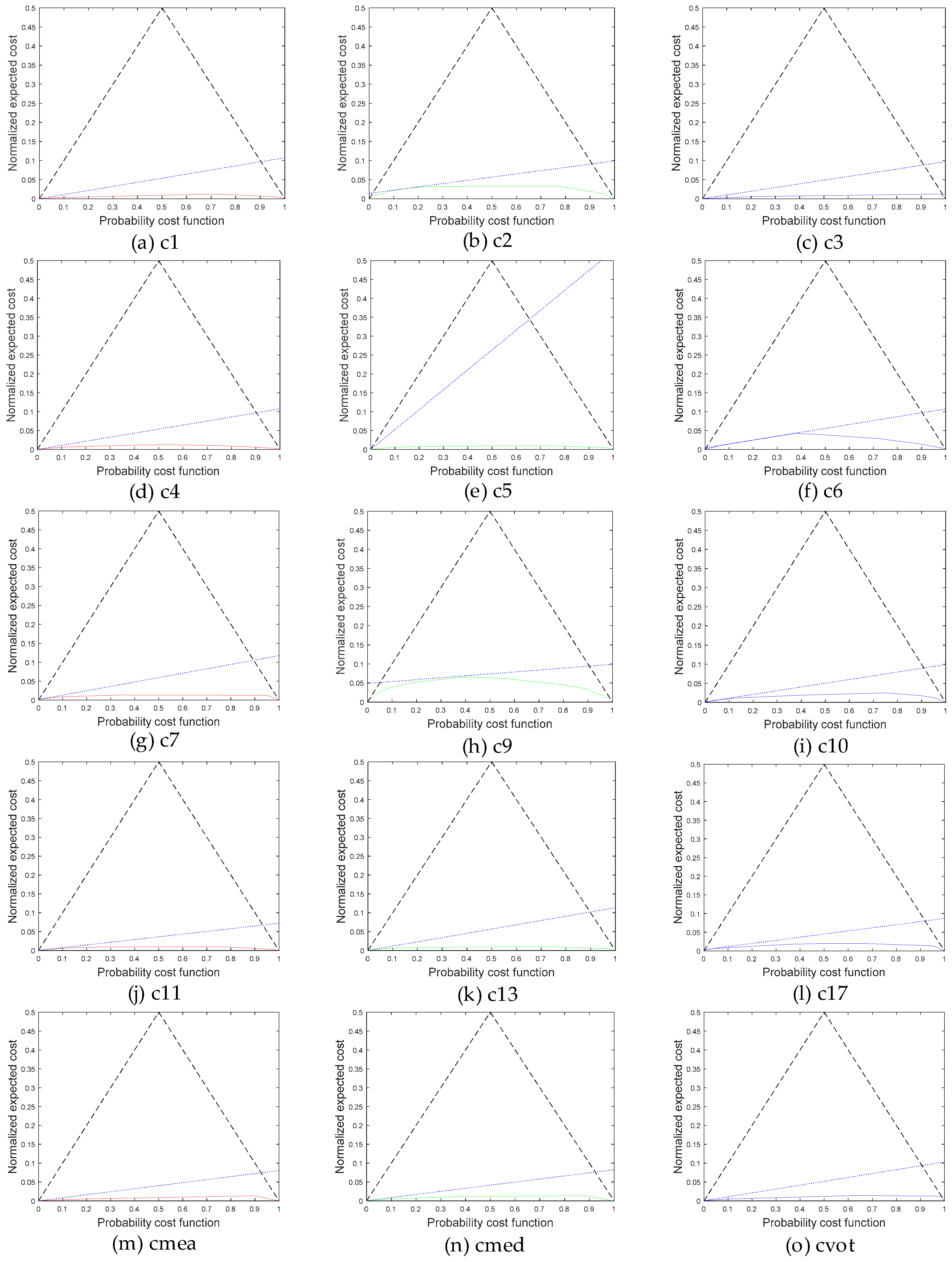
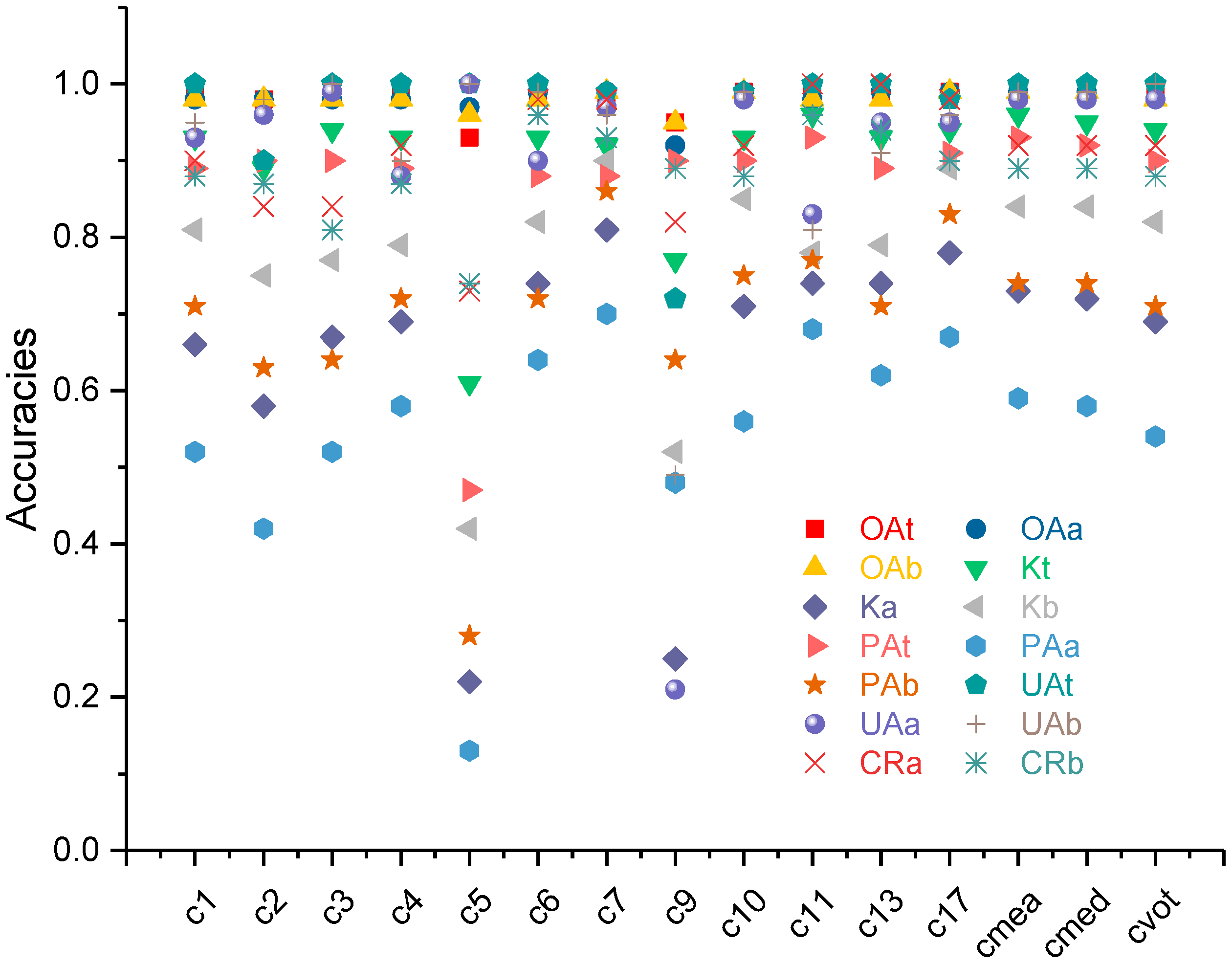
3.2. Measuring Performance

Performance evaluation is crucial in the assessment of a set of SCDDs. For Table 3, the false negative rate (FNR) gives the error on the positive class, while the false positive rate (FPR) shows the error on the negative class. Meanwhile, P is precision, and R denotes recall equivalent with TPR. The statistical metrics can be grouped into (1) a group that the smaller is the better, i.e., the FNR and FPR, and (2) another group that the greater is the better, i.e., P, R, F1, and AUC. Although it is difficult to describe all SCDDs together, we attempt to make it possible by rating them on a rank table later. Table 3 illustrates that the FNR (e.g., the c5) and FPR (e.g., the c2 and c9) are prominently higher than two known inferior SCDDs (e.g., the c5 and c9), and a slightly inferior one (e.g., c2) is marked as well. Additionally, these unqualified SCDDs are again attention-catching in the second group. For all SCDDs, the precision (e.g., the c2 and c9), recall (e.g., the c5), and F1 score (e.g., the c2, c5, and c9) support the analysis drawn from the first group, while the AUC error always appears mediocre. However, there are some differences owing to the measuring ability of statistical metrics and the intrinsic characteristics of the diverse SCDDs. The ROC curve (see Figure 8) gives a two-dimensional depiction of the performance of the SCDD. This is due to too many SCDDs with the approximate accuracies so that discriminating the individual ROC curve seems difficult. Thus, we plot them one by one, and the aforementioned inferior SCDDs still can be well reflected. Note that the c5 has the lowest operation point, while the c2 and c9 are found in terms of the ROC curve. In addition, the c6 deserves attention. Here, the ROC graphs are not going to be read significantly, as the purpose is achieved. The cost curve (see Figure 9) is a specific performance visualizer using the expected cost, another technique to measure the performance of SCDDs. Each operating point appears as a line in this plot, while the certain one of them is indicated by the dotted line. The combination of operating points that forms the lower hull is indicated by the thick curve and shows the best operating points over the range of costs. Here, the dotted line of c5, and the thick arcs of c2 and c9, again support the performance analysis drawn from the Figure 8. In particular, c6 has a representation that is the same as the ROC graph.
The confusion matrix is often applied to visualize the performance of the SCDD by a specific table layout. The OA means overall accuracy, K is the Kappa coefficient, PA denotes the producer’s accuracy, and UA represents the user’s accuracy. It is somewhat intricate that we structure two kinds of confusion matrices together (see Figure 10), which look similar but not identical. That is the reason why we design two types of confusion matrix (1) classifier-dependent (i.e., OAt, Kt, PAt, and UAt), which is generated using the test set; and (2) classifier-independent (i.e., OAa, Ka, PAa, UAa, OAb, Kb, PAb, and UAb), which is produced by utilizing the reference result for “sa” and “sb”. For the two classifier-independent error matrices, which give an analogous presentation and a comforting result, though with a slight discrepancy in the amplitude, the inferior SCDDs, i.e., the c5 has a smaller K and PA while the c9 has a smaller K and UA. As for the classifier-dependent confusion matrix, all SCDDs have good performance except for the c5 has a lower K and PA while the c9 has a lower K and UA.
The summary can be drawn as (1) overall accuracy appears mediocre or fails in the face of the SCDD for the imbalanced data; and (2) two classifier-independent error matrices demonstrate that the SCDDs are, indeed, fixed by unchangeable splitting samples. Meanwhile, they seem worse and more unstable compared to the classifier-dependent matrices, which may be disturbed in the presence of more uncertainty. The correct rate (see Figure 10, and Table 4) is a custom performance measure, which is used for validation. Here, the true labels used are a subset of the positive samples drawn from a merged set for the “sa” and “sb”. This measure is a simple attempt to repeat and verify the previous analysis.

4. Discussion

4.1. Selection Criteria
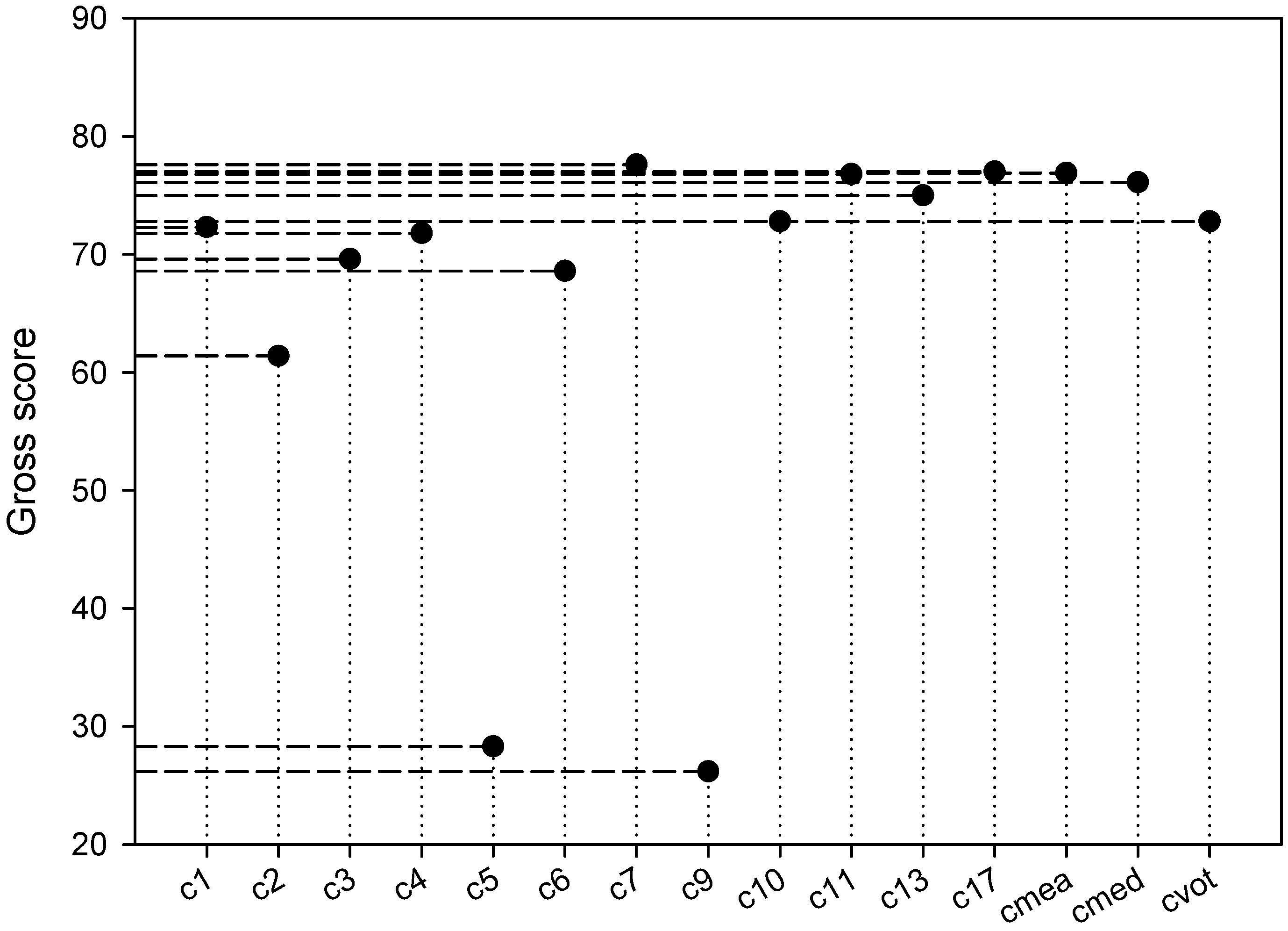
Although sufficient statistical analyses have been conducted, it is not known how to recognize which SCDD looks good. In fact, it is not easy to determine which is a fine, or even the best in the face of so many SCDDs with multiple performance measures. Therefore, we want to set up a handful of naive selection criteria to achieve such a goal by means of a rank board (see Table 4). For this work, more empirical selection criteria are adopted. Intrinsically, most of the statistical metrics are derived from the basic errors (i.e., the true positive, the true negative, the false positive, and the false negative). The derived measures (i.e., the precision, recall, F1, AUC, OA, KC, PA, and UA) could be quantitatively analyzed with actions such as rating and scoring. Note that the AUC measure appears mediocre herein. The OA may not be a reliable metric for the real performance of the SCDD in this study, because it yields misleading results supposing the training data are imbalanced when the numbers of observations in different classes vary greatly. The ROC curve and cost graph are used for supporting numerical indicators, which are especially suitable for classification problems in which there are only two classes (i.e., the positive and negative classes). The limitation [70] of both ROC analysis and cost curve is the lack of any effective method to show the performance results obtained from several different data sets in a single plot. This difficulty follows the fact that only two dimensions are used to present the performance of a single data set.
It is important to realize the optimal selection criteria for the hybrid classifiers, such as comparing the performance of an ensemble classifier with a member classifier, which is also presented in this study. The fixed combination strategies or so-called rules (i.e., the mean rule, median rule, and voting rule), are more likely to obtain better classification results, just as the inferior classifiers will reduce the whole performance. In particular, the time taken will be an insufferable problem. It is crucial to address the question of under what criteria does one classifier outperform another. Additionally, a decision needs to be made to determine which classifier should be selected over others. That is if, given the current operating conditions, a set of selection criteria can be derived. It is often easy, by varying the parameter setting, such as a threshold or the variables of the mathematical model, or by varying the class distribution in the training set, to create a whole set of SCDDs. One commonly used selection criterion is to select the SCDD whose parameter settings and training conditions most closely agree with the current operating conditions, which is called the performance-independent criterion [75]. This is the reason why we try to fix all irrelevant conditions prior to developing the performance-dependent selection criteria. A plain criterion is to choose the qualified SCDDs regardless of their training conditions or parameter settings.

4.2. Scoring Model

For SCDDs with multiple performance measures, it would be expected for them to be scored. Then, there is always one possibility that all SCDDs can be quantitatively evaluated and scored. Consequently, a score-oriented method is presented here to clarify this concern. In this study, we put forward a kind of scoreboard on the basis of the rank board to give each SCDD an explicit score so that we can determine which SCDD is optimal.
According to Table 5, we use the rows (M.) to denote the measures and the columns (C.) to represent the different SCDDs. Signs are used to identify the metric belonging to which group: “–” denotes the error metric (i.e., the smaller the better), while “+” is the accuracy metric (i.e., the greater the better). The score variable Scj is calculated by the following equation:
s i j ( x ) = { n x i j Min ( x i ) ( Max ( x i ) Min ( x i ) ) / n   if   sign = x i j Min ( x i ) ( Max ( x i ) Min ( x i ) ) / n    if   sign = + ,
or
s i j ( x ) = { Max ( x i ) x i j ( Max ( x i ) Min ( x i ) ) / n   if   sign = n Max ( x i ) x i j ( Max ( x i ) Min ( x i ) ) / n   if   sign = + ,
and
S c j = s j ,
where xi represents the measures in the ith row, xj represents SCDDs in the jth column, and xij denotes the measured value of the jth SCDD with ith metric. The si represents the scores in the ith row, the sj represents the scores in the jth column, and the sij denotes the score value of the jth SCDD with the ith metric. Scj represents the total score of the jth SCDD. For simplicity, we assume that there are five SCDDs and five measures herein to facilitate the illustration of the scoreboard and the derivation of Equations (2)–(4). The n is a key scale to slice a certain metric for all SCDDs so that each SCDD can be assigned a normalized float value (ranging from 0 to n) associated with this metric. In the end, the gross score of every SCDD can be obtained and plotted by performing the summation by column. Figure 11 illustrates that two inferior SCDDs, i.e., the c5 is underestimated, and the c9 is overestimated, which are prominently identified. Meanwhile, two slightly inferior SCDDs, i.e., the c2 and c6, are apt to be observed again.

4.3. McNemar’s Test

The four-cell confusion matrix is very intuitive to show the similarities and differences between the proportions (i.e., the true and false allocated parts) concerning two sets of specific labels. On the basis of the error table, we wish to achieve the statistical significance of the differences between the proportions using McNemar’s test [76] so as to assess two allocated results, which are obtained by two SCDDs, or just given, under a position-specific comparison. Here, McNemar’s test is specifically useful for comparing paired proportions derived from two sets of samples. In the formulas below, we use the notations:
p d i s c = p F + + p F p d i f f = p F + p F ,
where the p F + is the proportion of testing samples that the first SCDD is true, and the second is false; meanwhile, the p F denotes the proportion of testing samples that the first SCDD is false while the second is true. Thus, McNemar’s test focuses on the proportions of testing samples that one SCDD is true while another is false (and vice versa) [41].
S E p = ( p d i s c p d i f f 2 ) / N ,
where SEp represents the standard error derived from the difference between the proportions, and N is the total number of the pairs of objects. McNemar’s test will perform the evaluation of the 100 ( 1 α ) % confidence interval for comparing the difference between two accuracy values based on the differences ( D α ) between the proportions. Assuming a normal distribution z α , the general expression of the confidence interval [76] can be expressed as:
D a ± z α S E p .
For exploring in a straightforward manner, we split Equation (7) into a real image, then the image part may be more crucial to give the proper assessment with regard to a confusion matrix. In this way, the statistical assessment of the differences is carried out to determine if these are significantly different or not [76]. Since three kinds of error matrices are presented in this study, here we name them as CDt (i.e., the classifier-dependent using the test set), CIa (i.e., the classifier-independent using the reference map of the “sa”), and CIb (i.e., the classifier-independent using the reference map of the “sb“).
The difference between the accuracies yielded by the paired SCDDs (or two sets of labels) is D α , ranging from D a | z α | S E p to D a + | z α | S E p at the 100 × (1 − 0.05)% confidence interval. In order to make all confidence intervals comparable, the one-sided absolute range ( | z α | S E p ) around D a is exhibited in Table 6. Two inferior SCDDs (i.e., the c5 and c9) have their appearances again. As for two slightly inferior SCDDs (i.e., the c2 and c6), only the c2 can be observed. Such results estimated by McNemar’s test provide a useful back-up to previous analysis.

4.4. Special Concerns and Limitations

Panax notoginseng is a rare kind of ginseng, and which also is an antique and endangered medicinal plant (i.e., a traditional Chinese geoherb). This paper aims to explore its potential and provides some insights into the application of SCDDs for the landscape-scale mapping of Panax notoginseng. We wish this work could be the referenced technical basis for exploring more novel points that make outstanding contributions and provide the fruitful information for studies on the quality assurance of the production of TCM, precision farming, the construction of agro-ecosystems, sustainable development, and the protection of biodiversity of Panax notoginseng. Special concerns and limitations of this study can be summarized as follows:
This work utilizes a manually-collected set of samples of the target class and grid-constraint uniformly-collected negative samples. The uncertainty exists that a few possible land-cover classes may be left out, even though the classification results look rather good.
Thirteen SCDDs are employed and compared, however, there may be many other algorithms and their variants. Anyhow, the available ones have been used in this study.
The comparison with the different SCDDs does not judge them to be good or not. Actually, we wish to extend the ability of SCDDs to achieve the expected experiences in a straightforward way to find the optimal approach to monitoring the plant pattern changes of Panax notoginseng.
The class imbalance is a non-negligible problem in terms of a real specific land-cover classification using SCDDs. We strive for trying to observe what influences it would cause, and find two mediocre-appearing measures, i.e., the OA and AUC.
The selection criteria and scoring model are presented to determine the optimal SCDD which is outstanding and deserves attention.
The division of the site-specific error matrices by discriminating if the SCDD is dependent on the training set or not provides a more comprehensive approach to assess the final results.
The combination of SCDDs which are taken as the base classifiers can reduce the error or improve the accuracy. However, lower computational efficiency would be an annoying problem. Additionally, the pruned ensembles can give better performance.
Some classification accuracies may not be the reliable indicators, particularly if the training data are imbalanced [41,77]. As single-class data description is a special type of one-class classification, there are difficulties that may exist when trying to fit a single-class learner using the positive samples only. If SCDDs are trained with the samples of the single target class, then only the sensitivity can be estimated. There is a possibility that using only the sensitivity to fine-tune an algorithm may result in a class descriptor with high sensitivity but low specificity and overestimating the true extension of the class of interest [41]. In terms of the scope of this study, the introduction of single-class data description regarding remote-sensing mapping of Panax notoginseng fields based on P-learning, which provides us the new insights to promote the development of the resource inventory and dynamic monitoring of Panax notoginseng.

5. Conclusions

Natural TCM resources have seldom been observed and monitored from space before. Due to the promoted GAP technique, the small or fragmented parcels covered by black plastic sheets create the opportunity and probability for us to recognize and analyze the eco-geographic characteristics of Panax notoginseng at a landscape-scale. This paper delineates an application whereby a stack of SCDDs is used for remote-sensing mapping of Panax notoginseng fields through P-learning. The measuring performance of SCDDs provides us the challenging insights to define the selection criteria and scoring proof for choosing an optimal SCDD for remote-sensing mapping a specific landscape class. Future work would involve (1) developing new algorithms to enrich the approaches of specific land cover mapping; (2) improving the design sets, updating the sampling strategy, and overcoming the imbalance issue; and (3) extending to the state-of-the-art SCDDs published, which have not been presented in this study.

Author Contributions

F.D. and S.P. conceived and designed the experiments; S.P. performed the experiments and analyzed the data; and all relevant co-authors participated in writing and editing the paper.

Funding

Research Fund of State Key Laboratory of Geohazard Prevention and Geoenvironment Protection (SKLGP2018Z006).

Acknowledgments

The authors thank the editors and the anonymous reviewers for their insightful comments and helpful suggestions, which highly improved the quality of the manuscript. We are grateful to D. Tax for the development and free use of the dd_tools.

Conflicts of Interest

The authors declare no conflict of interest. The funders had no role in the design of the study; in the collection, analyses, or interpretation of data; in the writing of the manuscript, and in the decision to publish the results.

References

  1. Tsai, C. A brief introduction to traditional Chinese medicine. In 30 Years’ Review of China’s Science and Technology; World Scientific: Singapore, 1981; pp. 125–138. [Google Scholar]
  2. Li, X.; Yang, G.; Li, X.; Zhang, Y.; Yang, J.; Chang, J.; Sun, X.; Zhou, X.; Guo, Y.; Xu, Y.; et al. Traditional Chinese medicine in cancer care: A review of controlled clinical studies published in Chinese. PLoS ONE 2013, 8, e60338. [Google Scholar]
  3. Stone, R. Lifting the veil on traditional Chinese medicine. Science 2008, 319, 709–710. [Google Scholar] [CrossRef] [PubMed]
  4. Xiong, X. Integrating traditional Chinese medicine into Western cardiovascular medicine: An evidence-based approach. Nat. Rev. Cardiol. 2015, 12, 374. [Google Scholar] [CrossRef] [PubMed]
  5. Harvey, A.L.; Edrada-Ebel, R.; Quinn, R.J. The re-emergence of natural products for drug discovery in the genomics era. Nat. Rev. Drug Discov. 2015, 14, 111–129. [Google Scholar] [CrossRef] [PubMed] [Green Version]
  6. Dong, J. The relationship between traditional Chinese medicine and modern medicine. Evid.-Based Complement. Altern. 2013, 2013, 153148. [Google Scholar] [CrossRef] [PubMed]
  7. Xue, T.; Roy, R. Studying traditional Chinese medicine. Science 2003, 300, 740–741. [Google Scholar] [CrossRef] [PubMed]
  8. General Administration of Quality Supervision, Inspection and Quarantine of the People’s Republic of China. Provisions for the Protection of Products of Geographical Indication. Available online: http://www.wipo.int/edocs/lexdocs/laws/en/cn/cn041en.pdf (accessed on 10 August 2018).
  9. Addor, F.; Grazioli, A. Geographical indications beyond wines and spirits. J. World Intellect. Prop. 2002, 5, 865–897. [Google Scholar] [CrossRef]
  10. Standing Committee of the National People’s Congress. Law of the People’s Republic of China on Traditional Chinese Medicine. Available online: http://www.gov.cn/xinwen/2016-12/26/content_5152773.htm (accessed on 10 August 2018).
  11. Fan, Z.; Miao, C.; Qiao, X.; Zheng, Y.; Chen, H.; Chen, Y.; Xu, L.; Zhao, L.; Guan, H. Diversity, distribution, and antagonistic activities of rhizobacteria of Panax notoginseng. J. Ginseng Res. 2016, 40, 97–104. [Google Scholar] [CrossRef] [PubMed]
  12. Park, H.J.; Kim, D.H.; Park, S.J.; Kim, J.M.; Ryu, J.H. Ginseng in traditional herbal prescriptions. J. Ginseng Res. 2012, 36, 225–241. [Google Scholar] [CrossRef] [PubMed]
  13. Wei, J.X.; Du, Y.C. Modern Science Research and Application of Panax Notoginseng; Yunnan Science and Technology Press: Kunming, China, 1996. [Google Scholar]
  14. Zhou, Y.Q.; Chen, S.L.; Zhang, B.G.; Zhang, J.S.; Zhang, J.; Chen, Z.J.; Cun, X.M. Studies on the resources survey methods of Panax notogingseng based on remote sensing. China J. Chin. Mater. Med. 2005, 30, 1902–1905. [Google Scholar]
  15. The State Council of the People’s Republic of China. Several Opinions of the State Council on Supporting and Promoting the Development of Traditional Chinese Medicine. Available online: http://www.gov.cn/zwgk/2009-05/07/content_1307145.htm (accessed on 10 August 2018).
  16. The State Council Information Office of the Peoples Republic of China. Health Service Development Plan of Traditional Chinese Medicine (2015–2020). Available online: http://www.gov.cn/zhengce/ content/2015-05/07/content_9704.htm (accessed on 10 August 2018).
  17. The Ministry of Science and Technology of the People’s Republic of China. Outline of Traditional Chinese Medicine Innovation and Development Plan (2006–2020). Available online: http://www.most.gov.cn/tztg/200703/t20070320_42240.htm (accessed on 10 August 2018).
  18. Sun, X.; Lin, D.; Wu, W.; Lv, Z. Translational Chinese medicine: A way for development of traditional Chinese medicine. Chin. Med. 2011, 2, 186–190. [Google Scholar] [CrossRef]
  19. Sanchez-Hernandez, C.; Boyd, D.S.; Foody, G.M. One-class classification for mapping a specific land-cover class: SVDD classification of fenland. IEEE Trans. Geosci. Remote Sens. 2007, 45, 1061–1073. [Google Scholar] [CrossRef]
  20. Boyd, D.S.; Foody, G.M. Changing Land Cover; Global Environmental Issues; John Wiley & Sons: Hoboken, NJ, USA, 2004; pp. 65–94. [Google Scholar]
  21. Cihlar, J. Land cover mapping of large areas from satellites: Status and research priorities. Int. J. Remote Sens. 2000, 21, 1093–1114. [Google Scholar] [CrossRef] [Green Version]
  22. Wang, J.; Xiao, X.; Qin, Y.; Dong, J.; Zhang, G.; Kou, W.; Jin, C.; Zhou, Y.; Zhang, Y. Mapping paddy rice planting area in wheat-rice double-cropped areas through integration of Landsat-8 OLI, MODIS, and PALSAR images. Sci. Rep. 2015, 5, 10088. [Google Scholar] [CrossRef] [PubMed]
  23. Thenkabail, P.S.; Knox, J.W.; Ozdogan, M.; Gumma, M.K.; Congalton, R.G.; Wu, Z.; Milesi, C.; Finkral, A.; Marshall, M.; Mariotto, I.; et al. Assessing future risks to agricultural productivity, water resources and food security: How can remote sensing help? Photogramm. Eng. Rem. Sens. 2012, 78, 773–782. [Google Scholar]
  24. Foody, G.M.; Mathur, A.; Sanchez-Hernandez, C.; Boyd, D.S. Training set size requirements for the classification of a specific class. Remote Sens. Environ. 2006, 104, 1–14. [Google Scholar] [CrossRef]
  25. Song, B.; Li, P.; Li, J.; Plaza, A. One-class classification of remote sensing images using kernel sparse representation. IEEE J-STARS 2016, 9, 1613–1623. [Google Scholar] [CrossRef]
  26. Chen, C.H. An overview of recent progress on information processing for remote sensing. In Information Processing for Remote Sensing; World Scientific: Singapore, 1999; pp. 39–49. [Google Scholar]
  27. Foody, G.M. Status of land cover classification accuracy assessment. Remote Sens. Environ. 2002, 80, 185–201. [Google Scholar] [CrossRef]
  28. Wilkinson, G.G. Results and implications of a study of fifteen years of satellite image classification experiments. IEEE Trans. Geosci. Remote Sens. 2005, 43, 433–440. [Google Scholar] [CrossRef]
  29. Chen, C.H. Frontiers of Remote Sensing Information Processing; World Scientific: Singapore, 2003. [Google Scholar]
  30. Cristianini, N.; Shawe-Taylor, J. An Introduction to Support Vector Machines and Other Kernel-Based Learning Methods; Cambridge University Press: Cambridge, UK, 2000. [Google Scholar]
  31. Wan, B.; Guo, Q.; Fang, F.; Su, Y.; Wang, R. Mapping US urban extents from MODIS data using one-class classification method. Remote Sens. 2015, 7, 10143–10163. [Google Scholar] [CrossRef]
  32. Mathieu, P.P.; Aubrecht, C. Earth Observation Open Science and Innovation; Springer Open: Cham, Switzerland, 2018; pp. 165–218. [Google Scholar]
  33. Tse, C.H.; Lam, E.Y. Geological applications of machine learning on hyperspectral remote sensing data. Proc. SPIE Int. Soc. Opt. Eng. 2015, 9405, 940512. [Google Scholar]
  34. Brown, M.E.; Lary, D.J.; Vrieling, A.; Stathakis, D.; Mussa, H. Neural networks as a tool for constructing continuous NDVI time series from AVHRR and MODIS. Int. J. Remote Sens. 2008, 29, 7141–7158. [Google Scholar] [CrossRef] [Green Version]
  35. Lary, D.J.; Remer, L.A.; MacNeill, D.; Roscoe, B.; Paradise, S. Machine Learning and Bias Correction of MODIS Aerosol Optical Depth. IEEE Geosci. Remote Sens. Lett. 2009, 6, 694–698. [Google Scholar] [CrossRef]
  36. Aurin, D.A.; Mannino, A. A Database for Developing Global Ocean Color Algorithms for Colored Dissolved Organic Material, CDOM Spectral Slope, and Dissolved Organic Carbon. In Proceedings of the Ocean Optics XXI, Glasgow, Scotland, UK, 8–12 October 2012. [Google Scholar]
  37. Lary, D.J.; Alavi, A.H.; Gandomi, A.H.; Walker, A.L. Machine learning in geosciences and remote sensing. Geosci. Front. 2016, 7, 3–10. [Google Scholar] [CrossRef]
  38. Khobragade, A.N.; Raghuwanshi, M.M. Contextual Soft Classification Approaches for Crops Identification Using Multi-sensory Remote Sensing Data: Machine Learning Perspective for Satellite Images; Springer International Publishing: Cham, Switzerland, 2015; pp. 333–346. [Google Scholar]
  39. FAO. Development of a Framework for Good Agricultural Practices. Available online: http://www.fao.org/docrep/meeting/006/y8704e.htm (accessed on 10 August 2018).
  40. Davis, N. Controlled-environment agriculture-past, present and future. Food Technol. 1985, 39, 124–126. [Google Scholar]
  41. Silva, J.; Bacao, F.; Caetano, M. Specific Land Cover Class Mapping by Semi-Supervised Weighted Support Vector Machines. Remote Sens. 2017, 9, 181. [Google Scholar] [CrossRef]
  42. Mack, B.; Roscher, R.; Stenzel, S.; Feilhauer, H.; Schmidtlein, S.; Waske, B. Mapping raised bogs with an iterative one-class classification approach. ISPRS J. Photogramm. 2016, 120, 53–64. [Google Scholar] [CrossRef]
  43. Liu, X.; Liu, H.; Gong, H.; Lin, Z.; Lv, S. Appling the one-class classification method of maxent to detect an invasive plant Spartina alterniflora with time-series analysis. Remote Sens. 2017, 9, 1120. [Google Scholar] [CrossRef]
  44. Marconcini, M.; Fernández-Prieto, D.; Buchholz, T. Targeted land-cover classification. IEEE Trans. Geosci. Remote Sens. 2014, 52, 4173–4193. [Google Scholar] [CrossRef]
  45. Sahare, M.; Gupta, H. A review of multi-class classification for imbalanced data. Int. J. Adv. Comput. Res. 2012, 2, 160–164. [Google Scholar]
  46. Sun, Y.; Wong, A.K.C.; Kamel, M.S. Classification of imbalanced data: A review. Int. J. Pattern Recogn. Artif. Intell. 2009, 23, 687–719. [Google Scholar] [CrossRef]
  47. Tax, D.M.J. One-Class Classification: Concept-Learning in the Absence of Counter-Examples. Ph.D. Thesis, Delft University of Technology, Delft, The Netherlands, 2001; p. 65. [Google Scholar]
  48. Khan, S.S.; Madden, M.G. One-class classification: Taxonomy of study and review of techniques. Knowl. Eng. Rev. 2014, 29, 345–374. [Google Scholar] [CrossRef]
  49. Normile, D. The new face of traditional Chinese medicine. Science 2003, 299, 188–190. [Google Scholar] [CrossRef] [PubMed]
  50. Chen, L.; Dong, K.; Yang, Z.; Dong, Y.; Tang, L.; Zheng, Y. Allelopathy autotoxcity effect of successive cropping obstacle and its alleviate mechanism by intercropping. Chin. Agric. Sci. Bull. 2017, 33, 91–98. [Google Scholar]
  51. Fu, G.; Zhang, Q.; Liang, C.; Cheng, Z. Stereoscopic planting pattern of kernel-used apricot and medicinal plants in the loess drought hilly region in West Henan Province. Med. Plant 2011, 2, 5–11. [Google Scholar]
  52. Panigrahy, S.; Sharma, S.A. Mapping of crop rotation using multidate Indian remote rensing satellite digital data. ISPRS J. Photogramm. 1997, 52, 85–91. [Google Scholar] [CrossRef]
  53. Pirkouhi, M.G.; Nobahar, A.; Dadashi, M.A. Effects of variety, planting pattern and density of plant phenology traits basil plants (Ocimum basilicum L.). Int. J. Agric. Crop Sci. 2012, 4, 1221–1227. [Google Scholar]
  54. Yunusa, I.A.M. Effects of planting density and plant arrangement pattern on growth and yields of maize (Zea mays L.) and soya bean (Glycine max (L.) Merr.) grown in mixtures. J. Agric. Sci. 1989, 112, 1–8. [Google Scholar] [CrossRef]
  55. Song, C.; Woodcock, C.E.; Seto, K.C.; Lenney, M.P.; Macomber, S.A. Classification and change detection using Landsat TM data: When and how to correct atmospheric effects? Remote Sens. Environ. 2001, 75, 230–244. [Google Scholar] [CrossRef]
  56. Yang, D.; Chen, J.; Zhou, Y.; Chen, X.; Chen, X.; Cao, X. Mapping plastic greenhouse with medium spatial resolution satellite data: Development of a new spectral index. ISPRS J. Photogramm. 2017, 128, 47–60. [Google Scholar] [CrossRef]
  57. Von Elsner, B.; Briassoulis, D.; Waaijenberg, D.; Mistriotis, A.; Von Zabeltitz, C.; Gratraud, J.; Russo, G.; Suay-Cortes, R. Review of structural and functional characteristics of greenhouses in European Union countries: Part I, design requirements. J. Agric. Eng. Res. 2000, 75, 1–16. [Google Scholar] [CrossRef]
  58. Foody, G.M.; Boyd, D.S.; Sanchez-Hernandez, C. Mapping a specific class with an ensemble of classifiers. Int. J. Remote Sens. 2007, 28, 1733–1746. [Google Scholar] [CrossRef]
  59. Mack, B.; Roscher, R.; Waske, B. Can I trust my one-class classification? Remote Sens. 2014, 6, 8779–8802. [Google Scholar] [CrossRef]
  60. McLachlan, G.; Peel, D. Finite Mixture Models; John Wiley & Sons: Hoboken, NJ, USA, 2004. [Google Scholar]
  61. Møller, M.F. A scaled conjugate gradient algorithm for fast supervised learning. Neural Netw. 1993, 6, 525–533. [Google Scholar] [CrossRef]
  62. Arthur, D.; Vassilvitskii, S. In k-means++: The advantages of careful seeding. In Proceedings of the Eighteenth Annual ACM-SIAM Symposium on Discrete Algorithms, New Orleans, LA, USA, 7–9 January 2007; pp. 1027–1035. [Google Scholar]
  63. Kohonen, T. The self-organizing map. Neurocomputing 1998, 21, 1–6. [Google Scholar] [CrossRef]
  64. Gallager, R.G.; Humblet, P.A.; Spira, P.M. A distributed algorithm for minimum-weight spanning trees. ACM Trans. Program. Lang. Syst. (TOPLAS) 1983, 5, 66–77. [Google Scholar] [CrossRef]
  65. Altman, N.S. An introduction to kernel and nearest-neighbor nonparametric regression. Am. Stat. 1992, 46, 175–185. [Google Scholar]
  66. Tax, D.; Ypma, A.; Duin, R. Support vector data description applied to machine vibration analysis. In Proceedings of the 5th Annual Conference of the Advanced School for Computing and Imaging, Heijen, The Netherlands, 15–17 June 1999; pp. 15–23. [Google Scholar]
  67. Parzen, E. On estimation of a probability density function and mode. Ann. Math. Stat. 1962, 33, 1065–1076. [Google Scholar] [CrossRef]
  68. Jolliffe, I.T. Principal component analysis and factor analysis. In Principal Component Analysis; Springer: New York, NY, USA, 2002; pp. 150–166. [Google Scholar]
  69. Powers, D.M. Evaluation: From precision, recall and F-measure to ROC, informedness, markedness and correlation. J. Mach. Learn. Technol. 2011, 2, 37–63. [Google Scholar]
  70. Fawcett, T. An introduction to ROC analysis. Pattern Recogn. Lett. 2006, 27, 861–874. [Google Scholar] [CrossRef]
  71. Bradley, A.P. The use of the area under the ROC curve in the evaluation of machine learning algorithms. Pattern Recogn. 1997, 30, 1145–1159. [Google Scholar] [CrossRef] [Green Version]
  72. Hanley, J.A.; McNeil, B.J. The meaning and use of the area under a receiver operating characteristic (ROC) curve. Radiology 1982, 143, 29–36. [Google Scholar] [CrossRef] [PubMed]
  73. Drummond, C.; Holte, R.C. Explicitly representing expected cost: An alternative to ROC representation. In Proceedings of the 6th ACM SIGKDD International Conference on Knowledge Discovery and Data Mining, Boston, MA, USA, 20–23 August 2000; pp. 198–207. [Google Scholar]
  74. Stehman, S.V. Selecting and interpreting measures of thematic classification accuracy. Remote Sens. Environ. 1997, 62, 77–89. [Google Scholar] [CrossRef]
  75. Ting, K.M. Matching model versus single model: A study of the requirement to match class distribution using decision trees. In European Conference on Machine Learning; Springer: Berlin/Heidelberg, Germany, 2004; pp. 429–440. [Google Scholar]
  76. Foody, G.M. Classification accuracy comparison: Hypothesis tests and the use of confidence intervals in evaluations of difference, equivalence and non-inferiority. Remote Sens. Environ. 2009, 113, 1658–1663. [Google Scholar] [CrossRef] [Green Version]
  77. Hwang, J.P. A new weighted approach to imbalanced data classification problem via support vector machine with quadratic cost function. Expert Syst. Appl. 2011, 38, 8580–8585. [Google Scholar] [CrossRef]
Figure 1. Panax notoginseng is a well-known geoherb, which has acquired a very favorable reputation for the treatment of blood disorders, including blood stasis, bleeding, and blood deficiency. Its root can be turned to powder as a medicinal material, and the shadenet cover can be observed from space by means of satellite imagery.
Applsci 08 01448 g001
Figure 2. Study area in Wenshan City, Wenshan Prefecture, Yunnan Province, China.
Applsci 08 01448 g002
Figure 3. Shade house. Sub-figures are the snapshots and photos in the different phases of the construction of a shade house of Panax notoginseng including the materials for building, i.e., sticks (5 cm × 2 m), upright rods, and black plastic net over the poles; viewpoints for the observation, i.e., parallel to bed, perpendicular to bed, at close range, over a long distance, and from a satellite image.
Applsci 08 01448 g003
Figure 4. Sampling sites. (a) The site #45; (b) the sites in Wenshan City.
Applsci 08 01448 g004
Figure 5. Reference results. (a) a regular subset, (b) the overlap, (c) an irregular subset of Landsat-8 OLI image, and (d) the reference result for the “sa”; (e) a regular subset, (f) the overlap, (g) an irregular subset of Landsat-8 OLI image, and (h) the reference result for the “sb”.
Applsci 08 01448 g005
Figure 6. Classification results which are shown in false-color style in comparison with the reference result for the “sa”. (a) Reference result; (b) simple Gaussian target distribution (SGTD); (c) robust Gaussian target distribution (RGTD); (d) minimum covariance determinant Gaussian (MCDG); (e) mixture of Gaussian (MoG); (f) Parzen density estimator (PDE); (g) auto-encoder neural network (AENN); (h) k-means; (i) principal component analysis (PCA); (j) self-organizing map (SOM); (k) minimum spanning tree (MST); (l) k-nearest neighbor (K-NN); (m) incremental support vector data description (IncSVDD); (n) mean combiner (meanc); (o) median combiner (medianc); and (p) voting combiner (votec). Here, the white pixels means the well estimated, the magenta means underestimated, and the green means overestimated.
Applsci 08 01448 g006
Figure 7. Classification results which are shown in false-color style in comparison with the reference result for the “sb”. (a) Reference result; (b) SGTD; (c) RGTD; (d) MCDG; (e) MoG; (f) PDE; (g) AENN; (h) k-means; (i) PCA; (j) SOM; (k) MST; (l) K-NN; (m) IncSVDD; (n) meanc; (o) medianc; and (p) votec.
Applsci 08 01448 g007
Figure 8. ROC curves. (a) c1: SGTD; (b) c2: RGTD; (c) c3: MCDG; (d) c4: MoG; (e) c5: PDE; (f) c6: AENN; (g) c7: k-means; (h) c9: PCA; (i) c10: SOM; (j) c11: MST; (k) c13: K-NN; (l) c17: IncSVDD; (m) cmea: meanc; (n) cmed: medianc; and (o) cvot: votec.
Applsci 08 01448 g008
Figure 9. Cost curves. (a) c1: SGTD; (b) c2: RGTD; (c) c3: MCDG; (d) c4: MoG; (e) c5: PDE; (f) c6: AENN; (g) c7: k-means; (h) c9: PCA; (i) c10: SOM; (j) c11: MST; (k) c13: K-NN; (l) c17: IncSVDD; (m) cmea: meanc; (n) cmed: medianc; and (o) cvot: votec.
Applsci 08 01448 g009
Figure 10. Accuracy metrics derived from the confusion matrix. Here, the postfix “t” means taking the test set as the true labels, while the “a” and “b” mean taking the reference results as the true labels, respectively. The CRa and CRb are the correct rates of the classification results in comparison with the true labels for the “sa” and “sb”.
Applsci 08 01448 g010
Figure 11. Scoring result, n = 4.
Applsci 08 01448 g011
Table 1. Cloud cover statistics of a 16-day revisited Landsat-8 OLI scene (path/row 128/044) until May 2017.
Cloud (%)NumberPercentages
0–1033.41
10–2077.95
20–401314.77
40–601719.32
60–802326.14
80–1002528.41
Table 2. Binary error matrix.
TypesPredicted Label
TargetOther
Actual LabelTargettrue positive (TP)false positive (FP)
Otherfalse negative (FN)true negative (TN)
Table 3. Accuracy metrics, i.e., the FNR, FPR, P, R, F1, and AUC.
c1c2c3c4c5c6c7c9c10c11c13c17CmeaCmedCvot
FNR0.110.100.100.110.530.120.120.100.100.070.110.090.070.080.10
FPR0.000.010.000.000.000.000.000.050.000.000.000.000.000.000.00
P1.000.901.001.001.001.000.990.720.991.001.000.981.001.001.00
R0.890.900.900.890.470.880.880.900.900.930.890.910.930.920.90
F10.940.900.950.940.640.940.930.800.940.960.940.940.960.960.95
AUC1.000.990.991.001.001.001.000.981.001.001.001.001.001.000.99
Table 4. Rank table. Here, the FN and FP are the false negative rate and false positive rate, respectively. Signs “+” and “–” are the rating directions for judging the ascending or descending order. Here, the bold codes mean the inferior single-class data descriptors (SCDDs). Note that the accuracy metrics derived from confusion matrix for the “sb” have not been included herein.
C.FN+FP+P–R–F1–AUC–OAt–Kt–PAt–UAt–OAa–Ka–PAa–UAa–CRa–Rank–
c1c5c9c9c5c5c9c5c5c5c9c9c5c5c9c515
c2c6c2c2c6c9cvotc9c9c6c2c5c9c2c11c914
c3c7c17c17c7c2c2c2c2c7c17c2c2c9c4c213
c4c13c10c10c13c7c3c7c7c13c10c1c1c3c6c312
c5c4c7c7c4c6c17c6c6c4c7c4c3c1c1c111
c6c1c1c6c1c13c10c13c13c1c6c3cvotcvotc13c410
c7c10c3c13c10c10c7c10c10c10c13cvotc4c10c17c109
c9c2c4c1c2c4cmeac4c4c2c1c11c10cmedc2cmea8
c10c9c6c4c9c1cmedc1c1c9c4c10cmedc4c7cmed7
c11c3c11c3c3c17c6c17c17c3c3c6cmeacmeacmeacvot6
c13cvotc13cvotcvotc3c1c3c3cvotcvotcmedc6c13cmedc65
c17c17cmeacmedc17cvotc13cvotcvotc17cmedcmeac13c6c10c74
cmeacmedcmedc11cmedcmedc5cmedcmedcmedc11c13c11c17cvotc173
cmedc11cvotcmeac11c11c11c11c11c11cmeac17c17c11c3c112
cvotcmeac5c5cmeacmeac4cmeacmeacmeac5c7c7c7c5c131
C.FN–FP–P+R+F1+AUC+OAt+Kt+PAt+UAt+OAa+Ka+PAa+UAa+CRa+Rank+
Table 5. Score table. Here, we assume five SCDDs with five metrics.
M./C.j1j2j3j4j5Sign–
i1x11|s11x12|s12x13|s13x14|s14x15|s15
i2x21|s21x22|s22x23|s23x24|s24x25|s25
i3x31|s31x32|s32x33|s33x34|s34x35|s35+
i4x41|s41x42|s42x43|s43x44|s44x45|s45+
i5x51|s51x52|s52x53|s53x54|s54x55|s55+
ScoreSc1Sc2Sc3Sc4Sc5Sign+
Table 6. Statistical significance (×1000).
c1c2c3c4c5c6c7c9c10c11c13c17CmeaCmedCvot
CDt343373363333233
CIa121121131111111
CIb121121131211111

