The Application of Deep Learning and Image Processing Technology in Laser Positioning

Abstract

In this study, machine vision technology was used to precisely position the highest energy of the laser spot to facilitate the subsequent joining of product workpieces in a laser welding machine. The displacement stage could place workpieces into the superposition area and allow the parts to be joined. With deep learning and a convolutional neural network training program, the system could enhance the accuracy of the positioning and enhance the efficiency of the machine work. A bi-analytic deep learning localization method was proposed in this study. A camera was used for real-time monitoring. The first step was to use a convolutional neural network to perform a large-scale preliminary search and locate the laser light spot region. The second step was to increase the optical magnification of the camera, re-image the spot area, and then use template matching to perform high-precision repositioning. According to the aspect ratio of the search result area, the integrity parameters of the target spot were determined. The centroid calculation was performed in the complete laser spot. If the target was an incomplete laser spot, the operation of invariant moments would be performed. Based on the result, the precise position of the highest energy of the laser spot could be obtained from the incomplete laser spot image. The amount of displacement could be calculated by overlapping the highest energy of the laser spot and the center of the image.

1. Introduction

As science and technology change quickly, the size of parts decreases continuously, the combination of miniature parts requires higher precision than general parts, and the production time for each part is fixed in mass production. If the solder at the junction fails to absorb adequate energy due to laser radiation offset, the weld may fail, and if the high-energy region of the laser irradiates other positions of the part, the part may be rejected directly. Therefore, it is necessary to search for and position the highest energy region of the laser.

Many researches use different hand-craft features to represent the visual contents for images and try to seek appropriate similarity measurement to make the similarity of low-level features to be closer to the similarity of the high-level concepts. The deep convolutional learning method often improves its ability for feature extraction and its efficiency for similarity measurement [1]. The feature training classifier of a sample image was extracted using a neural network before matching [2], the position of the laser spot in the input image was found [3,4], the center spot was searched for, and the laser spot position was moved to overlap the image center of a CCD (Charge-coupled Device) camera to complete positioning. However, when a large range of images was taken, images of incomplete spots often appeared. That still lead to precise positioning of the spot re-imaging process, but it took a lot of time. So the purpose of this study was to combine machine vision with a deep learning algorithm to build a positioning system that could align the laser’s center spot automatically and quickly.

Traditional template matching method has many defects, for example, every time the template is changed, continuous rematching and weight updating are required, wasting much time, and when the matched image has an area similar to the template image but not the target area, there may be false matching. However, it must be considered that imaging systems use different databases, different imaging systems, and different parameters. A high-resolution image provides precise and easy position detection, but in real-time systems, they lead to high computational cost [5]. A hierarchical matching can be used to solve the problem of recognition accuracy [6]. However, none of the existing classification schemes encompasses all the possible features due to the vastness of the variability in feature geometry and topology [7]. The purpose of this study was to use deep learning to enhance feature recognition and shorten the time needed to obtain a result, so as to remedy the defects.

2. Template Matching and Invariant Moments

Template matching is used to look for the part of an image that matches the template image. First, the sizes of the read-in template image and the matched image are calculated and stored. If the template image cannot divide the matched image exactly, the right and bottom of the image are supplemented by 0. The image is then substituted into an algorithm to determine the weight of the template image for each point in the matched image, and the maximum weight is found out in order to know the position of the upper left corner of the template image in the matched image. The length and width of the template image are inputted, and the region of the template image can be indicated in the matched image [8,9,10,11].

The template matching method has numerous algorithms. This study used the Sum of Squared Differences (SSD), expressed as Equation (1) [11,12]:

$$D\left(i,j\right)={\displaystyle \sum }_{s=1}^M{\displaystyle \sum }_{t=1}^N{\left[S\left(i+s-1,j+t-1\right)-T\left(s,t\right)\right]}^2$$

(1)

where D is the resulting region after matching is completed, S is the $m\times n$ matched image base, and T is the $M\times N$ image template, where $1\le i\le m-M+1, 1\le j\le n-N+1$.

As the weight must be calculated again for the matched image each time the template is changed, template matching takes considerable time; however, the accuracy is much higher than the starting point search method, therefore, this method was used for study [13] (Figure 1).

In continuous conditions, the image function is $f\left(x,y\right)$. The $p+q$ geometric moment of the image (standard moment) is defined as:

$$m_{pq}={{\displaystyle \int }}_{-\infty }^{\infty }{{\displaystyle \int }}_{-\infty }^{\infty }{x}^p{y}^{q}f\left(x,y\right)dxdy p,q=0,1,2\cdots$$

(2)

According to the 0th origin moment and the first origin moment, the barycentric coordinates $\overline{x},\overline{y}$ of the target area can be obtained:

$$\begin{gathered} \overline{x}=\frac{m_{10}}{m_{00}} \\ \overline{y}=m_{01}/m_{00} \end{gathered}$$

(3)

The $p+q$ central moment is defined as:

$${\mu }_{pq}={{\displaystyle \int }}_{-\infty }^{\infty }{{\displaystyle \int }}_{-\infty }^{\infty }{\left(x-\overline{x}\right)}^p{\left(y-\overline{y}\right)}^{q}f\left(x,y\right)dxdy p,q=0,1,2\cdots$$

(4)

As the central moment is constructed by selecting the centroid of the target area as the center, the moment calculation will always be the point of the target area in relation to the centroid of the target area. It is unrelated to the position of the target area, and it has translation invariance.

For discrete digital images, the integral is substituted by the summation sign:

$$m_{pq}={\displaystyle \sum }_{y=1}^N{\displaystyle \sum }_{x=1}^M{x}^p{y}^{q}f\left(x,y\right) p,q=0,1,2\cdots$$

(5)

$${\mu }_{pq}={\displaystyle \sum }_{y=1}^N{\displaystyle \sum }_{x=1}^M{\left(x-\overline{x}\right)}^p{\left(y-\overline{y}\right)}^{q}f\left(x,y\right) p,q=0,1,2\cdots$$

(6)

where N and M are the height and width of the image, respectively.

In order to cancel the effect of scale change on the central moment, each central moment is normalized using 0th central moment ${\mu }_{00}$ to obtain the normalized central moment:

$${\eta }_{pq}=\frac{{\mu }_{pq}}{{{\mu }_{pq}}^{\rho }}; where \rho =\frac{p+q}{2}+1$$

(7)

Therefore, the 0th moment represents the quality of the target area (area). If the scale of the target area changes, the 0th central moment will decrease and the moment will have scale invariance.

Physical significance of various moments:

0th moment ($m_{00}$): quality of the target area.

First moment ($m_{01},m_{10}$): centroid of the target area.

Second moment ($m_{02},m_{11},m_{20}$): turning radius of the target area.

Third moment ($m_{03},m_{12},m_{21},m_{30}$): orientation and slope of the target area, which reflects the distortion of the target.

Central moment: construct invariance of translation.

Normalized central moment: construct invariance of scale.

Hu moment: construct invariance of rotation.

Seven invariant moments M1~M7 are constructed using the second and third normalized central moments:

$$\begin{array}{l}M1={\eta }_{20}+{\eta }_{02}\\ M2={({\eta }_{20}-{\eta }_{02})}^2+4{\eta }_{11}^2\\ M3={({\eta }_{30}-3{\eta }_{12})}^2+{(3{\eta }_{21}-{\eta }_{03})}^2\\ M4={({\eta }_{30}+{\eta }_{12})}^2+{({\eta }_{21}-{\eta }_{03})}^2\\ M5=({\eta }_{30}-3{\eta }_{12})({\eta }_{30}+{\eta }_{12})({({\eta }_{30}+{\eta }_{12})}^2-3{({\eta }_{21}-{\eta }_{03})}^2)+\\ \hspace{1em}\hspace{1em}\hspace{1em}\hspace{1em}(3{\eta }_{21}-{\eta }_{03})({\eta }_{21}+{\eta }_{03})(3{({\eta }_{30}+{\eta }_{12})}^2-{({\eta }_{21}+{\eta }_{03})}^2)\\ M6=({\eta }_{20}-{\eta }_{02})({({\eta }_{30}+{\eta }_{12})}^2-{({\eta }_{21}+{\eta }_{03})}^2)+4{\eta }_{11}({\eta }_{30}+{\eta }_{12})({\eta }_{21}+{\eta }_{03})\\ M7=(3{\eta }_{21}-{\eta }_{03})({\eta }_{30}+{\eta }_{12})({({\eta }_{30}+{\eta }_{12})}^2-3{({\eta }_{21}+{\eta }_{03})}^2)-\\ \hspace{1em}\hspace{1em}\hspace{1em}\hspace{1em}({\eta }_{30}-3{\eta }_{12})({\eta }_{21}+{\eta }_{03})(3{({\eta }_{30}+{\eta }_{12})}^2-{({\eta }_{21}+{\eta }_{03})}^2)\end{array}$$

(8)

The seven invariant moments compose a set of characteristic quantities with rotation, scaling, and translation invariances.

3. Convolutional Neural Network

The major difference between the Convolutional Neural Network (CNN) and the traditional multilayer perception network is the convolutional and pooling layers. The two layers enable the CNN to recognize image (or voice) details, whereas the other neural networks only extract data for computation. The three layers of CNN are briefly described below.

3.1. Convolutional Layer

The convolutional layer scans the picture from top to bottom through a filter with a fixed size to obtain various local features as the input of the next layer. After ReLU function processing, the values smaller than 0 are exported as 0, while those larger than 0 are exported directly. This result is the feature map. Each point in the feature map can be regarded as a feature of the region in the original pattern and transmitted to the next layer. The convolutional layer of CNN concentrates on obtaining these local features of the pattern [14,15].

All the convolution operation outputs are then transformed by a nonlinear activation function. Equation (9) is an example of a nonlinear activation function [14]:

$$\mathrm{sigmoid}\left(x\right)=1/\left(1+e^{-x}\right)$$

(9)

The convolution operation of the same convolutional layer and previous layer share the same weight, expressed as Equation (9), where l is the convolutional layer, W is the shared weight, M is the characteristic pattern differing from the previous layer, j is the characteristic pattern of one output, B is the bias in the layer, and (*) represents the convolution operation.

$$X_j^{\left[l\right]}=\mathrm{sigmoid}({{\displaystyle \sum }}_{i\in M_j}{X}_i^{\left[l-1\right]}*W_{ij}^{\left[l\right]}+B^{\left[l\right]})$$

(10)

If the traditional deep learning network is used for recognizing an image, the original two-dimensional picture must be split into one-dimensional image. Each pixel is regarded as an eigenvalue and is put into the DNN architecture for analysis. Thus, these input pixels lose the original spatial arrangement information. The purpose of the convolutional layer of CNN is to maintain the spatial arrangement of the image and obtain a partial image as the input feature [14].

3.2. Pooling Layer

The function of the pooling layer is to reduce the input picture size to reduce the dimensionality of each feature map and maintain important features. This has many advantages, such as reducing the parameters for subsequent layers, accelerating system running, and reducing over-fitting.

Similar to the convolutional layer, the pooling layer uses a filter to extract the values of various regions for operation; however, the final output is free from the activate function (the function of the convolutional layer is ReLU).

The pooling average value after each convolutional layer is calculated by Equation (11) [14]:

$$X_{ij}^{\left[l\right]}=\frac{1}{MN}{{\displaystyle \sum }}_m^M{{\displaystyle \sum }}_n^N{X}_{iM+m,jN+n}^{\left[l-1\right]}$$

(11)

where i and j are the positions of the output map, and M and N are the pooling sample sizes in two orthogonal dimensions.

If the input image size has an odd number of pixels or cannot be divided exactly (the filter is not 2 × 2), it can be handled using peripheral zero fill or by abandoning edges.

3.3. Full Connected Layer

The full connected layer refers to a general neural network. After the convolutional layer extracts features and the pooling layer reduces image parameters, the feature information is put into the full connected layer for classification. Each neuron is connected to a pixel of the previous filter, and each connected weight is identical and shared in the same layer. However, as each connection has an independent and dissimilar weight, the full connected layer consumes considerable computing resources [14].

4. Experimental Results

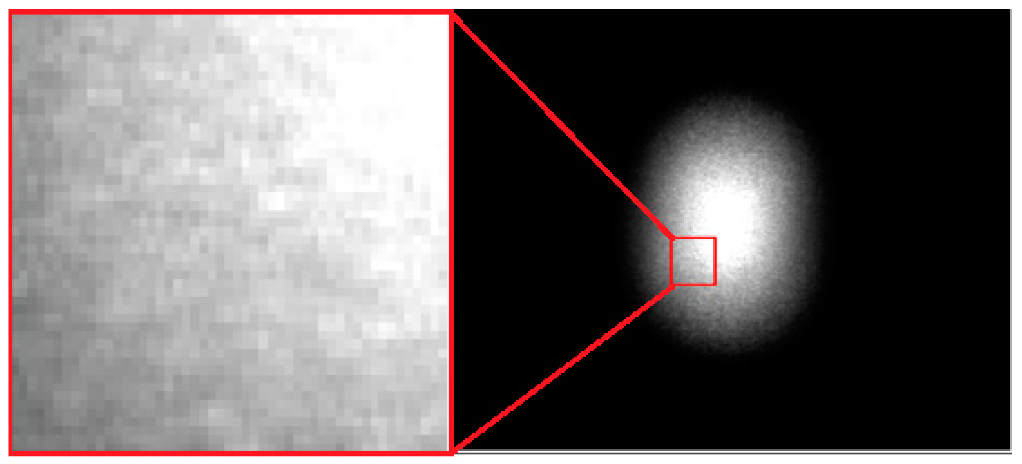
When the CCD camera obtains an image, as the light spot is located somewhere in the image, the range of the light spot image center will be searched preliminarily, as shown in Figure 2. After the region of the light spot is found by the program, the center point of the light spot region is displaced to overlap the CCD image center, and the magnification of the CCD is increased to coincide with the size of the light spot region. The light spot region is thus separated, and the first search is completed [16,17,18].

This system uses a convolutional neural network to search for the laser spot region. The neural network is trained using images with multiple complete light spots and incomplete light spot modes so that the program can judge the position of the light spot in the image accurately and rapidly.

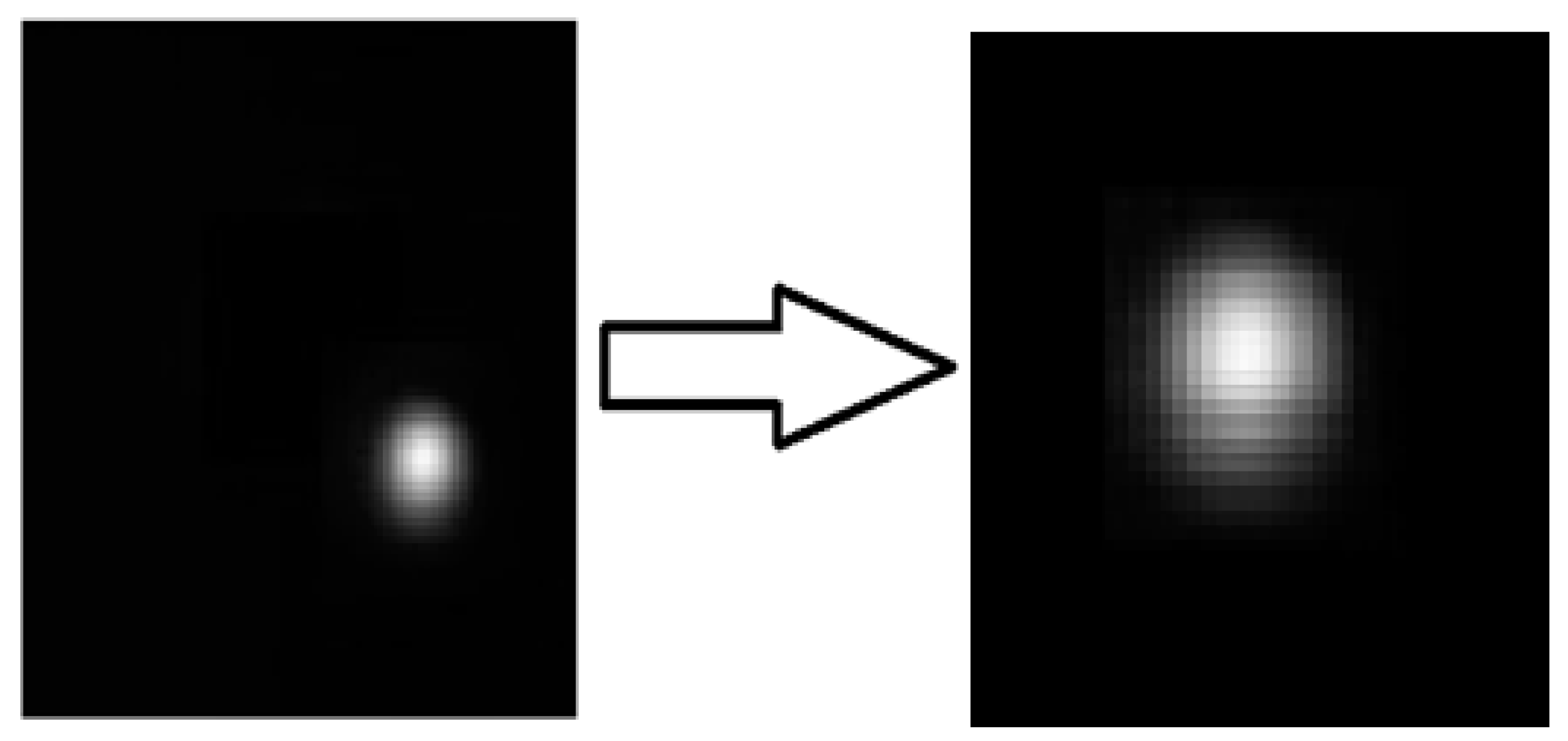
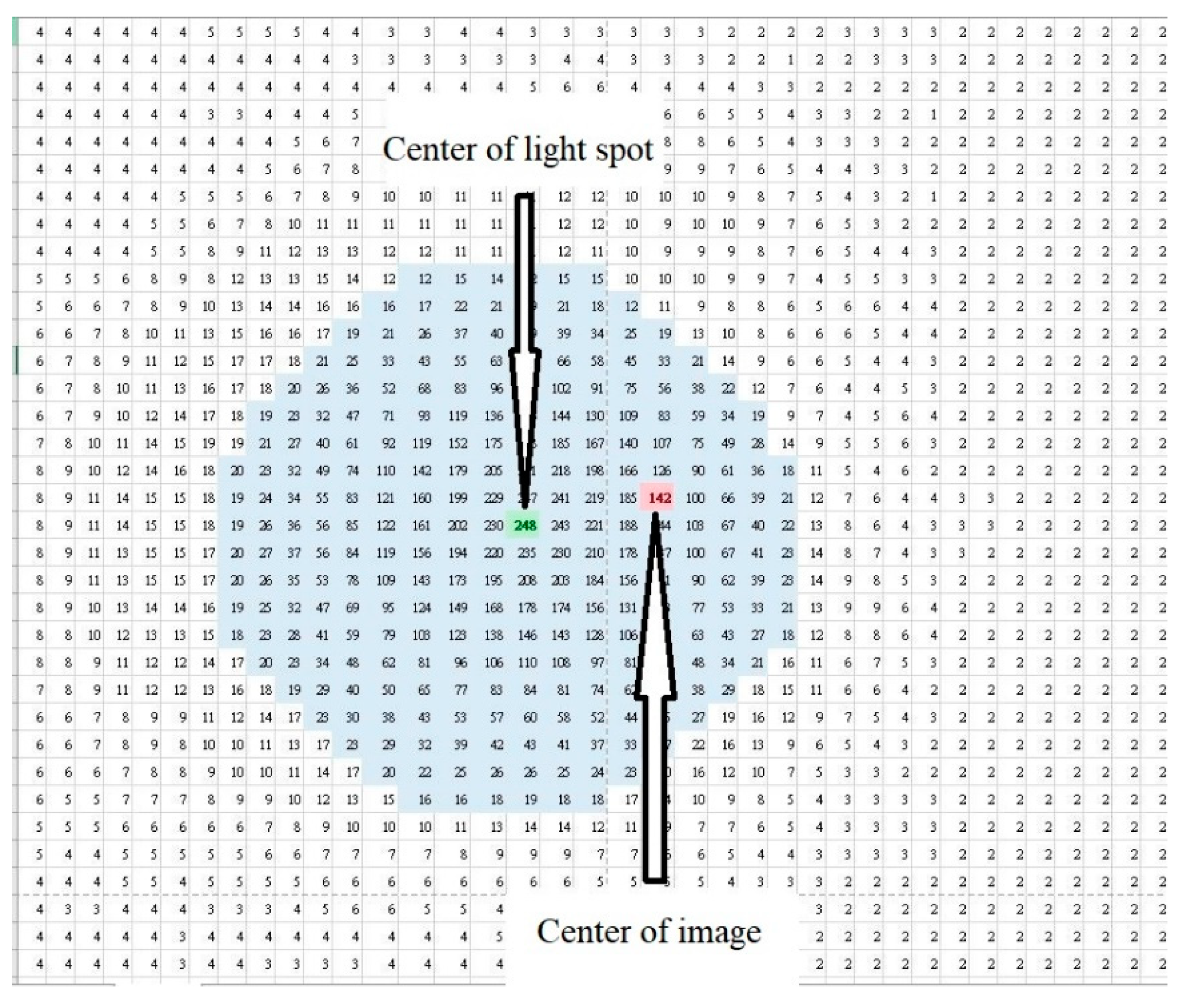
When the light spot region is positioned in the image successfully, the first part will use the center of the light spot region as the image center. This deviates from the actual light spot center, and the system will consider that the positioned laser spot region may not be a complete light spot, as shown in Figure 3. The distance between the CCD image center and the light spot center is measured, and the two centers are shifted and overlapped.

There are two processing modes, and whether the found light spot is complete or not is judged according to the aspect ratio of the light spot region. If it is a complete light spot, the centroid point of the light spot will be extracted using the centroid method, the distance between the CCD image center and the light spot center will be calculated, and the image center will be moved to overlap the light spot center. If it is not a complete light spot, the invariant moments will be calculated for the incomplete light spot region in the image and matched with the preset light spot source image to find out the position of the partial light spot region centroid in the light spot. The distance between the CCD image center and the light spot center is calculated, and the image center is moved to overlap the light spot center.

The positioning effects of this system with different sample numbers are described below. A total of 25, 50, and 100 positive samples were used to train the neural network.

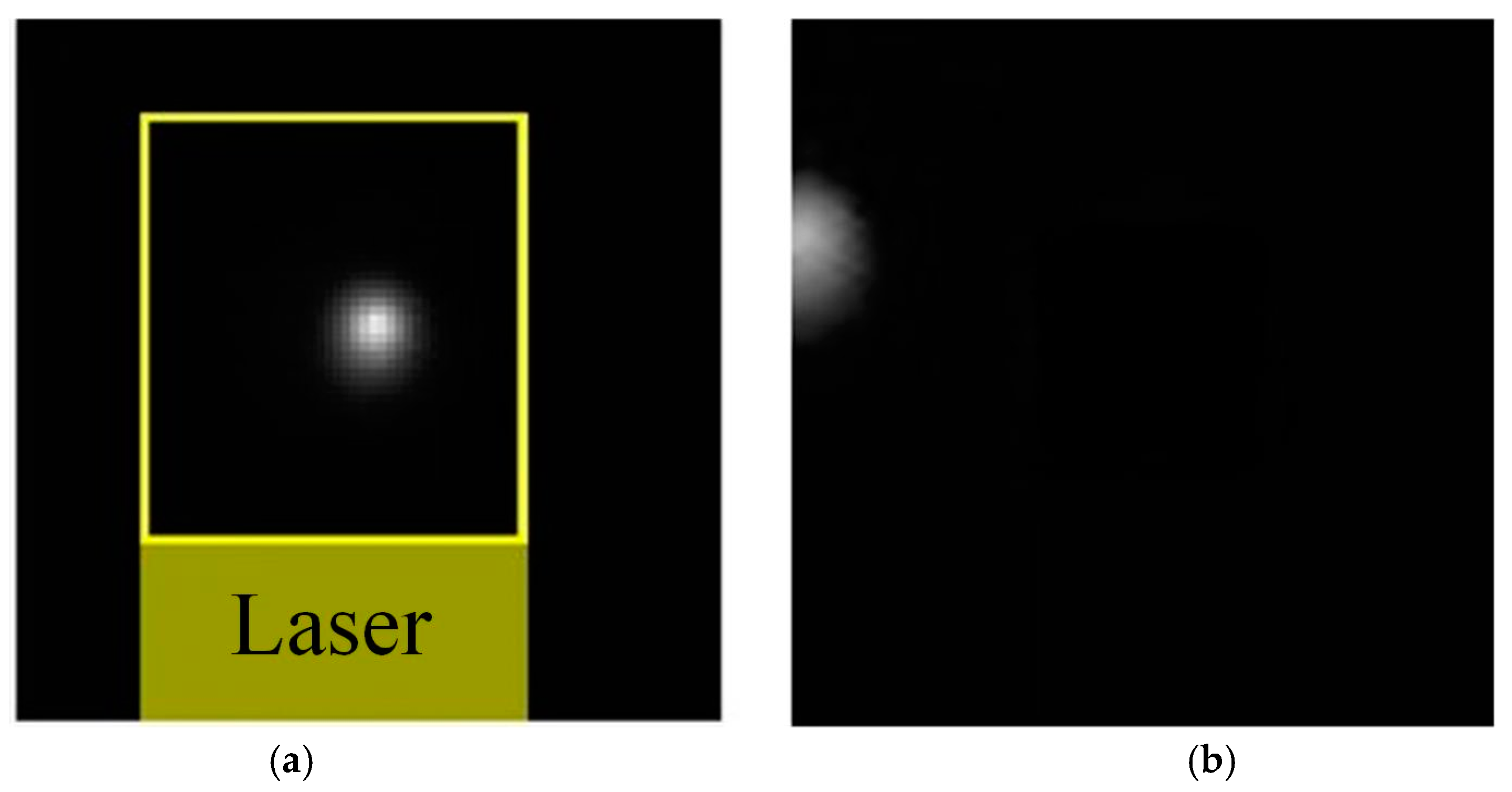
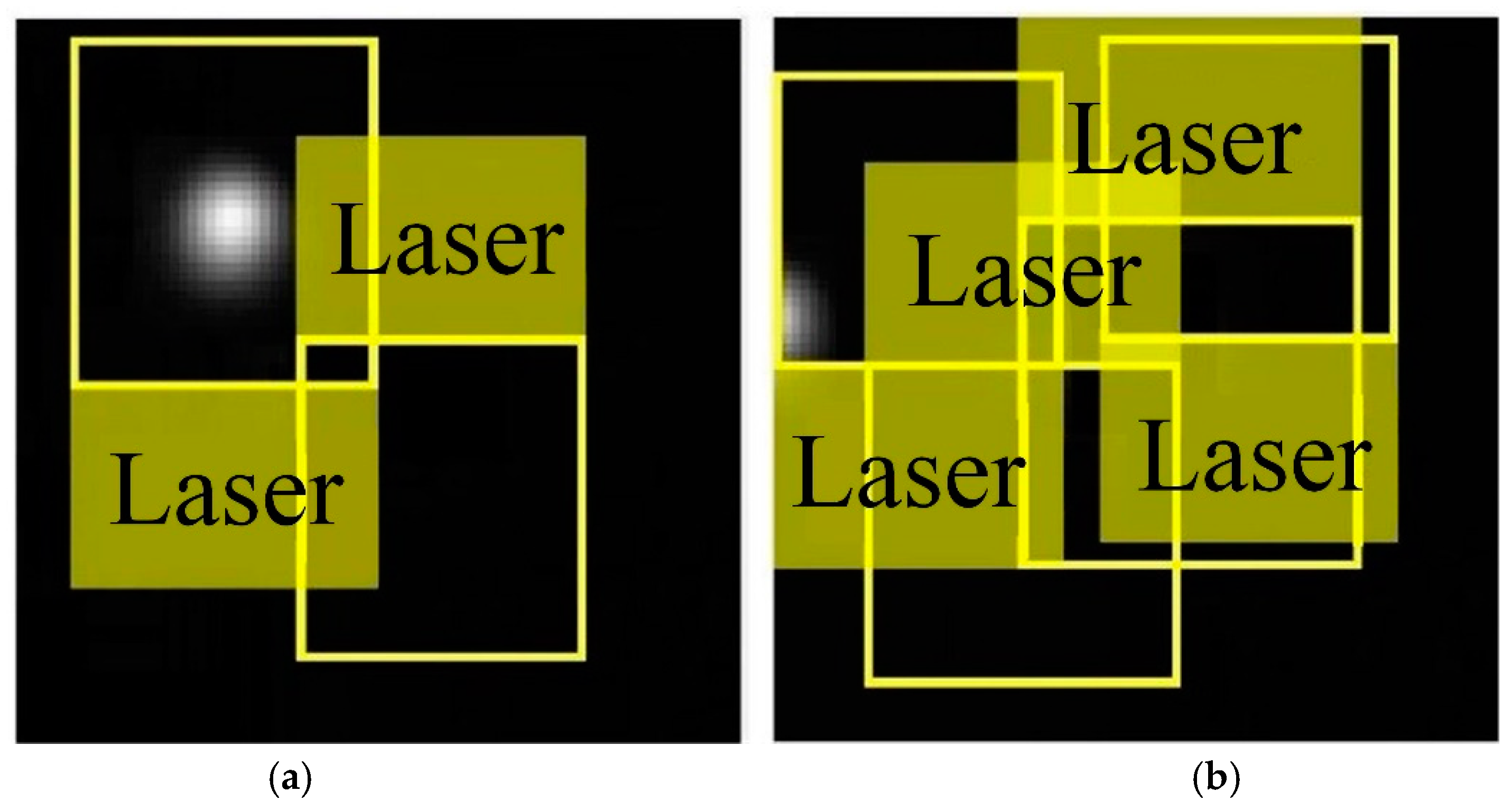
Figure 4 shows the program results of using 25 positive samples and 50 negative samples to train the neural network. According to Figure 4a, the program could position the complete light spot successfully, but there was still misrecognition. The incomplete light spot in Figure 4b could not be recognized successfully. In order to improve the results, this system increased the sample number and the program was trained again.

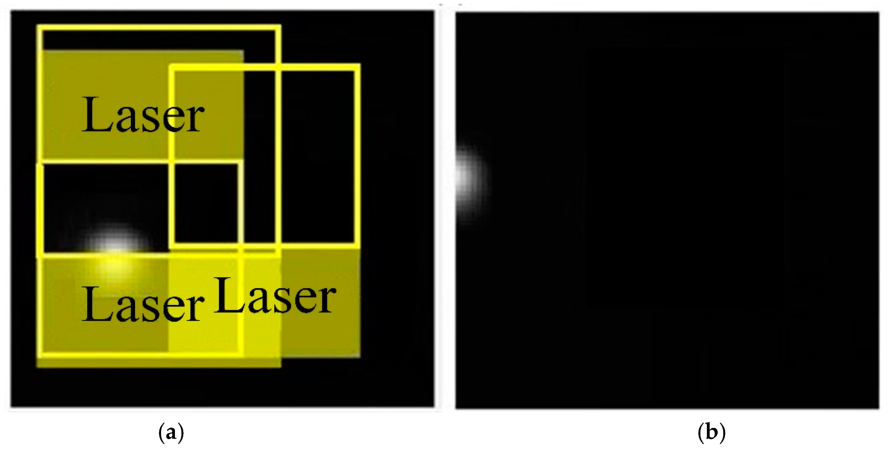
Figure 4 shows the program results of using 50 positive samples and 100 negative samples to train the neural network. Figure 5a shows that the misrecognition of complete light spots was improved, but it was unable to position the light spot region only. Figure 5b shows there were many misrecognitions but the position of incomplete light spots could be recognized. In order to further increase the accuracy, the sample number was increased a second time and the network was trained again.

After the neural network was trained using 100 positive samples and 200 negative samples, the program could position the region of complete light spots successfully. The misrecognition probability was reduced; however, it was still unable to position incomplete light spots.

Table 1. Experiment data of light spot positioning system.

Number of Positive Samples	25	50	100	100 (reduce feature region)
Number of Negative Samples	50	100	200	200
Number of Target Images	100	100	100	100
Result Candidates	74	90	96	98
Correct Results	40	69	88	96
Accuracy (%)	54.054	76.667	91.667	97.96
Classification Accuracy (μ)	0.37	0.284	0.245	0.14

shows the results of using three different sample numbers and changing the feature region size to train the neural network to recognize 100 target images. According to the data, the accuracy increased significantly with the sample number. The result candidates contained correct results and misrecognitions, and the result of the target images minus the result candidates showed that the program failed to recognize the number of targets.

According to Table 1, the system still had misrecognitions. This could be because the complete light spots and incomplete lights spots were recognized using the same neural network, or that the light spots were complete but only partial regions were positioned. In addition, when the laser was shot at the platform, the brightness would decrease outwards from the laser center spot, and the laser would be partially scattered by particles in the air. Visual recognition would be difficult because of the possibility of brightness in partial black regions. If the mode of these bright regions was close to the sample of the light spot, there could be misrecognition.

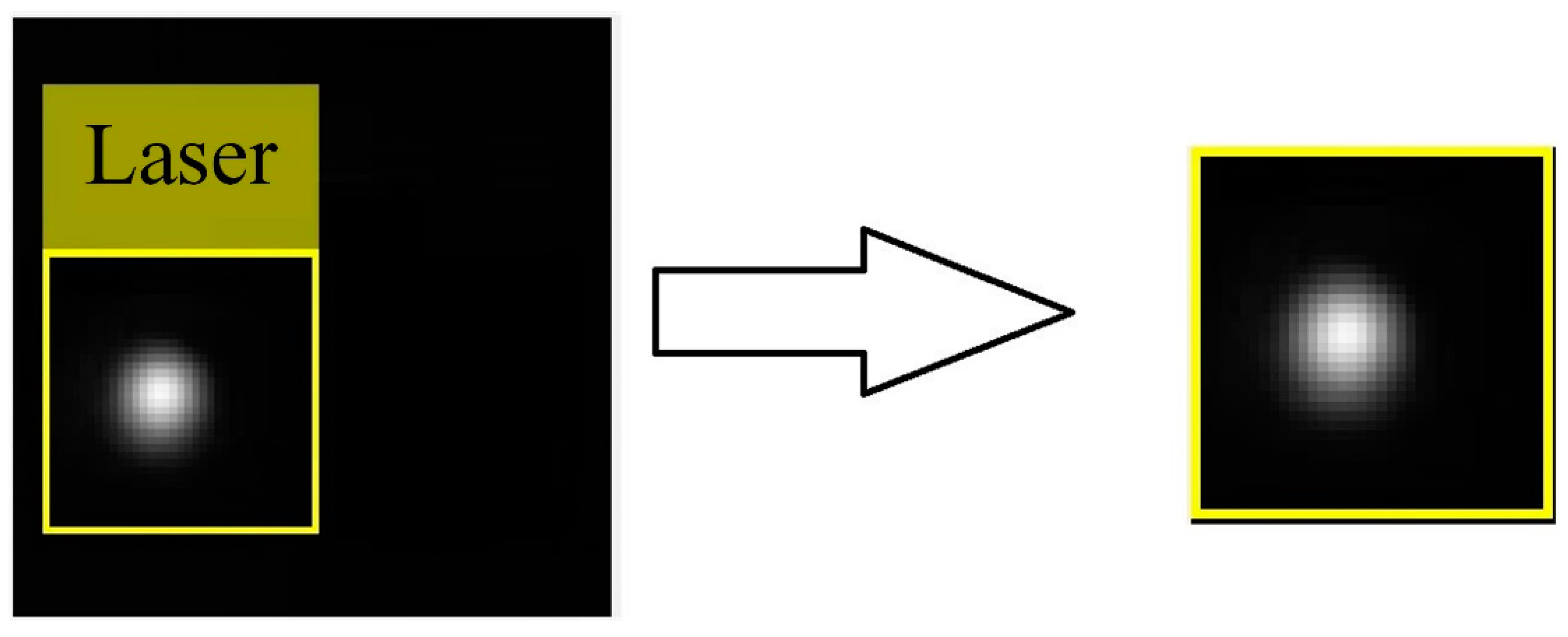
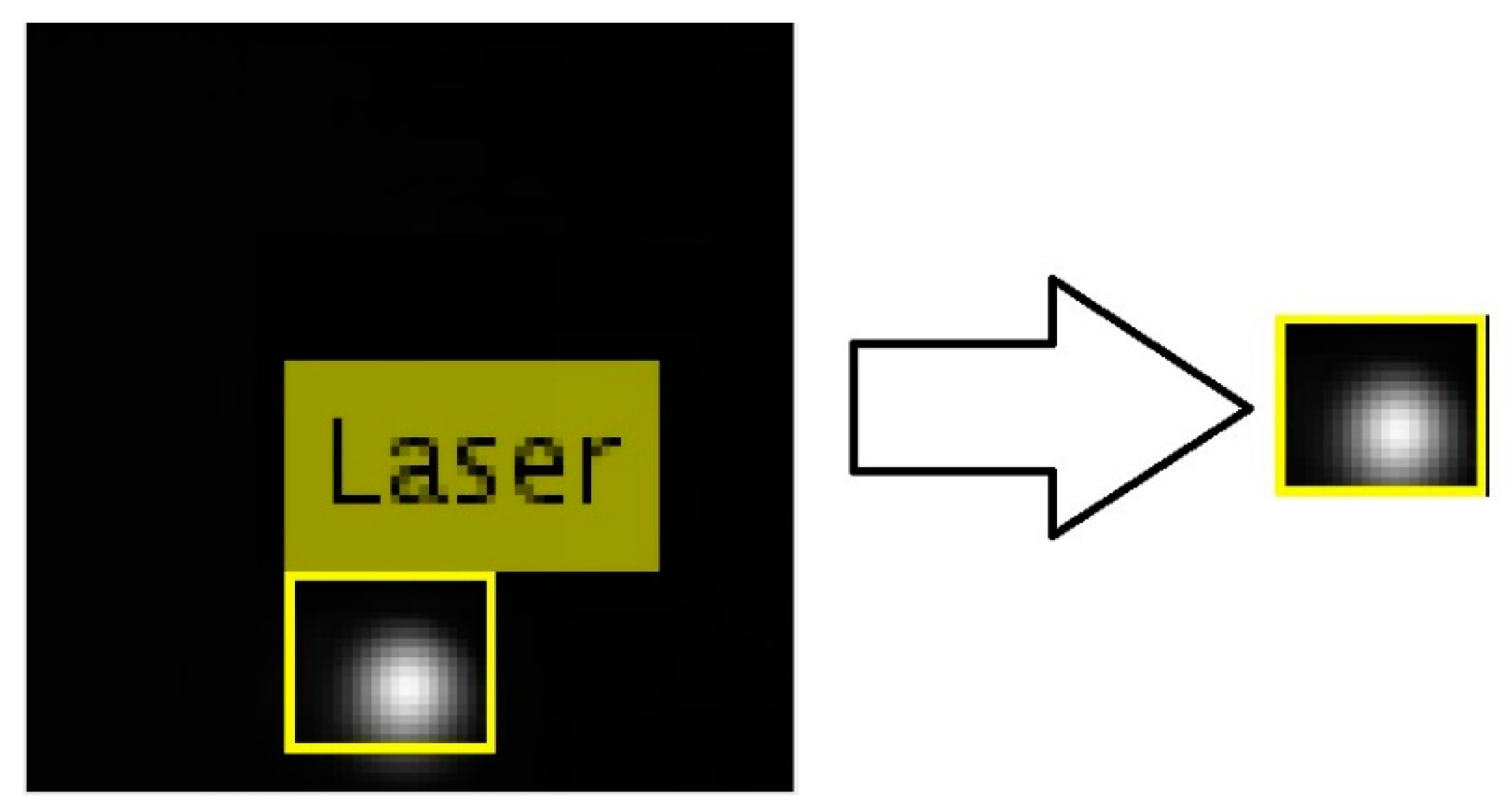
The region of the complete light spot was obtained successfully from the result of using 100 positive samples. According to the system flow, the CCD image center was moved to the positioning regional center and set as the template image, as shown in Figure 6.

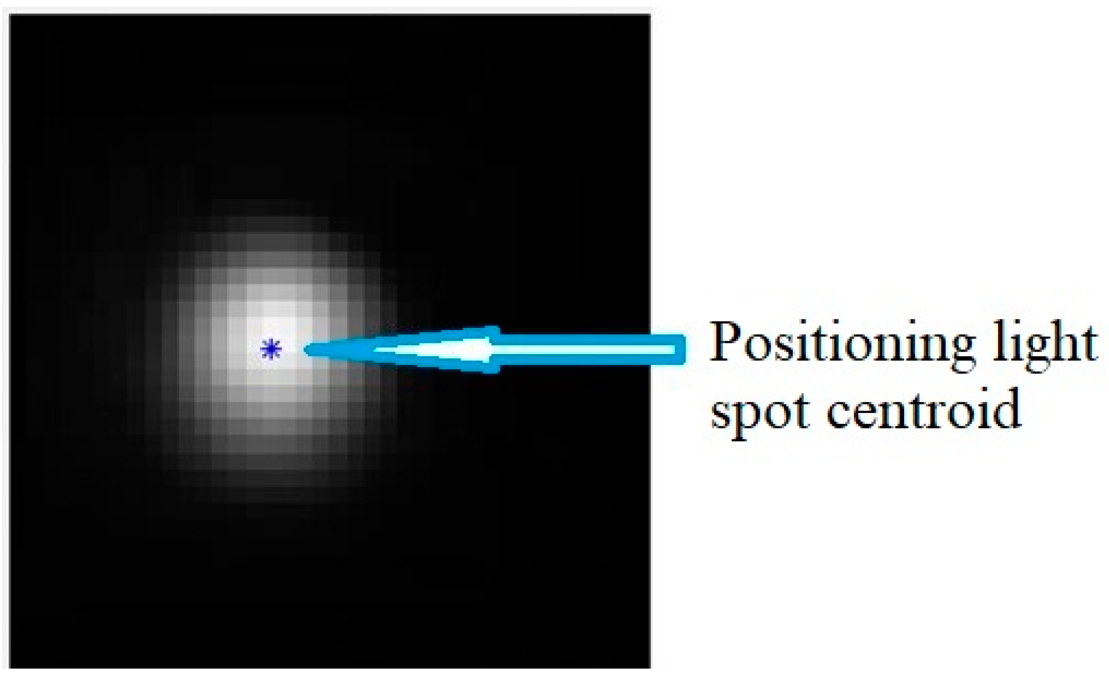
The aspect ratio of the region was calculated, and the aspect ratio of the template calculated by the program was 1.027. When the complete light spot was identified, the invariant moments of the template image were calculated and the first moment was taken, i.e., the barycentric coordinates of the light spot region, and these are indicated in the image, as shown in Figure 7.

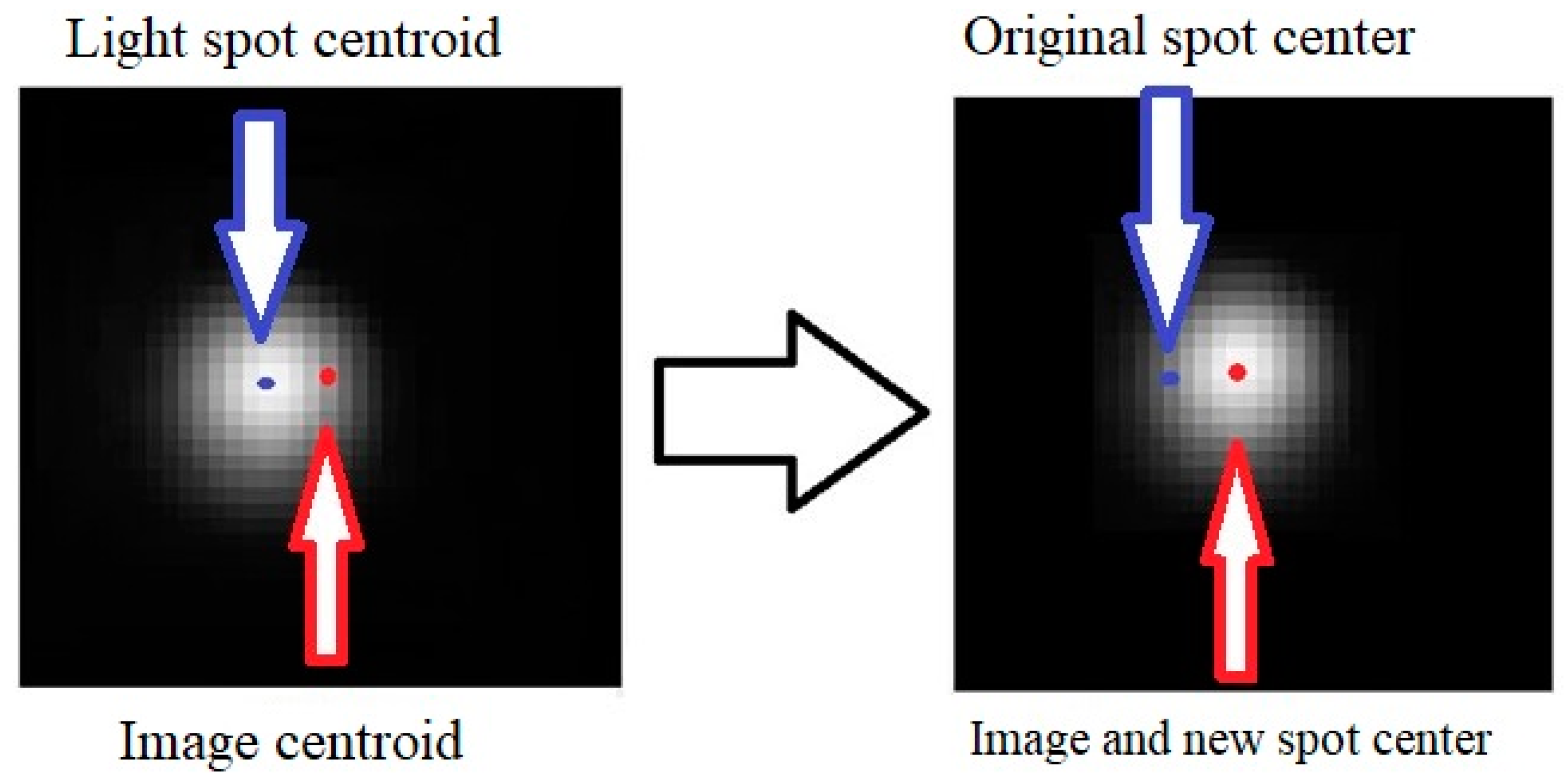
In the final step, the distance between the image center and the light spot center was calculated, and the CCD camera was moved. The image center and light spot center were overlapped, and the light spot center was aligned for the second time, as shown in Figure 8.

Figure 9 shows the gray level histogram of the laser spot. The positions of the light spot center and image center can be observed, and the distance between the two centers can be calculated by the coordinate relationship.

Table 2. Mean error of light spot positioning with different sample numbers.

Number of Positive Samples	25	50	100	100 (reduce region)
Average Mis-distance (pixel)	3.367	2.579	2.224	1.273
Average Mis-distance (µm)	0.37	0.284	0.245	0.14
Detection Time (s)	0.5 ~ 1.6	0.5 ~ 1.6	0.5 ~ 1.6	0.5 ~ 1.6

shows the mean errors of the image center and light spot center when the system performed light spot positioning with different sample numbers, where 1 pixel = 0.11 µm. It was observed that as the number of positive samples increased and the feature was enhanced, the center of the first positioning would be close to the center of the light spot and the time of the shift to the light spot center could be shortened.

Figure 10 is a recognized incomplete light spot map. First, it was recognized as being range independent, and the invariant moments were calculated using the image center as a reference point, as shown in

Table 3. Incomplete light spot invariant moments.

M1	M2	M3	M4	M5	M6	M7
0.3903	5.4796 × 10−4	5.1657 × 10−4	0.0077	−4.9596 × 10−6	1.3322 × 10−4	−1.4457 × 10−5

.

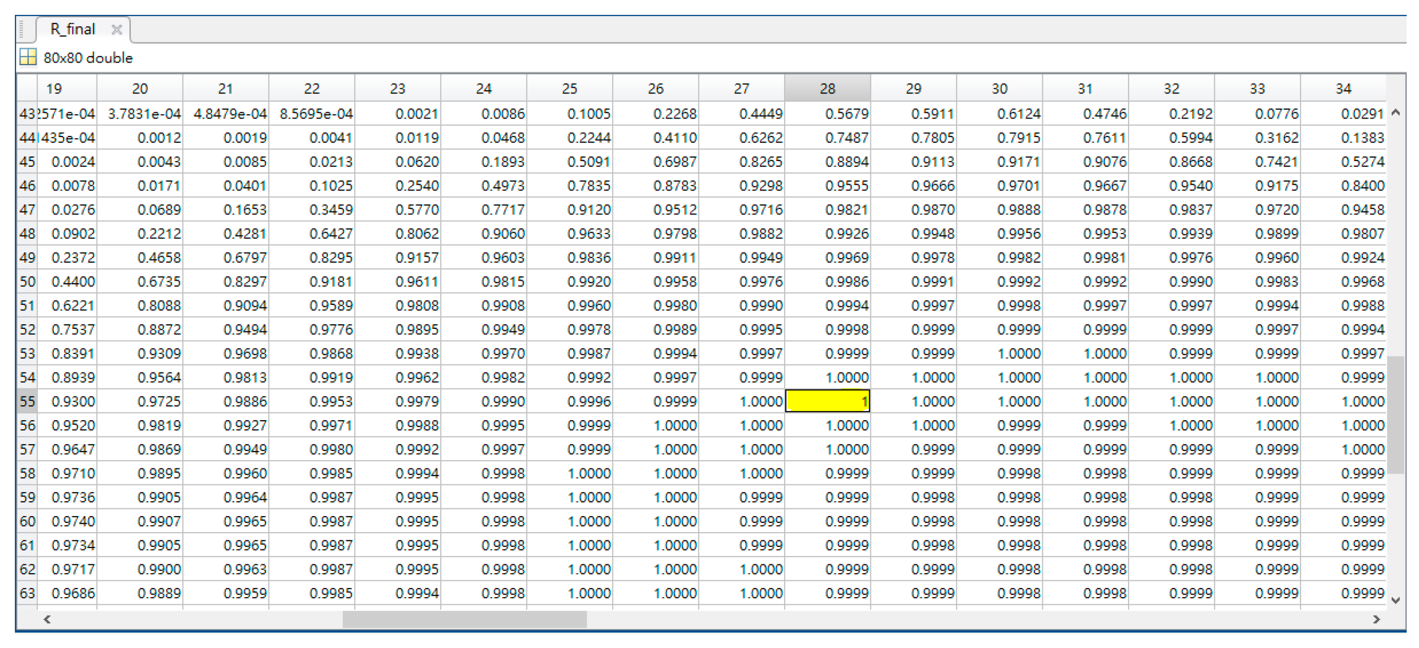
When the invariant moments of the recognition region were obtained, similarity matching was performed with the invariant moment matrix of all points in the complete light spot obtained in advance, and the coordinate value of the maximum matching weight was exported, as shown in Figure 11.

According to the above results, the position of the incomplete light spot image center in the complete light spot was obtained. Finally, as long as the distance between the image center and the complete light spot centroid was calculated and the position of the CCD was moved, the center point search could be completed (Figure 12).

5. Conclusions

In terms of the center spot search, compared with ordinary template matching, using invariant moments for matching was much faster. On the one hand, because the invariant moments digitized the image, the information to be processed at one time was 72% less than that for template matching using images for the operation. The invariant moment of every point of the source image would be calculated in advance and saved in a database as long as the invariant moments of the matched region were calculated, and the similarity to the database was calculated. Template matching generates a weighting matrix during matching and the weighting matrix must be created again whenever the template is changed, which takes considerable time.

The proposed system uses the aspect ratio to check whether the light spot is complete or not. The positioning method is selected according to the complete image of the light spot; thus, the complex computation of all images is unnecessary, and the load on the overall system is reduced.

References

- Bai, C.; Huang, L.; Pan, X.; Chen, S. Optimization of deep convolutional neural network for large scale image retrieval. Neurocomputing 2018, 303, 60–67. [Google Scholar] [CrossRef]
- Yu, X.; Fei, X. Target image matching algorithm based on pyramid model and higher moments. J. Comput. Sci. 2017, 21, 189–194. [Google Scholar] [CrossRef]
- Mehdi, K.; Massoud, P. Evaluation of morphological properties of railway ballast particles by image processing method. Transp. Geotech. 2017, 12, 15–25. [Google Scholar]
- Liu, X.; Lu, Z.; Wang, X.; Ba, D.; Zhu, C. Micrometer accuracy method for small-scale laser focal spot centroid measurement. Opt. Laser Technol. 2015, 66, 58–62. [Google Scholar] [CrossRef]
- Hanbay, K.; Talu, M.F.; Özgüven, Ö.F. Fabric defect detection systems and methods—A systematic literature review. Opt. Int. J. Light Electron Opt. 2016, 127, 11960–11973. [Google Scholar] [CrossRef]
- Chen, H. An efficient palmprint recognition method based on block dominat orientation code. Opt. Int. J. Light Electron Opt. 2015, 126, 2869–2875. [Google Scholar] [CrossRef]
- Zhang, Z.; Jaiswal, P.; Rai, R. FeatureNet: Machining feature recognition based on 3D Convolution Neural Network. Comput. Aided Des. 2018, 101, 12–22. [Google Scholar] [CrossRef]
- Hamuda, E.; Mc Ginley, B.; Glavin, M.; Jones, E. Automatic crop detection under field conditions using the HSV colour space and morphological operations. Comput. Electron. Agric. 2017, 133, 97–107. [Google Scholar] [CrossRef]
- Zhao, C.; Lee, W.S.; He, D. Immature green citrus detection based on colour feature and sum of absolute transformed difference (SATD) using colour images in the citrus grove. Comput. Electron. Agric. 2016, 124, 243–253. [Google Scholar] [CrossRef]
- Lee, J.-S.; Huang, B.-R.; Wei, K.-J. Preserving copyright in renovating large-scale image smudges based on advanced SSD and edge confidegnce. Opt. Int. J. Light Electron Opt. 2017, 140, 887–899. [Google Scholar] [CrossRef]
- Yoo, J.; Soo Hwang, S.; Dae Kim, S.; Seok Ki, M.; Cha, J. Scale-invariant template matching using histogram of dominant gradients. Pattern Recognit. 2014, 47, 3980. [Google Scholar] [CrossRef]
- Zhang, S.; Zhou, Y. Template matching using grey wolf optimizer with lateral inhibition. Opt. Int. J. Light Electron Opt. 2017, 130, 1229–1243. [Google Scholar] [CrossRef]
- Bao, G.; Cai, S.; Qi, L.; Xun, Y.; Zhang, L.; Yang, Q. Multi-template matching algorithm for cucumber recognition in natural environment. Comput. Electron. Agric. 2016, 127, 754–762. [Google Scholar] [CrossRef]
- Zhu, Y.; Qi, Q.; Mao, Y. A deep convolutional neural network approach to single-particle recognition in cryo-electron microscopy. BMC Bioinform. 2017, 18, 348. [Google Scholar] [CrossRef] [PubMed]
- Zhang, M.; Wu, J.; Lin, H.; Yuan, P.; Song, Y. The application of one-class classifier based on CNN in image defect detection. Procedia Comp. Sci. 2017, 114, 341–348. [Google Scholar] [CrossRef]
- Favorskaya, M.; Pyankov, D.; Popov, A. Motion estimations based on invariant moments for frames interpolation in stereovision. Procedia Comp. Sci. 2013, 22, 1102–1111. [Google Scholar] [CrossRef]
- Yang, J.; Wang, D.; Zhou, W. Precision laser tracking servo control system for moving target position measurement. Optik 2017, 131, 994–1002. [Google Scholar]
- Dhawan, R.; Dikshit, B.; Kawade, N. Development of a two-imensional fiber optic position sensor. Optik 2018, 169, 376–381. [Google Scholar] [CrossRef]
Figure 1.
Template matching result example.
Figure 2.
Schematic diagram of laser spot positioning.
Figure 3.
(a) Image of regional center that is not the light spot center; (b) incomplete laser spot image.
Figure 4.
(a) Complete light spot map positioning (25 positive samples); (b) incomplete light spot map positioning (25 positive samples).
Figure 5.
(a) Complete light spot map positioning (50 positive samples); (b) incomplete light spot map positioning (50 positive samples).
Figure 6.
Positioning region template.
Figure 7.
Positioning light spot centroid.
Figure 8.
Schematic diagram of the second alignment.
Figure 9.
Complete light spot gray level histogram.
Figure 10.
Incomplete light spot recognition map.
Figure 11.
Invariant moment similarity weighting matrix.
Figure 12.
Relative positions of incomplete light spot image center and light spot centroid.