Decision Support System for Medical Diagnosis Utilizing Imbalanced Clinical Data

Abstract

The clinical decision support system provides an automatic diagnosis of human diseases using machine learning techniques to analyze features of patients and classify patients according to different diseases. An analysis of real-world electronic health record (EHR) data has revealed that a patient could be diagnosed as having more than one disease simultaneously. Therefore, to suggest a list of possible diseases, the task of classifying patients is transferred into a multi-label learning task. For most multi-label learning techniques, the class imbalance that exists in EHR data may bring about performance degradation. Cross-Coupling Aggregation (COCOA) is a typical multi-label learning approach that is aimed at leveraging label correlation and exploring class imbalance. For each label, COCOA aggregates the predictive result of a binary-class imbalance classifier corresponding to this label as well as the predictive results of some multi-class imbalance classifiers corresponding to the pairs of this label and other labels. However, class imbalance may still affect a multi-class imbalance learner when the number of a coupling label is too small. To improve the performance of COCOA, a regularized ensemble approach integrated into a multi-class classification process of COCOA named as COCOA-RE is presented in this paper. To provide disease diagnosis, COCOA-RE learns from the available laboratory test reports and essential information of patients and produces a multi-label predictive model. Experiments were performed to validate the effectiveness of the proposed multi-label learning approach, and the proposed approach was implemented in a developed system prototype.

1. Introduction

With the huge improvement in human lifestyle and the increasingly aging population, there is a growing push to develop health services at a rapid speed [1]. In China, the number of patients visiting medical health institutions reached 7.7 billion in 2015, which was 2.3% higher than the previous year [2]. Worldwide, particularly in poor countries, the shortage of medical experts is severe, forcing clinicians to serve a large number of patients during their working time [3]. Generally, clinicians distinguish patients and diagnose their diseases using their experience and knowledge; however, in doing so, it is possible for clinicians without adequate experience to commit mistakes.

Information technology plays a vital role in changing human lifestyles. Rapid and drastic developments in the medical industry have been made utilizing information technology, and many medical systems have been produced to assist medical institutions to manage data and improve services. One survey report that medical informatics tools and machine learning techniques have been successfully applied to provide recommendations for diagnosis and treatment. Therefore, automatic diagnosis is a key focus in the domain of medical informatics.

It is common for a patient to suffer from more than one disease due to medical comorbidities. For instance, diabetes mellitus type 2 and hyperlipoidemia are likely to give rise to cardiovascular diseases [4,5]. In fact, it has been found that a majority of patients are diagnosed as suffering from more than one disease. Automatic diagnosis suggests some possible illnesses rather than just a single illness, and the disease diagnosis problem is accordingly transferred into a multi-label learning problem. Wang et al. [6] proposed a shared decision-making system for diabetes medication choice using a multi-label learning method to recommend multiple medications among eight classes of available antihyperglycemic medications. However, in this system, each label is considered independently, and label correlations are not considered. Cross-Coupling Aggregation (COCOA) [7] is a typical multi-label learning approach aimed at leveraging label correlation and exploring class imbalance. For each label, COCOA aggregates the predictive result of a binary-class learner for this label and predictive results of some multi-class learners for the pairs of this label and other labels. However, class imbalance may still affect a multi-class imbalance learner when the number of a coupling label is too small.

To improve the performance of COCOA, a regularized ensemble approach integrated into multi-class classification process of COCOA named as COCOA-RE is presented in this paper. Considering the problem of class imbalance, this method leverages a regularized ensemble method [8] to explore disease correlations and integrates the correlations among diseases in the multi-label learning process. To provide illness diagnosis, COCOA-RE learns from the available laboratory test reports and essential information of patients and produces a multi-label predictive model. As part of this study, experiments were performed to validate the effectiveness of the proposed multi-label learning approach, and the proposed approach was implemented in a developed system prototype. The proposed system—shown in Figure 1—can help clinicians review patient conditions more comprehensively and can provide more accurate suggestions of possible diseases to clinicians.

Figure 1. Overview of the decision support system for medical diagnosis.

The rest of this paper is organized as follows: Section 2 presents the existing work about multi-label learning approaches for class-imbalanced data sets. Section 3 describes the proposed multi-label learning approach. Section 4 discusses the experimental results. Finally, Section 5 concludes our work with a summary.

2. Related Work

Clinical decision support systems—of which diagnosis decision support system is a representative example—are developed to assist clinicians in making accurate clinical decision using informatics tools and machine leaning techniques [9]. Boosting approaches [10], support vector machines (SVMs) [11], deep learning [12] and rule-based methods [13] have been applied in clinical decision support systems for detecting specific diseases. However, multi-label learning approaches are rarely applied in clinical decision support systems. One example where this type of learning approach was used was in Wang et al. [6]. Using electronic health record data and applying the multi-label learning approach, the authors of that paper developed a shared decision-making system for recommending diabetes medication.

According to the order of label correlation considered by the multi-label learning methods, existing approaches are divided into three categories—first-order strategy, second-order strategy, and high-order strategy. First-order strategy considers each label independently and does not take into account correlations among labels. Binary relevance (BR) [14]—a popular approach in most advanced multi-label learning algorithms—constructs an independent binary classifier for each label to achieve multi-label learning. It is easy to apply BR, but the performance of BR cannot be improved by considering correlations among labels. Multi-label learning K-nearest neighbor (ML-KNN) [15], which maximizes posterior probability to predict the labels of target examples, is a simple and effective approach for multi-label learning. Multi-Label Decision Tree (ML-DT) [16] adapts decision tree methods and produces the tree using information gained according to multi-label entropy in multi-label learning. Second-order strategy, e.g., Collective Multi-Label Classifier (CML) [17], Ranking Support Vector Machine (Rank-SVM) [18], and Calibrated Label Ranking(CLR) [19], considers correlations between a pair of labels in the learning process. For multi-label data with m labels, CLR makes m(m−1) binary classifiers, one of which is for a pair of labels. Rank-SVM produces a group of linear classifiers in the multi-label scenarios using the maximum margin principle to minimize the empirical ranking loss. To train multi-label data, CML applies maximum entropy principle to make the resulting distribution satisfy a constrain of correlations among labels. High-order strategy considers correlations among all class labels or subsets of class labels. RAndom k-labELsets (RAKEL) [20] transfers the multi-label learning task into an ensemble multi-class learning task in which each multi-class learner only handles a subset of randomly selected k labels.

Some examples are normally associated with more than one label in many multi-label learning tasks. However, the number of negative examples is much larger than that of positive examples in some labels, which brings about the problem of class imbalance in multi-label learning.

Class imbalance is a well-known threat in traditional classification methods [21,22,23]; however, it has not been extensively studied in the multi-label learning context. The existing methods towards class imbalance can be grouped into two categories. In the first case, multi-label learning methods transfer the class-imbalanced distribution into class-balanced distribution using data resampling, creating (over-sampling), or removing (under-sampling) data examples. For example, a multi-label synthetic minority over-sampling technique (MLSMOTE) [24] has been developed to produce synthetic examples associated to minority labels for imbalanced multi-label data. In this approach, the features of new examples are generated by interpolations of values belonging to the nearest neighbors. In the second case, a cost-sensitive multi-label learning is made up of two different classification approaches, such as binary-class imbalance classifier and multi-class imbalance classifier. To handle the problem about class imbalance and concept drift in multi-label stream classification, Xioufis et al. [25] used a multiple window method. By combing labels, Fang et al. [26] proposed a multi-label learning method called DEML (Dealing with labels imbalance by Entropy for Multi-Label classification). To leverage the exploration of class imbalance and the exploitation of label correlation, a multi-label learning approach called Cross-Coupling Aggregation (COCOA) [7] has also been proposed. Although the effectiveness of COCOA has been validated, the class imbalance may still affect a multi-class imbalance learner when the number of a coupling label is too small.

To handle class-imbalanced training data, many multi-class approaches have been developed. In general, the existing approaches can be categorized as data-adaption approaches and algorithmic-adaption approaches [27,28,29]. In data-adaption approaches, the minority class examples and majority class examples are balanced by sampling strategies, e.g., under-sampling or over-sampling. The over-sampling process creates synthetic examples corresponding to minority examples, whereas the under-sampling process reduces the number of majority examples. To create synthetic examples, some techniques apply random pattern, while others follow density distribution [30]. Algorithmic-adaption approaches involve approaches that adapt to imbalanced data. For example, cost-sensitive learning approaches spend higher cost in learning minority class [31]. Boosting methods integrate sampling and algorithmic-adaption approaches to deal with class-imbalanced data sets. AdaBoost [32] was developed to sequentially learn multiple classifiers and integrate them to achieve better performance by minimizing an error function. AdaBoost can not only be used to one-class classification but also multi-class classification. AdaBoost is able to be directly applied to multiple binary classifications transformed by multi-class classification, e.g., AdaBoost.M2 [32] and AdaBoost.MH [33]. In these approaches, higher costs and extended training time are required to learn many weak classifiers, and the accuracy will be limited if the number of classes are large. AdaBoost.M1 directly generalizes AdaBoost into multi-class classification, but it requires the accuracy of each weak classifier larger than a strict error bound. Stage-wise Additive Modeling using Multi-class using Multi-class exponential (SAMME) loss function [34] has been used to extend AdaBoost methods to multi-class classification. SAMME eases the accuracy of each weak classifier in AdaBoost.M1 from 1/2 to 1/k so that the weak classifier whose performance is better than random guesses is accepted. However, these multi-class boosting approaches neglect the deterioration of classification accuracy in the training process. A regularized ensemble framework [8] was therefore introduced to learn multi-class imbalanced data sets. To adapt multi-class imbalanced data sets, a regularization term is applied to automatically adjust every classifier’s error bound according to its performance. Furthermore, the regularization term will penalize the classifier if it incorrectly classifies examples that had been classified correctly by the previous classifier.

3. Proposed Methodology

In multi-label learning, each example is described by a feature vector while being associated with multiple-class labels simultaneously. $\mathrm{X}={ℝ}^d$ is the dimension of features and $\mathrm{Y}={ℝ}^q$ is the dimension of labels. Given a multi-label data $D=\{(X_i,Y_i)|1\le i\le N\}$, where $X_i=(x_1,x_2,\dots x_d)$ denotes a d-dimensional feature vector of the example, $i$ and $x_i^j$ are the values of $X_i$ in feature $f_j$, and $Y_i=(y_1,y_2,\dots y_q)$ denotes the label vector of the example $i$. $y_i^j=1$ when $X_i$ has label $l_j$; otherwise, $y_i^j=0$. The task of multi-label learning is to learn a multi-label classifier $h:\mathrm{X}\to 2^{\mathrm{Y}}$ from $D$, which maps the space of feature vectors to the space of label vectors. In addition, most of the existing multi-label learning methods do not fully consider the class imbalance among labels. For class label, the positive training examples are denoted by $D_j^{+}=\{(x_i,1)|y_i\in Y_i,1\le i\le N\}$ and the negative training examples are denoted by $D_j^{-}=\{(x_i,0)|y_i\in Y_i,1\le i\le N\}$. As a general rule, it is possible for the imbalance ratio $\mathrm{Im}R=\max (|D_j^{+}|,|D_j^{-}|)/\min (|D_j^{+}|,|D_j^{-}|)$ to become high because $|D_j^{+}|$ is less than $|D_j^{-}|$ in most cases. Therefore, the corresponding imbalance ratio is used to measure the imbalance of multi-label data. Considering multi-label imbalanced data sets, COCOA is an effective multi-label learning approach to train an imbalanced clinical data set in the proposed technique. In this study, a regularized ensemble approach integrated into multi-class classification process of COCOA named as COCOA-RE was developed to improve the performance of COCOA.

3.1. Data Standardization

Prior to the multi-label learning process, it is necessary to standardize the value of whole features. Owing to the fact that all features may be presented by different data types and their values may belong to different ranges, the features with higher range values participate more heavily in the training process than the features with lower range values as it would contribute to bias. Therefore, it is necessary to perform data standardization. Min–Max scaling of all values in the range of [0, 1] is performed as:

$$x_i^{\ast }=\frac{x_i-x_{\max }}{x_{\max }-x_{\min }}$$

(1)

where $x^{\ast }$ is the standardized feature, $x_{\max }$ is the maximum value of corresponding feature before the standardization, and $x_{\min }$ is the minimum value of corresponding feature before the standardization.

3.2. COCOA Method for Class-Imbalanced Data

The task of multi-label learning is to learn a multi-label classifier $h:\mathrm{X}\to 2^{\mathrm{Y}}$ from the training set. In other words, this is for learning $q$ real-valued functions $f_j:\mathrm{X}\to ℝ(1\le j\le q)$, and each function is combined with a threshold $t_j:\mathrm{X}\to ℝ$. For each inputting example $x\in \mathrm{X}$, $f_j(x)$ denotes a confidence of relating $x$ to class label $y_j$, and the predictive class label set is established as follows:

$$h(x)=\{y^j|f_j(x)>t_j(x),1\le j\le q\}$$

(2)

For the class label $y_j$, $D_j$ denotes the binary training set from original training set $D$:

$$\begin{array}{l}{D}_j=\{(x_i,\varphi (Y_i,y_j))|1\le i\le N\}\\ \mathrm{where}\varphi (Y_i,y_j)=\{\begin{array}{c}+1,\mathrm{if}{y}_j\in Y_i\\ -1,\mathrm{otherwise}\end{array}\end{array}$$

(3)

Instead of learning a binary classifier from $D_j$, i.e., $g_j\leftarrow B(D_j)$, which considers that labels are independent, COCOA tries to incorporate label correlations in the learning classification model. In COCOA, another class label $y_k(k\ne j)$ is randomly selected to couple with $y_j$. Given the label pair $(y_j,y_k)$, a multi-class training set is presented as follows:

$$\begin{array}{l}{D}_{jk}=\{(x_i,\phi (Y_i,y_j,y_k))|1\le i\le N\}\\ \mathrm{where}\phi (Y_i,y_j,y_k)=\{\begin{array}{c}0,\mathrm{if}{y}_j\notin Y_i\mathrm{and}{y}_k\notin Y_i\\ +1,\mathrm{if}{y}_j\notin Y_i\mathrm{and}{y}_k\in Y_i\\ +2,\mathrm{if}{y}_j\in Y_i\mathrm{and}{y}_k\notin Y_i\\ +3,\mathrm{if}{y}_j\in Y_i\mathrm{and}{y}_k\in Y_i\end{array}\end{array}$$

(4)

Supposing that the minority class in binary training set $D_j$/$D_k$ corresponds to the positive examples of label $y_j$/$y_k$, the first class and the fourth class in $D_{jk}$ would consist of largest and smallest number of examples. While the original imbalance ratios in binary training sets are $\mathrm{Im}{R}_j$ and $\mathrm{Im}{R}_k$, respectively, the imbalance ratio would roughly turn into $\mathrm{Im}{R}_j\cdot \mathrm{Im}{R}_k$ in four-class training set $D_{jk}$, which implies that the worst-case imbalance ratio in a four-class training set would be much larger than that in a binary training set. To deal with this problem, COCOA converts the four-class training set into tri-class training set as follows:

$$\begin{array}{l}{D}_{jk}^{tri}=\{(x_i,{\phi }^{tri}(Y_i,y_j,y_k))|1\le i\le N\}\\ \mathrm{where}{\phi }^{tri}(Y_i,y_j,y_k)=\{\begin{array}{l}0,\mathrm{if}{y}_j\notin Y_i\mathrm{and}{y}_k\notin Y_i\\ +1,\mathrm{if}{y}_j\notin Y_i\mathrm{and}{y}_k\in Y_i\\ +2,\mathrm{if}{y}_j\in Y_i\end{array}\end{array}$$

(5)

In this case, for the new third class, its imbalance ratio of the first class and that of the second class would roughly turn into $\frac{\mathrm{Im}{R}_j\cdot \mathrm{Im}{R}_k}{1+\mathrm{Im}{R}_k}$ and $\frac{\mathrm{Im}{R}_j}{1+\mathrm{Im}{R}_k}$, which are much smaller than the imbalance ratio $\mathrm{Im}{R}_j\cdot \mathrm{Im}{R}_k$ of the worst case in a four-class training set.

By applying a multi-class learner on $D_{jk}^{tri}$, the multi-class classifier can be induced as $g_{jk}\leftarrow M(D_{jk}^{tri})$. $g_{ik}(+2|x)$ represents the predictive confidence that example $x$ ought to have positive assignment of label $i$, regardless of $x$ having positive or negative assignment of label $k$. In COCOA, a subset of $K$ class labels $L_k\subseteq Y\backslash y_j$ is selected randomly for each class label for pairwise coupling. The predictive confidences of a binary-class learner and $K$ multi-class learners aggregate to determine the real-value function $f_j(x)$:

$$f_j(x)=g_j(+1|x)+{\displaystyle {\sum }_{y_k\in L_k}{g}_{ik}(+2|x)}$$

(6)

COCOA chooses a constant function $t_j(x)=a_j$ to set the thresholding function $t_j(\cdot )$. Any example $x$ is predicted to have positive assignment of label $j$ if $f_j(x)>a_j$ and vice versa. F-measure metric is employed to find out the appropriate thresholding constant $a_j$ as follows:

$$a_j=\arg {\max }_{a\in ℝ}F(f_j,a,D_j)$$

(7)

where $F(f_j,a,D_j)$ denotes the value of F-measure calculated by employing $\text{{}{f}_j,a\text{}}$ on $D_j$.

3.3. Regularized Boosting Approach for Multi-Class Classification

In each iteration of ensemble multi-class classification model, some examples are classified incorrectly by the current classifier after being classified correctly by the classifier in the previous iteration; in particular, the distribution of multiple classes is imbalanced. A regularization parameter was introduced by Yuan et al. [32] into the convex loss function to calculate the classifier weight. This parameter penalized the weight of the current classifier if the classifier misclassifies examples that were classified correctly by the previous classifier. The regularized multi-class classification method aims to keep the correct classifications of minority examples, control the decision boundary towards minority examples, and prevent the bias derived from the large amount of majority examples.

After each learning iteration, the weight of current classifier is calculated as follows:

$${\alpha }_t=\frac{1}{2}\log (\frac{1-e_t}{e_t})+\frac{1}{2}\log ({\delta }_t(C-1))$$

(8)

where the regularization parameter ${\delta }_t$ is initialized as 1. According to the loss function, the weights of misclassified examples are adjusted to increase while the weights of those classified correctly are adjusted to decrease. The weights of examples are updated as follows:

$$w_t=\{\begin{array}{c}{w}_{t-1}(i)e^{-{\alpha }_t},\forall x_i,f_i(x_i)=y_i\\ w_{t-1}(i)e^{{\alpha }_t},\forall x_i,f_i(x_i)\ne y_i\end{array}$$

(9)

After updating the weights of examples, the weights would be normalized.

Misclassified examples are categorized into two classes: (i) second-round-misclassified examples $X_c=\{x_i;f_t(x_i)\ne y_i\mathrm{and}{f}_{t-1}(x_i)=y_i\}$, which are classified incorrectly by current classifier but classified correctly by previous classifier; and (ii) two-rounds-misclassified examples $X_m=\{x_i;f_t(x_i)\ne y_i\mathrm{and}{f}_{t-1}(x_i)\ne y_i\}$, which are classified incorrectly by both the current classifier and the previous classifier. The weighted error is calculated by misclassified examples as follows:

$$\begin{array}{l}{e}_t={\displaystyle \sum _{i\in X_c}{w}_{t-1}(i)}+{\displaystyle \sum _{i\in X_m}{w}_{t-1}(i)}\\ ={{\displaystyle \sum _{i\in X_c}{w}_{t-2}(i)(\frac{{\delta }_{t-1}(C-1)(1-e_{t-1})}{e_{t-1}})}}^{-\frac{1}{2}}+{{\displaystyle \sum _{i\in X_m}{w}_{t-2}(i)(\frac{{\delta }_{t-1}(C-1)(1-e_{t-1})}{e_{t-1}})}}^{\frac{1}{2}}\end{array}$$

(10)

The regularization term penalizes the current classifier that had misclassified the second-round-misclassified examples by changing its weight. To derive the regularization term, it assumes that all examples misclassified by the current classifier are also misclassified by the previous classifier. Thus, the exponent in expression of calculating the error of second-round-misclassified examples transfers into positive. In the above assumption, the maximum possible error is computed as follows:

$$e_t^{\ast }={\displaystyle \sum _{i\in (X_c\cup X_m)}{w}_{t-2}(i)(\frac{{\delta }_{t-1}(C-1)(1-e_{t-1})}{e_{t-1}}}{)}^{\frac{1}{2}}$$

(11)

Then, the expression of the actual weighted error is computed as follows:

$$e_t=e_t^{\ast }{\delta }_t^{\frac{1}{2}}$$

(12)

Accordingly, the explicit expression of regularization term can be derived as follows:

$${\delta }_t=\frac{e_t^2{e}_{t-1}}{({\displaystyle \sum _{i\in X_c\cup X_m}{w}_{t-2}(i){)}^2(1-e_{t-1}){\delta }_{t-1}(C-1)}}$$

(13)

Both weighted error and regularization term are used to compute the weight of current classifier as shown in Equation (5). The regularization term is adjusted in each iteration in terms of the performances of the current classifier and the previous classifier. Considering this scheme, the weighted error needs to follow the below equation:

$$(1-e_t)\delta (C-1)>e_t$$

(14)

Thus, the weighted error boundary of the current classifier t is as follows:

$$e_t<\frac{1}{1+{\delta }_t^{-1}{(C-1)}^{-1}}$$

(15)

3.4. COCOA Integrated with a Regularized Boosting Approach for Multi-Class Classification

Class imbalance still exists in $D_{jk}^{tri}$ when the number of examples with label $j$ or the number of examples with label $k$ is too small. Therefore, it is necessary to apply a multi-class classifier that is able to handle multi-class imbalanced data sets in $D_{jk}^{tri}$. In this study, a regularized boosting approach introduced in Section 3.3 was integrated into the process of multi-class classification in COCOA (named as COCOA-RE) to achieve better performance.

Table 1 presents the COCOA-RE method. For each label, a binary-class classifier and $\mathrm{K}$ coupling multi-class classifiers were performed to train the multi-label data set. Instead of using a single multi-class classifier, a regularized boosting approach was applied to produce an ensemble classifier for the training data set of each coupling labels. The regularization parameter was initialized to be equal at 1, and the weight of each example was initialized with $1/M$. Two indicator functions were used in the COCOA-RE approach, namely Function $1_0^1$ and Function $1_{-1}^1$. Function $1_0^1$ was equal at 1 if true, 0 otherwise, and it was used in calculation of the weighted error. Function $1_{-1}^1$ was equal at 1 if true, −1 otherwise, and it was used to update the weight of examples. After training the multi-label data set, the predictive value for label $y_j$ was integrated by the predictive confidences calculated by the binary-class classifier and multi-class classifiers. Eventually, the predictive models of all labels were performed to produce the predicted label set for the testing example.

Table 1. The pseudo-code of (COCOA-RE). COCOA-RE: a regularized ensemble approach integrated into multi-class classification process of COCOA; COCOA: Cross-Coupling Aggregation.

Algorithm: COCOA-RE

Inputs:  $D$: the multi-label training set $T=\{(X_1,Y_1),(X_2,Y_2),\dots ,(X_n,Y_n)\}$  $B$: the binary-class classifier  $M$: the multi-class classifier  $K$: the number of coupling labels  $x$: the testing example $(x\in X)$ Outputs：  $Y$: the suggested labels for $x$ Training process: 1: For $j=1$ to $q$ do 2:    Generate the binary training set $D_j$ according to Equation (3) 3:    $g_j\Leftarrow B(D_j)$; 4:    Select a subset $L_k\subseteq Y\backslash y_j$ containing $K$ labels randomly 5:    for $y_k\in L_k$ do 6:        Generate the tri-class training set $D_{jk}^{tri}$ according to Equation (5) 7:        Initialize example weight $w_0(i)=1/M$ and ${\delta }_1=1$ 8:        for $t=1$ to $\mathrm{T}$ do 9:            Train a classifier $f_t\Leftarrow \arg \min {\displaystyle \sum _{i\in D_t}{w}_{t-1}(i)}{1}_0^1[y_i\ne f_t(x_i)]$ 10:            if $t>1$ then 11:                Compute ${\delta }_t$ according to Equation (13) 12:            end if 13:           if $e_t>1/(1+{\delta }_t^{-1}{(C-1)}^{-1})$ then 14:               return ${\alpha }_t\Leftarrow 0$ 15:           else 16:               Compute weight ${\alpha }_t$ for classifier $f_t$: ${\alpha }_t\Leftarrow \frac{1}{2}\log (\frac{1-e_t}{e_t})+\frac{1}{2}\log ({\delta }_t(C-1))$ 17:               Compute example weight: $w_t(i)\Leftarrow w_{t-1}(i)e^{({\alpha }_t{1}_{-1}^1[y_i\ne f_t(x_i)])}$ 18:               Normalize $w_t(i)$: $w_t(i)\Leftarrow \frac{w_t(i)}{{\displaystyle {\sum }_{j=1}^M{w}_t(i)}}$ 19:           end if 20:       end for 21:       $g_{ik}\Leftarrow \arg \underset{y}{\max }{\displaystyle \sum _{t=1}^T{\alpha }_t{f}_t(x)}$ 22:    end for 23:    Set the real-valued function $f_j(\cdot )$: $f_j(x)\Leftarrow g_j(+1|x)+{\displaystyle {\sum }_{y_k\in L_k}{g}_{jk}(+2|x)}$ 24:    Set the constant thresholding function $t_j(\cdot )$ is equal to $a_j$ generated by Equation (7) 25: end for 26: Return $Y=h(x)$ according to Equation (2)

4. Experiments

4.1. Data Set and Experiment Setup

Patients with at least one of the following seven diseases—diabetes mellitus type 2, hyperlipemia, hyperuricemia, coronary illness, cerebral ischemic stroke, anemia, and chronic kidney disease—were viewed in a local hospital named Haikou People’s Hospital. Then, 655 patients satisfying the above diseases were selected as experimental examples. After selecting features from their essential information and laboratory results, five essential characteristics and 278 items of laboratory test results were combined to construct the features of experimental examples. The essential characteristics included age, temperature, height, weight, and gender (the detailed testing items are illustrated in the Appendix). Binary value was used to represent the estimation of gender, i.e., male was 0 and female was 1. The values of age, temperature, height, and weight were kept as their actual numerical qualities. The corresponding values of testing items were divided into three groups: normal (the corresponding value is in the normal range); low (the corresponding value is lower than the minimum value in the normal range); and high (the corresponding value is higher than the maximum value in the normal range). Furthermore, the values of testing items recorded by textual information were classified into these groups with the suggestion of a medical expert. The corresponding values of items were set as normal if the patient had not checked these items. The measurements of the final data and those of the final labels are outlined in Table 2 and Table 3. (The detailed list of testing items is shown in Table A1). In the experimental examples, 42.6% were female and 57.4% were male. The mean age, temperature, height, and weight of experimental examples were 62.72, 36.6, 168.35, and 65.47, respectively. The values of features were standardized using the data standardization method introduced in Section 3.1 before the training process. In addition, principal component analysis (PCA) was performed for dimensionality reduction in the feature preprocess.

Table 2. The Statistics of Features.

Input Features	Category	Number	Mean
Essential Information
Age			62.72
Temperature			36.6
Height			168.35
Weight			65.47
Gender	Male	395
	Female	260
Lab test results
Items		278

Table 3. The Statistics of Labels

Labels	No. of Examples	Imbalance Ratio	Average Imbalance Ratio
Diabetes mellitus type 2	266	1.46	10.25
Hyperlipemia	77	7.48
Hyperuricemia	14	45.64
Coronary illness	197	2.32
Cerebral ischemic stroke	229	1.85
Anemia	124	4.27
Chronic kidney disease	67	8.74

The results of the COCOA-RE approach were compared against two series of multi-label learning methods towards class-imbalanced data. The first makes the imbalanced data into balanced data by sampling method. The multi-label learning task is decomposed into multiple binary learning tasks firstly, then SMOTE method [35] is used to oversample minority class. Considering COCOA ensembles different classifiers, an ensemble version of SMOTE (SMOTE-EN) was employed to make comparison. For SMOTE-EN, the base classifiers were decision tree and neural network. The ensemble size for SMOTE-EN was initialized as 10. The second method used different multi-class classifiers in the COCOA approach. For COCOA, the base classifiers were decision tree and neural network in binary classification. Both typical classifiers—such as decision tree and neural network—and different ensemble approaches were employed to train the multi-class data sets. To avoid overfitting, early pruning was applied in the decision tree implementation. Popular ensemble approaches including AdaBoost.M1 and SAMME were applied in multi-class classification tasks of COCOA for comparison (name as COCOA-Ada and COCOA-SAMME). In constructing ensembles of multi-class classification, decision tree was the base classifier. Before applying decision tree, early pruning was employed to avoid overfitting. The number of iterations in each ensemble was set as 60, i.e., 60 classifiers were created. Furthermore, the number of coupling labels was set as 6 ($q-1$). Of the experimental examples, 70% were selected randomly and used as the training set; the remaining ones were used as the testing set. The random training/testing data selection were performed ten times to form ten training sets and their corresponding testing sets, and the average metrics were recorded.

4.2. Evaluation Metrics

To evaluate the classification performance, F-measure and area under the ROC curve (AUC) are generally used as evaluation metrics as they can provide more insights than conventional metrics [36,37]. The macro averaging metric values from all labels are reported to evaluate the multi-label classification performance. Higher macro average metric value indicates better performance.

Precision and recall were considered simultaneously by F1-measure. For a label $j$, F1-measure is computed as follows:

$$\mathrm{F}1(j)=\frac{2\times TP}{2\times TP+FP+FN}=\frac{2\times |Y_j\cap h_j(x)|}{\left|Y_j\right|+|h_j(x)|}$$

(16)

where $Y_j$ denotes the true example set of label $j$, and $h_j(x)$ denotes the predictive example set of label $j$.

Consequently, Macro-F1, which measures the average F1-measure over all labels, is presented as follows:

$$Macro-F1=\frac{{\displaystyle {\sum }_{i=1}^{q}F1(j)}}{q}$$

(17)

The AUC value is equivalent to the probability that a randomly chosen positive example is ranked higher than a randomly chosen negative example. For a label, the AUC value is computed by the following:

$$AUC=\frac{{\displaystyle {\sum }_{i\in positive-class}rank(i)}-\frac{M\times (M+1)}{2}}{M\ast N}$$

(18)

where $M$ is the number of positive examples in label $j$, and $N$ is the number of negative examples in label $j$.

Therefore, Macro-AUC that measures the average AUC values over all labels is presented as follows:

$$Macro-AUC=\frac{{\displaystyle {\sum }_{j=1}^{q}AUC(j)}}{q}$$

(19)

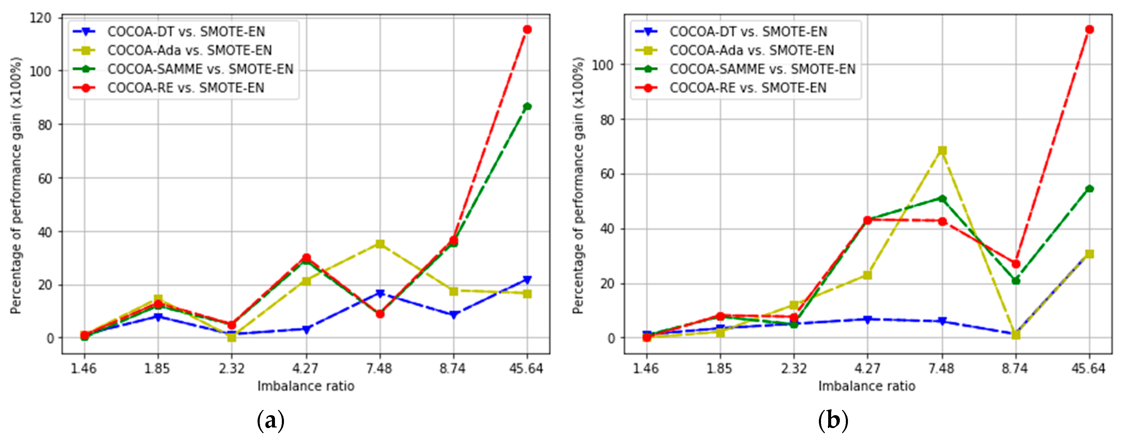
4.3. Experimental Results

Table 4 and Table 5 summarizes the detailed experimental results according to Macro-F and Macro-AUC.

Table 4. The experimental results when the binary classifier is decision tree.

Results	The Binary Classifier Is Decision Tree
	SMOTE-EN	COCOA-DT	COCOA-Ada	COCOA-SAMME	COCOA-RE
Macro-F	0.384	0.410	0.437	0.457	0.465
Macro-AUC	0.613	0.632	0.645	0.666	0.670

Note: The bold values are best among the results.

Table 5. The experimental results when the binary classifier is neural network.

Results	The Binary Classifier Is Neural Network
	SMOTE-EN	COCOA-DT	COCOA-Ada	COCOA-SAMME	COCOA-RE
Macro-F	0.392	0.412	0.441	0.464	0.477
Macro-AUC	0.620	0.646	0.654	0.660	0.671

Note: The bold values are best among the results.

For Macro-F, the results in Table 4 and Table 5 can be concluded as follows: (1) When decision tree was applied as the binary classifier, COCOA-RE significantly outperformed the comparable approach without COCOA (SMOTE-EN) by 21%. Compared to algorithms related to COCOA, COCOA-RE not only outperformed COCOA-DT that used a general (decision tree) classifier as the multi-class classifier by 13.4%, but it also outperformed the algorithms using an ensemble classifier as the multi-class classifier, such as COCOA-Ada and COCOA-SAMME. (2) When neural network was applied as the binary classifier, COCOA-RE significantly outperformed the comparable approach without COCOA (SMOTE-EN) by 21.6%. Compared to algorithms related to COCOA, COCOA-RE not only outperformed COCOA-DT that used a general classifier (neural network) as the multi-class classifier by 15.8%, but it also outperformed COCOA-Ada and COCOA-SAMME. These results illustrate that COCOA-RE is capable of achieving good balance between precision and recall in learning the class-imbalanced multi-label data set.

For Macro-AUC, the results in Table 4 and Table 5 can be concluded as follows: (1) When decision tree was applied as the binary classifier, COCOA-RE significantly outperformed the comparable approach without COCOA (SMOTE-EN) by 9.3%. Compared to algorithms related to COCOA, COCOA-RE not only outperformed COCOA-DT by 6%, but it also outperformed COCOA-Ada and COCOA-SAMME. (2) When the neural network was applied as the binary classifier, COCOA-RE significantly outperformed the comparable approach without COCOA (SMOTE-EN) by 8%. Compared to algorithms related to COCOA, COCOA-RE not only outperformed COCOA-DT that used a general classifier (neural network) as the multi-class classifier by 3.7%, but it also outperformed COCOA-Ada and COCOA-SAMME. These results demonstrate the real-value function in COCOA-RE is capable of achieving better performance than reasonable predictive confidence.

To further investigate the performance of COCOA-RE in different imbalance ratios, the performance of each approach in each class label was collected based on F-measure. In the case that algorithm A was compared with algorithm B, $A_q$ denoted the performance of algorithm A in class label $q$ and $B_q$ denoted that of algorithm B in class label $q$. The corresponding percentage of performance gain was calculated as $P{G}_q=[(A_q-B_q)/B_q]\ast 100\%$ that reflected the relative performance between algorithm A and algorithm B in class label $q$. Figure 2 demonstrates the performance gain $P{G}_q$ changes along the imbalance ratio of the class label $q$. As shown in Figure 2, irrespective of whether the binary classifier was decision tree or neural network, each algorithm based on COCOA achieved good performance against SMOTE-EN across all labels, with each $P{G}_q$ hardly coming below 0. Furthermore, the percentage of performance gain between COCOA-RE and SMOTE-EN achieved best results when the imbalance ratio was high ($\mathrm{Im}R=8.74$ and $\mathrm{Im}R=45.64$), In particular, it was larger than 100% in the case that $\mathrm{Im}R$ was equal to 45.64, which illustrates that the advantage of COCOA-RE is more pronounced when the class imbalance problem is severe in the multi-label data set.

Figure 2. Percentage of performance gain between each algorithm based Cross-Coupling Aggregation (COCOA) and SMOTE-EN ($P{G}_q$) changes along imbalance ratio of the class label $q$ : (a) the changes of performance gains based on F-measure when the binary classifier is decision tree; (b) the changes of performance gains based on F-measure when the binary classifier is neural network. SMOTE-EN: an ensemble version of synthetic minority over-sampling technique.

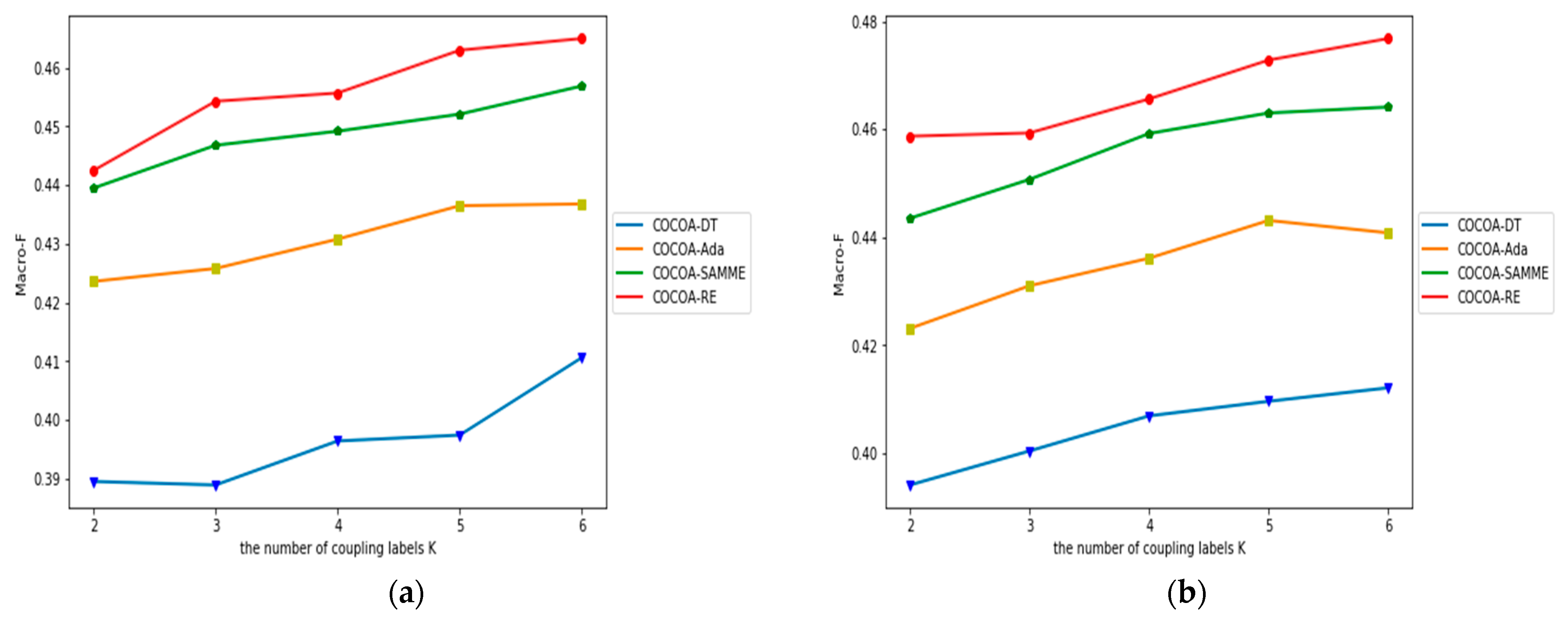
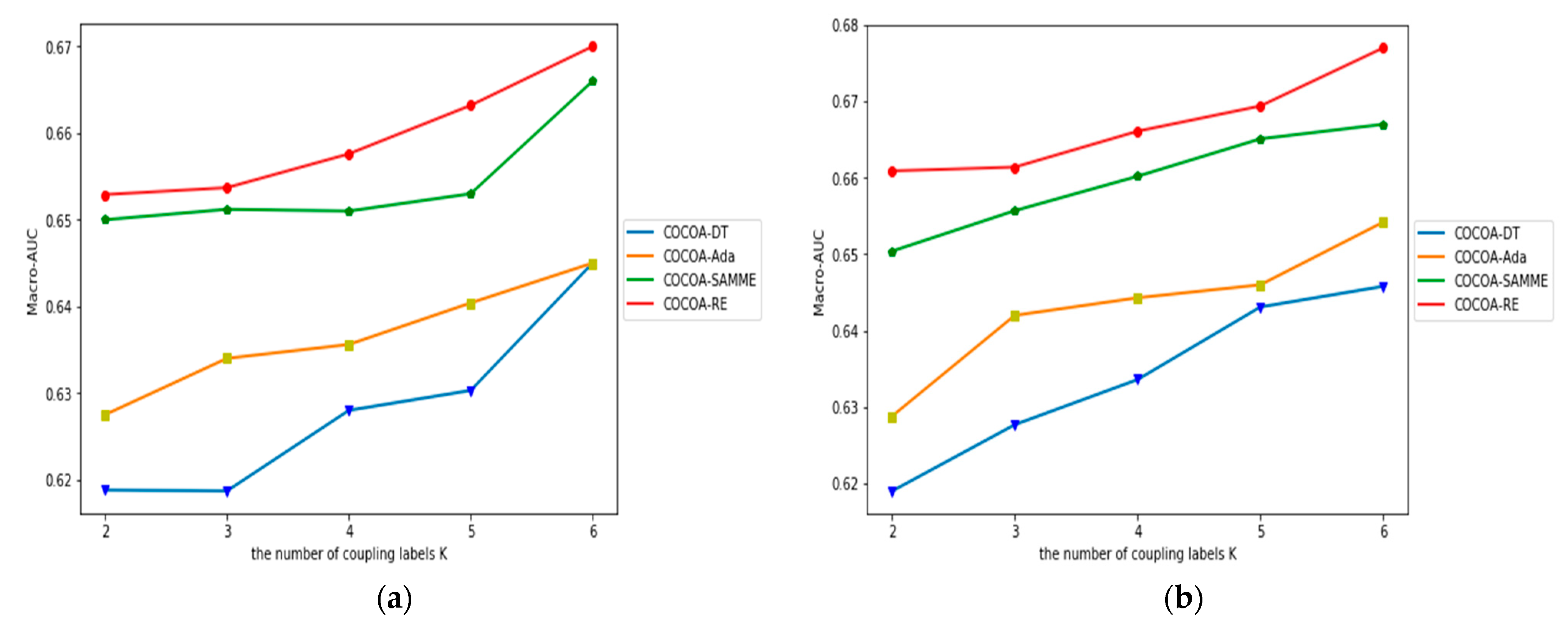
4.4. The Impact of K

To further investigate the performance of COCOA-RE in different numbers of coupling labels $K$, experiments were carried out in which $K$ was changed from 2 to 6. When Macro-F was chosen to evaluate the performance, the relative results against four comparable algorithms in which the binary classifier was decision tree is depicted in Figure 3a and that against four comparable algorithms in which the binary classifier was neural network is depicted in Figure 3b. When Macro-AUC was chosen to evaluate the performance, the relative results against four comparable algorithms in which the binary classifier was decision tree is depicted in Figure 4a and that against four comparable algorithms in which the binary classifier was neural network is depicted in Figure 4b. As shown in Figure 3 and Figure 4, COCOA-RE maintained the best performance against the comparable algorithms across different $K$ whether the evaluation metric was Macro-F or Macro-AUC. Furthermore, the COCOA-RE achieved the best Macro-F value and best Macro-AUC when the number of coupling labels $K$ was 6. These results indicate that the COCOA-RE that considers correlations between more coupling labels would achieve better performance.

Figure 3. Comparative Macro-F values with changing coupling labels: (a) the Macro-F values of different $K$ when the binary classifier is decision tree; (b) the Macro-F values of different $K$ when the binary classifier is neural network.

Figure 4. Comparative Macro-AUC values with changing coupling labels: (a) the Macro-AUC values of different $K$ when the binary classifier is decision tree; (b) the Macro-AUC values of different $K$ in the case when the binary classifier is neural network. AUC: area under the ROC curve.

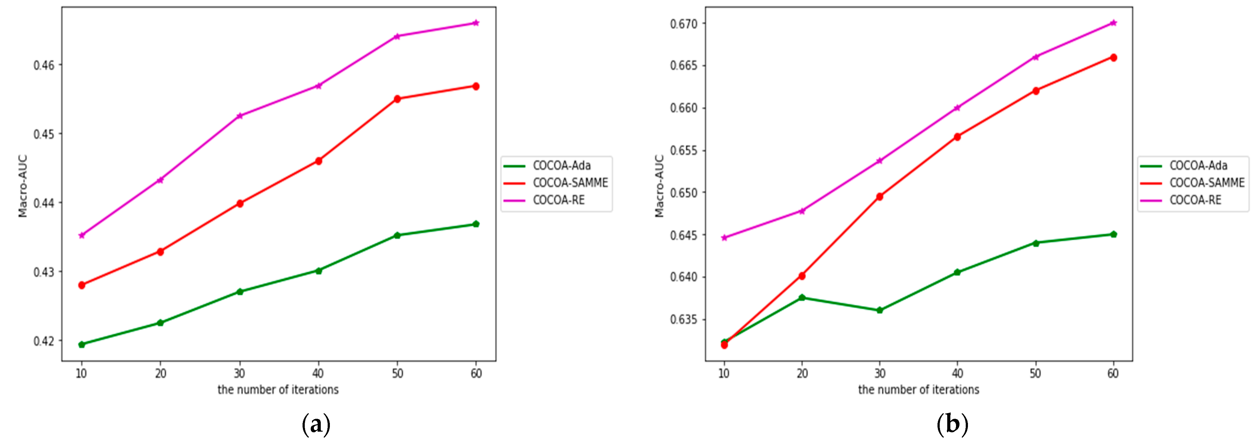
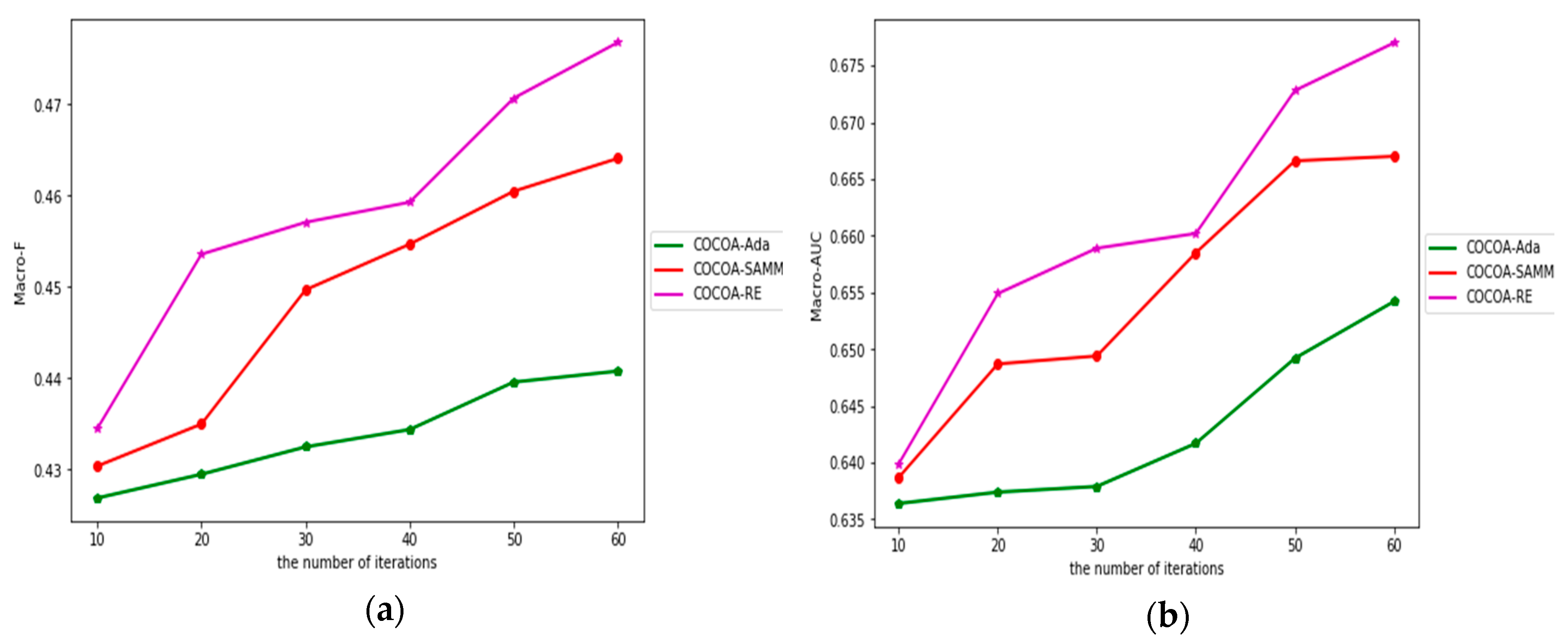
4.5. The Impact of Iterations in Ensemble Classification

It is necessary to consider the number of iterations when employing ensemble learning approaches. COCOA-Ada integrated with the ensemble algorithm named Adaboost.M1 as the multi-class classifier and COCOA-SAMME integrated with the ensemble algorithm named SAMME as the multi-class classifier were chosen to make comparisons with COCOA-RE. Using decision tree as the binary-class classifier, the Macro-F values and Macro-AUC values of comparable approaches in different iterations is shown in Figure 5a,b. Figure 6a,b present the Macro-F values and Macro-AUC values of comparable approaches in different iterations using neural network as the binary-class classifier. From these results, it can be seen that irrespective of the binary classifier chosen, COCOA-RE outperformed comparable approaches. Moreover, the Macro-F value and Macro-AUC value in COCOA-RE increased with the growth of iterations, but the rate of the increase of Macro-F value and that of Macro-AUC began slowing down when the number of iterations was higher than 50. This indicates that the performance of COCOA-RE would be improved by increasing the number of iterations. However, increasing the iterations implies that more weak classifiers are required to be trained, which would enhance the burden of computing cost. Thus, the number of iterations should not be set too large in order to avoid heavy computational cost.

Figure 5. The results with changing iterations using decision tree as the binary-class classifier: (a) the Macro-F values of comparable approaches in different iterations; (b) the Macro-AUC values of comparable approaches in different iterations.

Figure 6. The results with changing iterations using neural network as the binary-class classifier: (a) The Macro-F values of comparable approaches in different iterations; (b) the Macro-AUC values of comparable approaches in different iterations.

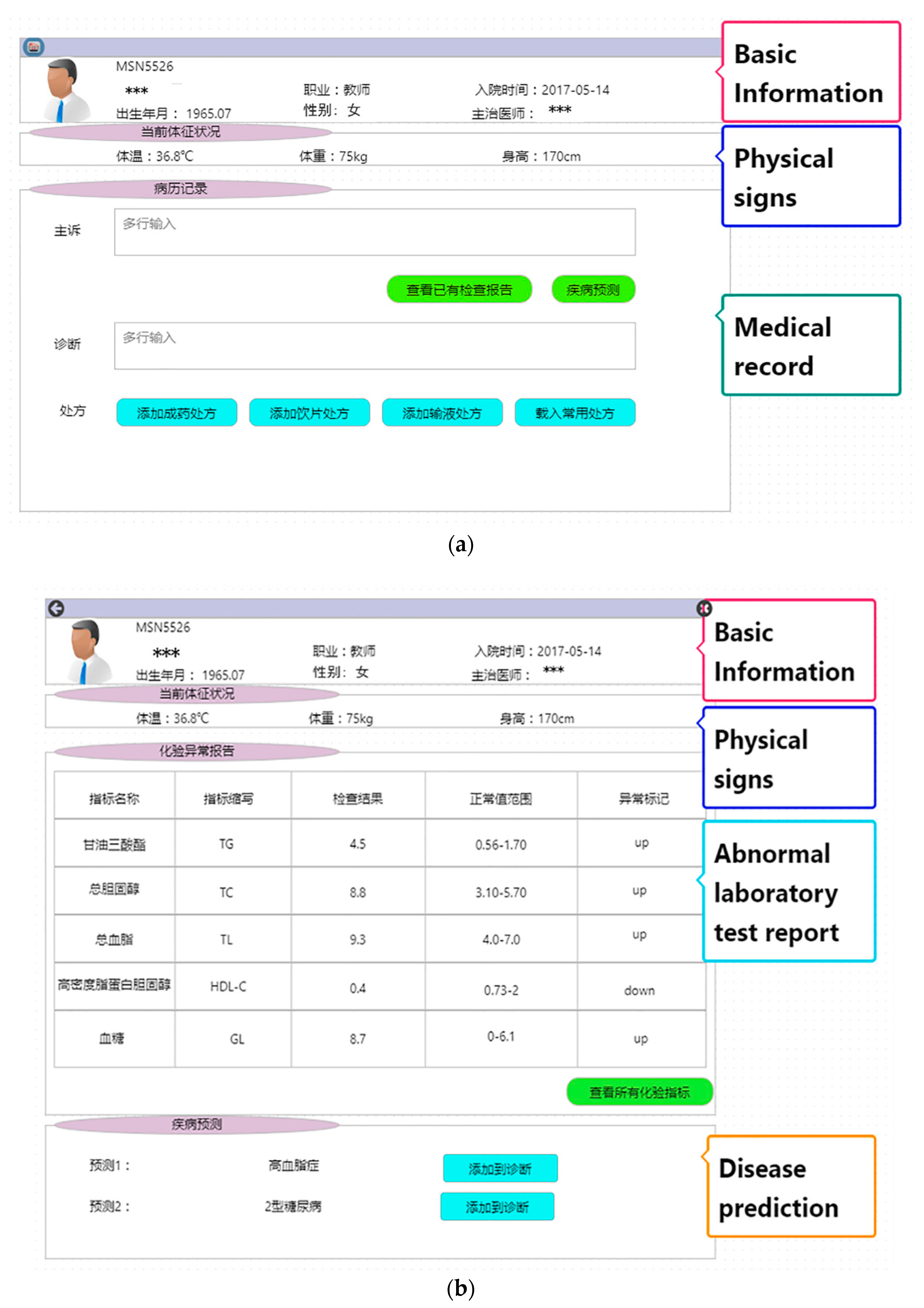
4.6. System Implementation

The proposed approach was implemented in our previously developed system prototype that can run on personal computers. A brief introduction of the developed system is given in this section. The main working interface for clinicians is described in Figure 7a, and the laboratory test report of the current patient is shown in Figure 7b. In the work interface, the pink region shows the patient’s basic information, purple region shows the patient’s physical signs, and the green region shows the patient’s medical record. In some cases, the clinician needs to review the laboratory test results before determining his or her diagnosis. The clinician can review the laboratory test report(s) (see Figure 7b) by clicking on the left green screen. In Figure 7, the blue region demonstrates the abnormal laboratory test results, and the whole laboratory test results will be shown if the green button is clicked. In terms of the predicted model train by COCOA-RE, the orange region lists one or more possible illness of the patient to the clinician. Once the clinician accepts the suggested illness, he or she can click on the “add the recommended disease to diagnosis” button (blue button) to append the recommended illness to the diagnosis automatically. After reviewing the laboratory test reports, the clinician can get back to the main work interface (Figure 7a) to continue writing the medical record for the patient by clicking the return button on the browser.

Figure 7. Two screenshots of the developed system using COCOA-RE approach: (a) the main work interface for clinicians; (b) the interface for viewing the laboratory test report.

5. Conclusions

After analyzing real-world electronic health record data, it has been revealed that a patient could be diagnosed with having more than one disease simultaneously. Therefore, to suggest a list of possible diseases, the task of classifying patients is transferred into a multi-label learning task. However, the class imbalance issue is a challenge for multi-label learning approaches. COCOA is a typical multi-label learning approach aimed at leveraging label correlation and exploring class imbalance. To improve the performance of COCOA, a regularized ensemble approach integrated into multi-class classification process of COCOA named as COCOA-RE was presented in this paper. Considering the class imbalance problem, this method leverages a regularized ensemble method to explore disease correlations and integrates the correlations among diseases in the multi-label learning process. To provide disease diagnosis, COCOA-RE learns from the available laboratory test results and essential information of patients and produces a multi-label predictive model. Experimental results validated the effectiveness of the proposed multi-label learning approach, and the proposed approach was implemented in a developed prototype system that can assist clinicians to work more efficiently.

The features extracted from laboratory test reports and essential information of patients were also considered in this paper. In our further works, features selected from more sources like textual and monitoring reports will be integrated to construct a more comprehensive profile of patients. To ensure the efficiency of the decision support system for medical diagnosis, an effective feature selection method should be used to reduce the increasing number of integrated features. In addition, multi-label approaches would process large-scale clinical data in a slow rapid, which is required to develop a more efficient multi-label learning method.

References

1. Lindmeier, C.; Brunier, A. WHO: Number of People over 60 Years Set to Double by 2050; Major Societal Changes Required. Available online: http://www.who.int/mediacentre/news/releases/2015/older-persons-day/en/ (accessed on 25 July 2018).
2. Wang, Y. Study on Clinical Decision Support Based on Electronic Health Records Data. Ph.D. Thesis, Zhejiang University, Hangzhou, China, October 2016. [Google Scholar]
3. Shah, S.M.; Batool, S.; Khan, I.; Ashraf, M.U.; Abbas, S.H.; Hussain, S.A. Feature extraction through parallel probabilistic principal component analysis for heart disease diagnosis. Phys. A Stat. Mech. Appl. 2017, 482, 796–808. [Google Scholar] [CrossRef]
4. Vancampfort, D.; Mugisha, J.; Hallgren, M.; De Hert, M.; Probst, M.; Monsieur, D.; Stubbs, B. The prevalence of diabetes mellitus type 2 in people with alcohol use disorders: A systematic review and large scale meta-analysis. Psychiatry Res. 2016, 246, 394–400. [Google Scholar] [CrossRef] [PubMed]
5. Miller, M.; Stone, N.J.; Ballantyne, C.; Bittner, V.; Criqui, M.H.; Ginsberg, H.N.; Goldberg, A.C.; Howard, W.J.; Jacobson, M.S.; Kris-Etherton, P.M.; et al. Triglycerides and Cardiovascular Disease: A Scientific Statement from the American Heart Association. Circulation 2011, 123, 2292–2333. [Google Scholar] [CrossRef] [PubMed]
6. Wang, Y.; Li, P.; Tian, Y.; Ren, J.J.; Li, J.S. A Shared Decision-Making System for Diabetes Medication Choice Utilizing Electronic Health Record Data. IEEE J. Biomed. Health Inform. 2017, 21, 1280–1287. [Google Scholar] [CrossRef] [PubMed]
7. Zhang, M.L.; Li, Y.K.; Liu, X.Y. Towards class-imbalance aware multi-label learning. In Proceedings of the Twenty-Fourth International Joint Conference on Artificial Intelligence, Buenos Aires, Argentina, 25–31 July 2015. [Google Scholar]
8. Yuan, X.; Xie, L.; Abouelenien, M. A regularized ensemble framework of deep learning for cancer detection from multi-class imbalanced training data. Pattern Recognit. 2018, 77, 160–172. [Google Scholar] [CrossRef]
9. Marco-Ruiz, L.; Pedrinaci, C.; Maldonado, J.A.; Panziera, L.; Chen, R.; Bellika, J.G. Publication, discovery and interoperability of clinical decision support systems: A linked data approach. J. Biomed. Inform. 2016, 62, 243–264. [Google Scholar] [CrossRef] [PubMed]
10. Suk, H.I.; Lee, S.W.; Shen, D. Deep ensemble learning of sparse regression models for brain disease diagnosis. Med. Image Anal. 2017, 37, 101–113. [Google Scholar] [CrossRef] [PubMed]
11. Çomak, E.; Arslan, A.; Türkoğlu, İ. A decision support system based on support vector machines for diagnosis of the heart valve diseases. Comput. Biol. Med. 2007, 37, 21–27. [Google Scholar] [CrossRef] [PubMed]
12. Molinaro, S.; Pieroni, S.; Mariani, F.; Liebman, M.N. Personalized medicine: Moving from correlation to causality in breast cancer. New Horiz. Transl. Med. 2015, 2, 59. [Google Scholar] [CrossRef]
13. Song, L.; Hsu, W.; Xu, J.; van der Schaar, M. Using Contextual Learning to Improve Diagnostic Accuracy: Application in Breast Cancer Screening. IEEE J. Biomed Health Inf. 2016, 20, 902–914. [Google Scholar] [CrossRef] [PubMed]
14. He, H.; Garcia, E.A. Learning from Imbalanced Data. IEEE Trans. Knowl. Data Eng. 2009, 21, 1263–1284. [Google Scholar] [Green Version]
15. Zhang, M.; Zhou, Z. ML-KNN: A lazy learning approach to multi-label learning. Pattern Recognit. 2007, 40, 2038–2048. [Google Scholar] [CrossRef] [Green Version]
16. Tsoumakas, G.; Katakis, I.; Taniar, D. Multi-Label Classification: An Overview. Int. J. Data Warehous. Min. 2008, 3, 1–13. [Google Scholar] [CrossRef]
17. Ghamrawi, N.; Mccallum, A. Collective multi-label classification. In Proceedings of the International Conference on Information and Knowledge Management, Bremen, Germany, 31 October–5 November 2005. [Google Scholar]
18. Elisseeff, A.; Weston, J. A kernel method for multi-labelled classification. In Proceedings of the International Conference on Neural Information Processing Systems, Vancouver, BC, Canada, 3–8 December 2001. [Google Scholar]
19. Fürnkranz, J.; Hüllermeier, E.; Mencía, E.L.; Brinker, K. Multilabel classification via calibrated label ranking. Mach. Learn. 2008, 73, 133–153. [Google Scholar] [CrossRef] [Green Version]
20. Tsoumakas, G.; Katakis, I.; Vlahavas, I. Random k-Labelsets for Multilabel Classification. IEEE Trans. Knowl. Data Eng. 2011, 23, 1079–1089. [Google Scholar] [CrossRef]
21. Tahir, M.A.; Kittler, J.; Yan, F. Inverse random under sampling for class imbalance problem and its application to multi-label classification. Pattern Recognit. 2012, 45, 3738–3750. [Google Scholar] [CrossRef]
22. Sáez, J.A.; Krawczyk, B.; Woźniak, M. Analyzing the oversampling of different classes and types of examples in multi-class imbalanced datasets. Pattern Recognit. 2016, 57, 164–178. [Google Scholar]
23. Prati, R.C.; Batista, G.E.; Silva, D.F. Class imbalance revisited: A new experimental setup to assess the performance of treatment methods. Knowl. Inf. Syst. 2015, 45, 1–24. [Google Scholar] [CrossRef]
24. Charte, F.; Rivera, A.J.; del Jesus, M.J.; Herrera, F. MLSMOTE: Approaching imbalanced multilabel learning through synthetic instance generation. Knowl.-Based Syst. 2015, 89, 385–397. [Google Scholar] [CrossRef]
25. Xioufis, E.S.; Spiliopoulou, M.; Tsoumakas, G.; Vlahavas, I. Dealing with Concept Drift and Class Imbalance in Multi-Label Stream Classification. In Proceedings of the International Joint Conference on Artificial Intelligence (IJCAI 2011), Barcelona, Spain, 16–22 July 2011. [Google Scholar]
26. Fang, M.; Xiao, Y.; Wang, C.; Xie, J. Multi-label Classification: Dealing with Imbalance by Combining Label. In Proceedings of the 26th IEEE International Conference on Tools with Artificial Intelligence, Limassol, Cyprus, 10–12 November 2014. [Google Scholar]
27. Napierala, K.; Stefanowski, J. Types of minority class examples and their influence on learning classifiers from imbalanced data. J. Intell. Inf. Syst. 2016, 46, 563–597. [Google Scholar] [CrossRef]
28. Krawczyk, B. Learning from imbalanced data: open challenges and future directions. Prog. Artif. Intell. 2016, 5, 1–12. [Google Scholar] [CrossRef]
29. Guo, H.; Li, Y.; Li, Y.; Liu, X.; Li, J. BPSO-Adaboost-KNN ensemble learning algorithm for multi-class imbalanced data classification. Eng. Appl. Artif. Intell. 2016, 49, 176–193. [Google Scholar]
30. Cao, Q.; Wang, S.Z. Applying Over-sampling Technique Based on Data Density and Cost-sensitive SVM to Imbalanced Learning. In Proceedings of the 2012 International Joint Conference on Neural Networks (IJCNN), Brisbane, Australia, 10–15 June 2012. [Google Scholar]
31. Fernández, A.; López, V.; Galar, M.; Jesus, M.J.; Herrera, F. Analyzing the classification of imbalanced data-sets with multiple classes: Binarization techniques and ad-hoc approaches. Knowl.-Based Syst. 2013, 42, 91–100. [Google Scholar]
32. Freund, Y.; Schapire, R.E. A desicion-theoretic generalization of on-line learning and an application to boosting. J. Comput. Syst. Sci. 1997, 13, 663–671. [Google Scholar]
33. Schapire, R.E.; Singer, Y. Improved Boosting Algorithms Using Confidence-rated Predictions. Mach. Learn. 1999, 37, 297–336. [Google Scholar] [CrossRef] [Green Version]
34. Zhu, J.; Zou, H.; Rosset, S.; Hastie, T. Multi-class AdaBoost. Stat. Interface 2009, 2, 349–360. [Google Scholar] [Green Version]
35. Chawla, N.V.; Bowyer, K.W.; Hall, L.O.; Kegelmeyer, W.P. SMOTE: Synthetic minority over-sampling technique. J. Artif. Intell. Res. 2002, 16, 321–357. [Google Scholar] [CrossRef]
36. López, V.; Fernández, A.; García, S.; Palade, P.; Herrera, F. An insight into classification with imbalanced data: Empirical results and current trends on using data intrinsic characteristics. Inform. Sci. 2013, 250, 113–141. [Google Scholar]
37. Zhang, M.L.; Zhou, Z.H. A Review on Multi-Label Learning Algorithms. IEEE Trans. Knowl. Data Eng. 2014, 26, 1819–1837. [Google Scholar] [CrossRef]