A Fusion Feature Extraction Method Using EEMD and Correlation Coefficient Analysis for Bearing Fault Diagnosis


1
School of Mechatronic Engineering, China University of Mining and Technology, Xuzhou 221116, China
2
Jiangsu Key Laboratory of Mine Mechanical and Electrical Equipment, China University of Mining and Technology, Xuzhou 221116, China
*
Author to whom correspondence should be addressed.
Appl. Sci. 2018, 8(9), 1621; https://doi.org/10.3390/app8091621
Submission received: 14 August 2018
/
Revised: 4 September 2018
/
Accepted: 10 September 2018
/
Published: 12 September 2018
(This article belongs to the Special Issue Fault Detection and Diagnosis in Mechatronics Systems)
Abstract
:Acceleration sensors are frequently applied to collect vibration signals for bearing fault diagnosis. To fully use these vibration signals of multi-sensors, this paper proposes a new approach to fuse multi-sensor information for bearing fault diagnosis by using ensemble empirical mode decomposition (EEMD), correlation coefficient analysis, and support vector machine (SVM). First, EEMD is applied to decompose the vibration signal into a set of intrinsic mode functions (IMFs), and a correlation coefficient ratio factor (CCRF) is defined to select sensitive IMFs to reconstruct new vibration signals for further feature fusion analysis. Second, an original feature space is constructed from the reconstructed signal. Afterwards, weights are assigned by correlation coefficients among the vibration signals of the considered multi-sensors, and the so-called fused features are extracted by the obtained weights and original feature space. Finally, a trained SVM is employed as the classifier for bearing fault diagnosis. The diagnosis results of the original vibration signals, the first IMF, the proposed reconstruction signal, and the proposed method are 73.33%, 74.17%, 95.83% and 100%, respectively. Therefore, the experiments show that the proposed method has the highest diagnostic accuracy, and it can be regarded as a new way to improve diagnosis results for bearings.
1. Introduction
Rolling element bearings are commonly employed to support rotating shafts in a rotary machine. A bearing mainly includes an inner race, an outer race, and several rolling elements. A fault in any one of the above-mentioned components can result in the reduced performance of the whole system, fatal machine failure, or catastrophic accident [1,2,3]. Based on the statistical results in Ref. [4], more than 50% of mechanical faults are caused by various bearing defects. Therefore, it is important and necessary to design a effective solution for bearing fault diagnosis to reduce the loss caused by mechanical failure.
Analyzing different features extracted from vibration signals has been testified to play an exceptionally effective role in addressing the issue of fault detection or fault diagnosis of rotary machinery, because these obtained vibration signals provide abundant information regarding the working conditions of the bearings in a rotary machine [5,6]. Up to now, many signal processing methods have been employed to analyze the collected vibration signal for features, and they can be summed into three types: time domain, frequency domain, and time-frequency domain [7]. At the preliminary stage of mechanical fault diagnosis, time domain analysis is the simplest one. Frequency domain methods typically diagnose mechanical faults by revealing key frequency information regarding faults, for example, fast Fourier transform (FFT) [8] and interpolated discrete Fourier transform (IpDFT) [9]. However, the above two methods alone can only extract a portion of the useful information from the vibration signals, and information from each of the other domains is lost. Therefore, more and more researchers have introduced time-frequency processing tools for mechanical feature extraction, such as short-time Fourier transform (STFT), wavelet transform-based methods, empirical mode decomposition (EMD), and ensemble empirical mode decomposition (EEMD) [10,11,12,13]. As a self-adaptive signal processing algorithm, EMD can analyze the overlap information in both time and frequency domains [14]. Therefore, many EMD-based methods have been proposed for mechanical fault diagnosis. A fault diagnosis method was employed using envelope spectrum analysis with the EMD algorithm in Ref. [15]. Wu and Qu [16] proposed an effective method to search the features of subharmonic faults of large rotating machinery based on EMD; this is an adaptive and unsupervised approach that does not require a shift to the frequency domain.
In Ref. [17], a novel method combining the parameter estimate of Alpha stable distribution (ASD) and EMD-based signal processing was proposed to diagnose low-speed bearing faults. In this method, the trend and noise components of the vibration signal were filtered to give a clear signal. An accurate autoregressive (AR) model can reveal important information or characteristics of a dynamic system, so this model was combined with EMD to construct a new strategy to extract effective features for bearing fault diagnosis [18]. In [19], a new fault diagnosis method using EMD and wavelet denoising analysis was designed for bearing systems. However, traditional EMD can suffer from a mode-mixing problem when used to analyze complex signals. To settle the mode-mixing issue, an improved version, called EEMD, was designed by Wu and Huang [20]. A multi-fault diagnosis method for axle bearings was introduced using EEMD and Hilbert marginal spectrum analysis [21]. In this method, an intrinsic mode function (IMF) confidence index was designed to realize the aim of adaptive self-selection of the useful IMFs. In Ref. [22], EEMD and multi-scale fuzzy entropy were introduced for feature extraction from complex vibration signals, and this method was also used for motor bearing fault diagnosis. Another effective fault diagnosis method uses improved EEMD and Hilbert square demodulation (HSD) [23]. The fault feature information of weak faults is difficult to extract directly using the standard EEMD algorithm; hence, Wang et al. [24] proposed a novel feature extraction strategy to detect bearing weak faults based on tunable Q-factor wavelet transform and traditional EEMD. Similarly, Yang et al. [25] used EEMD and correlation coefficients to extract effective features by adaptive denoising analysis. In addition to the above studies, a discussion of other EEMD-based fault diagnosis methods can be found in Refs. [26,27,28].
Feature extraction is one step towards obtaining useful information regarding mechanical faults. A classifier must then be designed to complete the process of mechanical fault diagnosis. Many intelligent classification approaches have been presented for mechanical fault diagnosis. Li et al. [29] introduced artificial neural networks (ANN) to diagnose the gearbox faults of a marine propulsion system using the bi-spectrum technique. Chen et al. Ref. [30] used Bayesian networks for the fault diagnosis of a wind turbine gearbox. In Ref. [31], fuzzy inference was employed to diagnose early bearing faults with morphological operators. In addition, other neural network-based methods were developed for mechanical fault diagnosis in Refs. [32,33]. There are disadvantages of ANNs and drawbacks to back-propagation (BP) or radial basis function (RBF)-based fault diagnosis methods. For example, obvious over-fitting, low convergence rate, and especially poor generalization will appear if the number of the used training samples is small [34]. Therefore, support vector machine (SVM) was introduced as a new classifier to diagnose mechanical faults. SVM techniques are easier to use and address nonlinearity classification problems. Therefore, numerous SVM-based mechanical fault diagnosis strategies have been proposed [35,36,37].
In this paper, a new approach to information fusion is proposed for bearing fault diagnosis which fully uses the vibration signals of multi-sensors. Although this method is based on traditional tools, such as EEMD, SVM, and correlation coefficient analysis, a correlation coefficient ratio factor (CCRF) is defined to select sensitive IMFs to reconstruct new vibration signals for further feature fusion analysis, and a new weight computation strategy is designed to fuse these features of multi-sensors. First, EEMD is applied to decompose the vibration signal into a set of intrinsic mode functions (IMFs) and the so-called CCRF is defined to select sensitive IMFs, and a new reconstructed vibration signal is obtained. Second, an original feature space is constructed from the reconstructed signal. Afterwards, weights are assigned by correlation coefficients among the vibration signals of considered multi-sensors, and the so-called fused features are extracted by the obtained weights and original feature space. Finally, a trained SVM is employed as the classifier for bearing fault diagnosis.
Other parts of this paper are arranged as follows. The theoretical background, including the principles of EMD, EEMD, and SVM, are introduced in Section 2. Section 3 shows the proposed method, which includes sensitive IMF selection with the correlation coefficient ratio factor (CCRF), the feature fusion principle of multiple sensors, and fault diagnosis based on SVM. In Section 4, experimental research is performed on a multi-function mechanical fault simulator. The conclusions of this work are made in Section 5.
2. Theoretical Background
2.1. EMD Theory
EMD is a time-frequency analysis method and can self-adaptively process complex signals into a set of IMFs. It works with three assumptions [14]: (1) the target signal must have at least two extrema (one maximum and one minimum); (2) the characteristic time scale is defined by the time lapse between the extrema; and (3) if the data are totally devoid of extrema but contain only inflection points, then they can be differentiated one or more times to reveal the extrema. In addition, the obtained IMFs of EMD are nearly orthogonal functions and simple oscillation modes with physical significance. The procedure of EMD is shown as follows [14,15,16,17,18,19].
(1) Use the cubic spline line to produce upper and lower envelopes with all the local extrema points of the original signal ().
(2) Define the mean of the obtained upper and lower envelopes as , and then calculate the difference between and by
Here, there are two standards that should be used to judge whether is a strict IMF [14]. If satisfies the above two standards, then it is regarded as the first IMF component; otherwise, is treated as , and steps (1) and (2) are repeated n times until is a real IMF. As a result, the first IMF can be obtained by
(3) Then, we can obtain
where is named the residue.
Repeat above steps K times when is monotonous or the program meets the stop condition. Then, we can obtain the total K IMFs and satisfy
Finally, is decomposed into
2.2. EEMD Theory
The traditional EMD method has a mode-mixing problem when it is employed to analyze complicated vibration signals. To prevent this issue, an improved version, called EEMD, was proposed by Wu and Huang based on EMD in 2009 [20]. The fundamental basis of EEMD adaptively decomposing complicated signal signals are the added noise can make the impact interference smoother than that in original vibration signal; and the added noise components in an IMF can be canceled by averaging a set number of IMFs in several decomposition processes, because white noise has the properties of zero mean and consistency distribution in the time domain. That is to say, traditional EEMD mainly includes two parts that involve adding the appropriate noise; processing the noise-added signals with EMD several times; and then calculating the mean values of obtained IMFs. The main steps of EEMD are shown below [20,21,22,23].
(1) Determine the decomposition number (N) and add the noise amplitude (A).
(2) Generate a white noise with amplitude A, and add it to as
where is the added white noise.
(3) Employ the traditional EMD to process above noise-added signal to get
where and are the m-th IMF signal and residual signal of the n-th EMD decomposition.
(4) Repeat steps (1) to (3) N times and each time, where the added noise signals are different, their amplitudes are all equal to A.
(5) The final IMFs can be expressed as
(6) Final, the original vibration signal is decomposed into
2.3. SVM Theory
Based on the structural risk minimization principle and statistical learning theory, SVM was presented to deal with regression analysis and regression analysis issues. This algorithm can achieve the best combination of learning precision and identification accuracy with only a few samples [38]. SVM is mainly to construct a classification hyperplane to separate the data points of two classes and to maximize the margin of separation hyperplane between these two data sets. When SVM is used as a classifier, it firstly projects input data into the high dimension space by the way of nonlinear transformation, and then an optimal hyperplane is found to classify input data sets. Therefore, the construction of the SVM-based classifier can be treated as a quadratic optimization issue. The generalization ability of SVM is stronger than traditional nonlinear function approximation algorithms. At the same time, SVM can overcome the difficulty in determining the network structure and local minima of the neural network. Therefore, SVM has advantages in the classification of small sample sets and pattern recognition of high dimensional data sets. The principles of SVM are briefly described below [35,36,37,38,39].
Set the training sample dataset to (,), , , (1, −1). These samples can be classified by a hyperplane which is described as
where w denotes the n dimensional weight vector which is perpendicular to the hyperplane, and b is a scalar. If we get a perpendicular, it can be classified by the sample dataset with
To reduce the classification error of the SVM model, the optimization values of w and b should be found to make the separating margin maximum. That is to say, the SVM-based classification finally become a quadratic optimization problem. In practical applications of SVM, the sample data set is usual a nonlinearly separable, and the samples should be mapped to high dimensional space with the kernel function before doing the classification.
3. Proposed Method
3.1. Sensitive IMF Selection
According to the principles of EEMD, a series of IMFs can be obtained when using it to deal with the complex signal. Simultaneously, the so-called useful information regarding mechanical faults is assigned to various IMF components. Therefore, how to select the sensitive decomposed composition is important for constructing a precise fault diagnosis method. Up to now, two common ways have been kurtosis analysis [40] and correlation analysis [41]. For the former, the first IMF has the biggest kurtosis because of the interference of noise and the high frequency component. For the latter, only the correlations of IMFs between observational vibration signal of are use, but the correlations of IMFs between the vibration signal of normal are not considered. Here, we combine above two types of correlations to select sensitive IMFs, and the main steps are shown below.
(1) Set and as the vibration signals of normal bearing and investigated bearing conditions, respectively. Then, compute the correlation coefficient of the ith IMF and by
where is the ith decomposed IMF of EEMD; and are the deviations of and , respectively; and are the means of and .
(2) Compute the correlation coefficient () between the vibration signal under normal conditions and the ith IMF with Equation (12).
(3) Calculate the ratio between and using
where is defined as the correlation coefficient ratio factor (CCRF) that is used to select sensitive IMFs.
(4) Rank these CCRF values as a new sequence from biggest to smallest, i.e., , and M represents the total number of CCRFs.
(5) Select K IMFs with the larger CCRF values and assign the weight, , to the kth selected sensitive IMF. Then, a new reconstructed signal is obtained by
The two correlation coefficients calculated in steps (1) and (2) reflect the correlation degrees of these decomposed IMFs with their original vibration signals and . In accordance with the similarity theory, and are between zero and one. If the correlation coefficient is equal to zero, these two signals are completely uncorrelated. If the correlation coefficient is equal to one, these two signals are completely correlated. That is, the larger is, the more related the ith IMF and will be; the smaller is, the less related the ith IMF and will be. From Equation (13), it can be observed that considers not only the value of but also the ratios of and . Therefore, we can select the components with the greatest CCRF values as the sensitive IMFs. In this paper, three sensitive IMFs were obtained for further feature extraction analysis.
3.2. Feature Fusion of Multiple Sensors
For a rotating machine, several vibration signals can be collected by sensors installed at different locations on the machinery, and many parameter values can also be calculated as the features from the vibration signal collected by each sensor. Using the proposed sensitive IMF selection method, the useful information from each sensor for fault diagnosis is obtained, and traditional features are extracted. If all features are employed to diagnose bearing faults, the fault diagnosis model will be complicated and time-consuming. Furthermore, each feature can contain more or less failure information to facilitate the fault diagnosis of the bearings. Principal component analysis (PCA) can play a role in projecting high-dimensional data to low-dimensional data to reduce the redundancy of the dataset [42]. Meanwhile, the low-dimensional data is able to reflect the main information of the original high-dimensional data. However, one drawback of PCA is that its threshold is hard to adaptively select. Another frequently used feature fusion method is the DS evidence theory [43], which has become a more widely used approach in recent years. However, it also has problems. For example, the exponential complexity of the computations and fusing of conflicting data can produce counterintuitive results [44]. In this paper, we use correlation analysis to fuse these obtained features from different sensors. The procedure is as follows.
(1) The reconstructed signals with selected sensitive IMFs of the used sensors are obtained using the sensitive IMF selection method described in Section 3.1; these are marked as , …, where sn is the serial number of the sensor.
(2) The characteristic parameter values are calculated from the reconstructed signals of the sensors with the definitions and calculated formulas of the features.
(3) The correlation coefficients of any two reconstructed signals are calculated and the two reconstructed signals, and , with the greatest correlation coefficients are determined. For normal conditions, either of these two reconstructed signals, or , can be selected as the base signal. For the investigated vibration signal, this reconstructed signal, which has the lowest correlation with the normal signal, is regarded as the so-called base signal. Then, the correlation coefficients of the base signal and all reconstructed signals are calculated to define a weight, , by
where is the correlation coefficient of the base signal and reconstructed signals; is the base signal; and is the reconstructed signal and can be equal to .
(4) After obtaining these weights, the fusion features are calculated by
where is the original feature and is the fusion feature.
3.3. Procedure of the Proposed Method
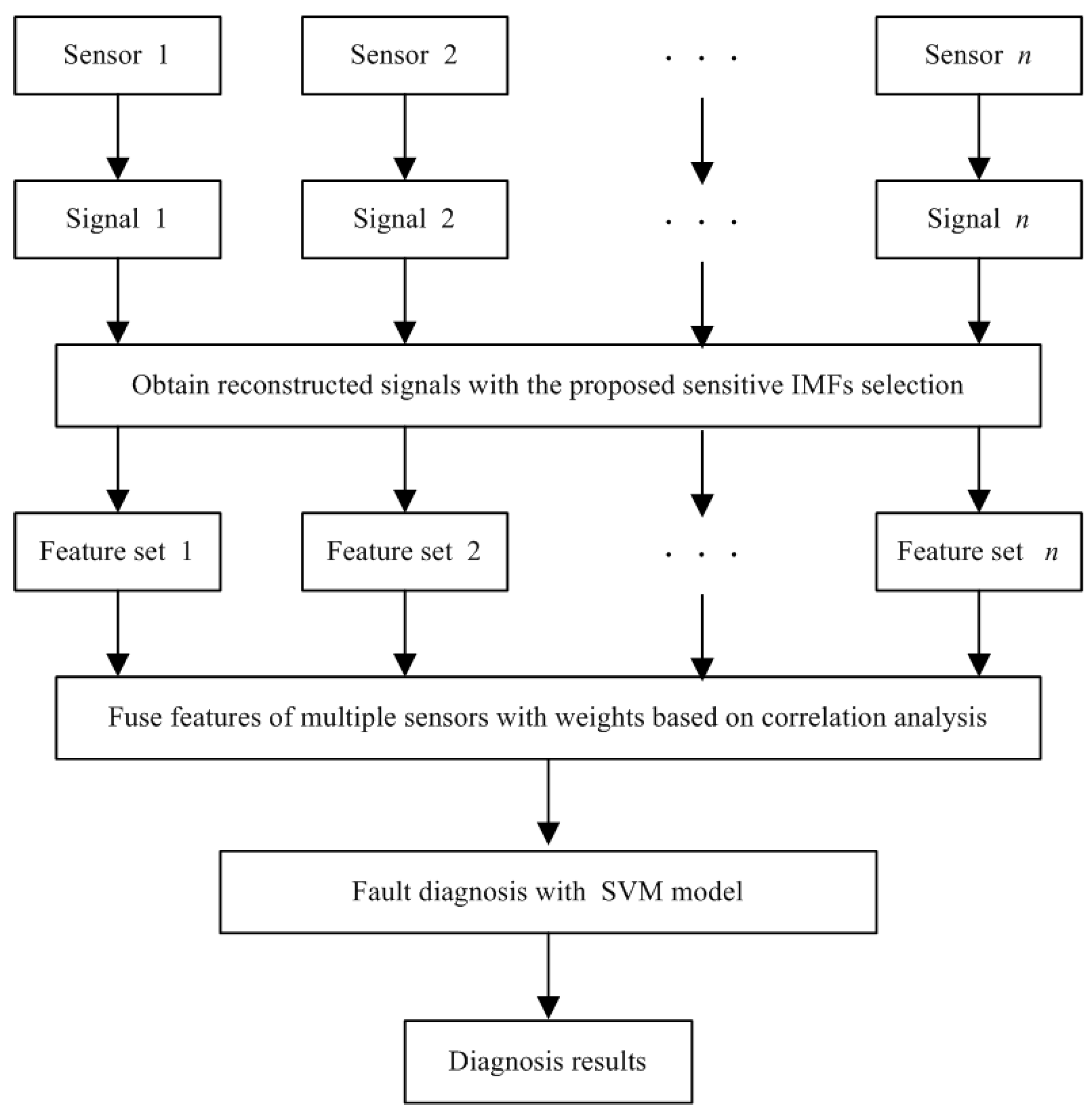
The essence of mechanical fault diagnosis is a pattern recognition problem and includes data acquisition, feature extraction, and fault classification. In the past, vibration signals have been widely used for the fault diagnosis of machines. In this paper, the vibration signals of multi-sensors are also used for bearing fault diagnosis, and the main procedure of the presented method is plotted in Figure 1.
Step 1: Install the considered acceleration sensors on the bearing housing, for example, on the top or sides. Then, vibration signals are collected by multi-sensors and the data acquisition system. In this paper, they are all bought from professional data collection companies to make the signals accurate and effective.
Step 2: The traditional EEMD algorithm is used to decompose the collected vibration signals into a set of IMFs. For this task, it is carried out offline in this paper, because a lot of computation time is need to decompose many data segments to extract features to train the SVM model.
Step 3: The proposed sensitive IMFs selection method is applied to find useful IMFs which include abundant fault information to reconstruct a new vibration signal. Then, an original feature space including features in a time domain and frequency domain is produced from the reconstructed signal. For each sensor, there is a original feature space.
Step 4: The proposed feature fusion method is performed. Here, weights are assigned by the principle defined in Section 3.2, and the so-called fused features are extracted by the obtained weights and original feature space.
Step 5: Part fusion features are randomly selected to train the standard SVM model to construct a classifier for bearing fault diagnosis, and the rest of these fusion features are used to test the proposed method.
4. Experiment
4.1. Experimental Setting
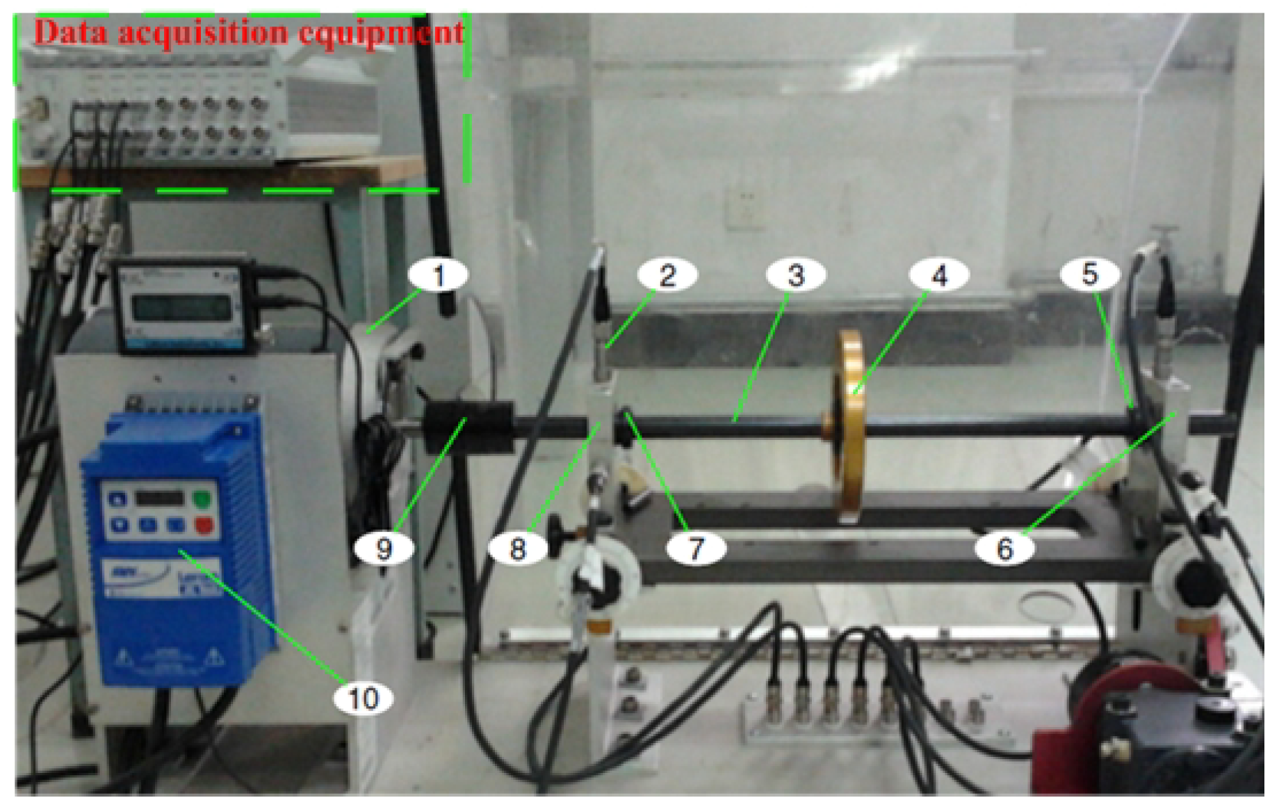
In this section, an experiment was designed on a mechanical simulator to testify the proposed method. The used simulator was produced by Spectra Quest, Inc. (Richmond, VA, USA). and is illustrated in Figure 2. This simulator is driven by a 1 Hp AC motor, and its speed can range from 0 to 6000 rpm through the control of the matched converter. The power of the motor is transmitted to the shaft through a flexible coupling, and then the bearings and well-balanced rotor disc are driven. To realize the function of increasing the rotor weight and simulating an unbalanced fault, several tapped holes are symmetrically arranged in the edge of the rotor. The above mechanical parts include several accessories, both those that function normally and those with different faults. According to the literature [45], one of the key factors affecting mechanical running states is bearing detection. Therefore, only faulty bearings were installed in this test bench to simulate the different bearing working conditions to verify the proposed method. From Figure 2, we can also see that there are two housings: the one near the AC motor is defined as inboard bearing housing and the one far from the AC motor is named outboard bearing housing. The extreme case of simultaneous failure of both bearings was not considered in this paper, so only this bearing in outboard bearing housing was defined as the test bearing, and the other one was defined as normal bearing. Some key technical characteristics are shown in Table 1. Moreover, the test bench also includes a loading system; however, all of our simulations were performed under a no loading condition.
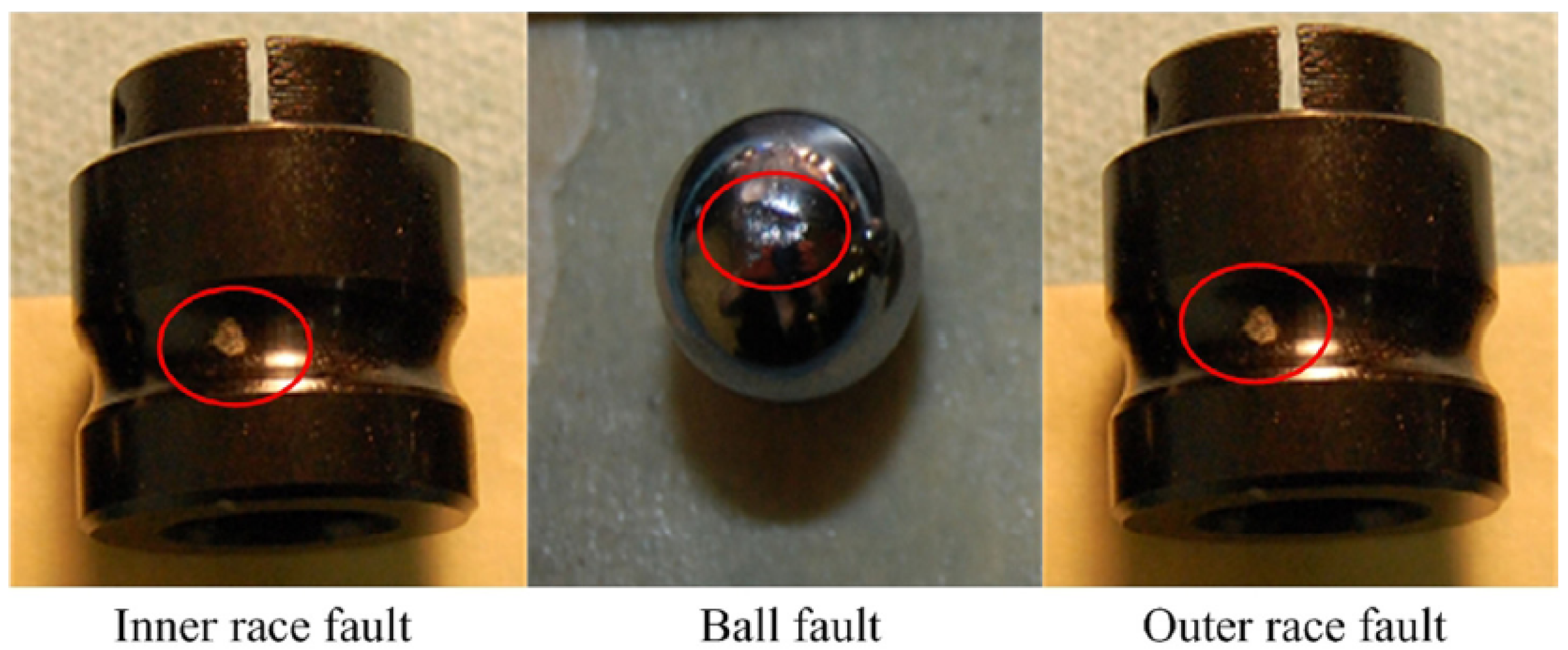
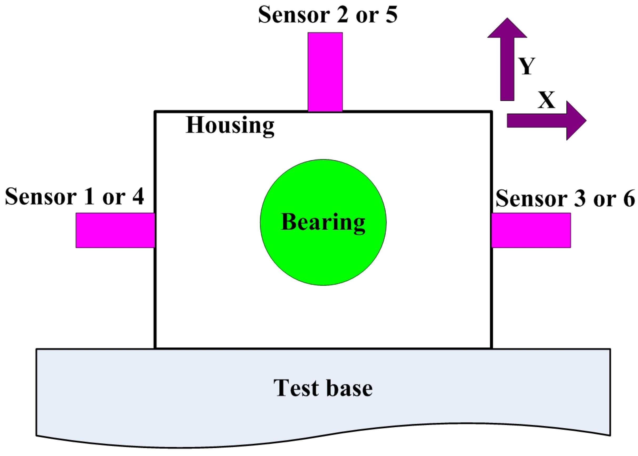
For a bearing, its faults are usually appear in inner race, outer race, and rolling elements. Considering this, four bearing working states were set: normal (S1), inter-race fault (S2), ball fault (S3), and outer-race fault (S4). These above faults were artificially processed and are shown in Figure 3. To make the simulated faults as real as possible, the diameter and depths of these faults were 2 and 0.5 mm, respectively. When the vibration signal passed to the sensor, each intermediate transmission unit caused information loss. That is to say, the more the intermediate transmission units existed, the more the loss of information would be. Based on this issue, three ICP acceleration sensors (AC 240-1D), bought from the Connection Technology Center, Inc. (New York, NY, USA), were placed on each bearing housing, and they are shown in Figure 4. For each housing, two sensors, installed on the sides, were all in the X axis; the other one, installed on the top of housing, was in the Y axis. Therefore, a total of six identical sensors were considered in this work. In addition, data acquisition equipment, produced by Donghua Testing Technology Co., Ltd. (Jingjiang, China), was also used to collected vibration signals. This device has 16 channel data recorders and can collect signals from 16 sensors at the same time. Even though the max sampling frequency of each recorder is up to 256 kHz, the real used sampling frequency is only 2 kHz by considering that the rotational speed is 1800 rpm and main fault character frequencies are less than 1 kHz.
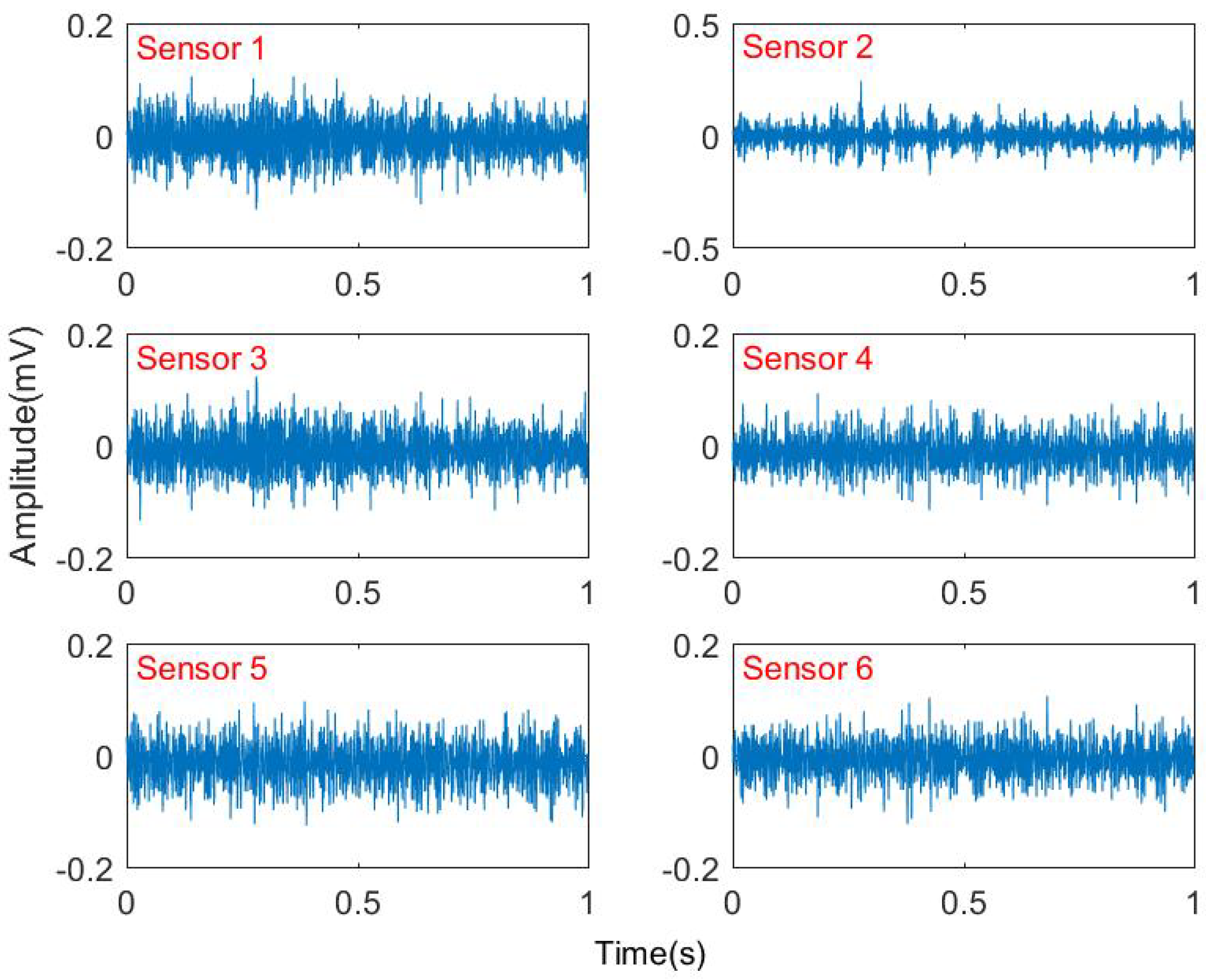
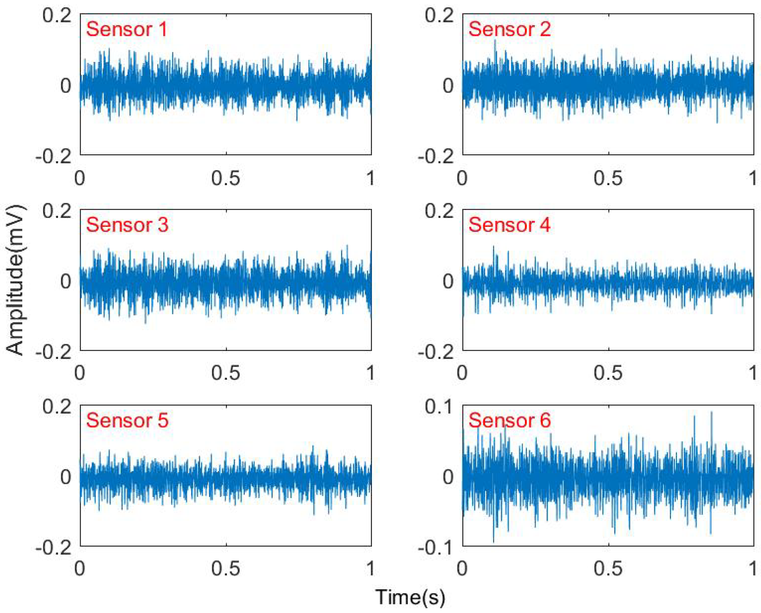
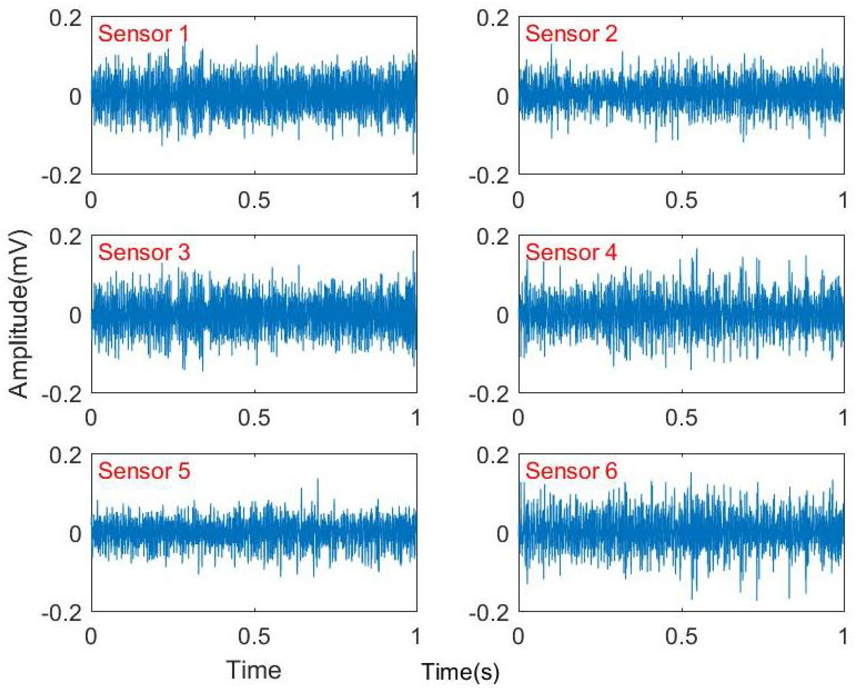
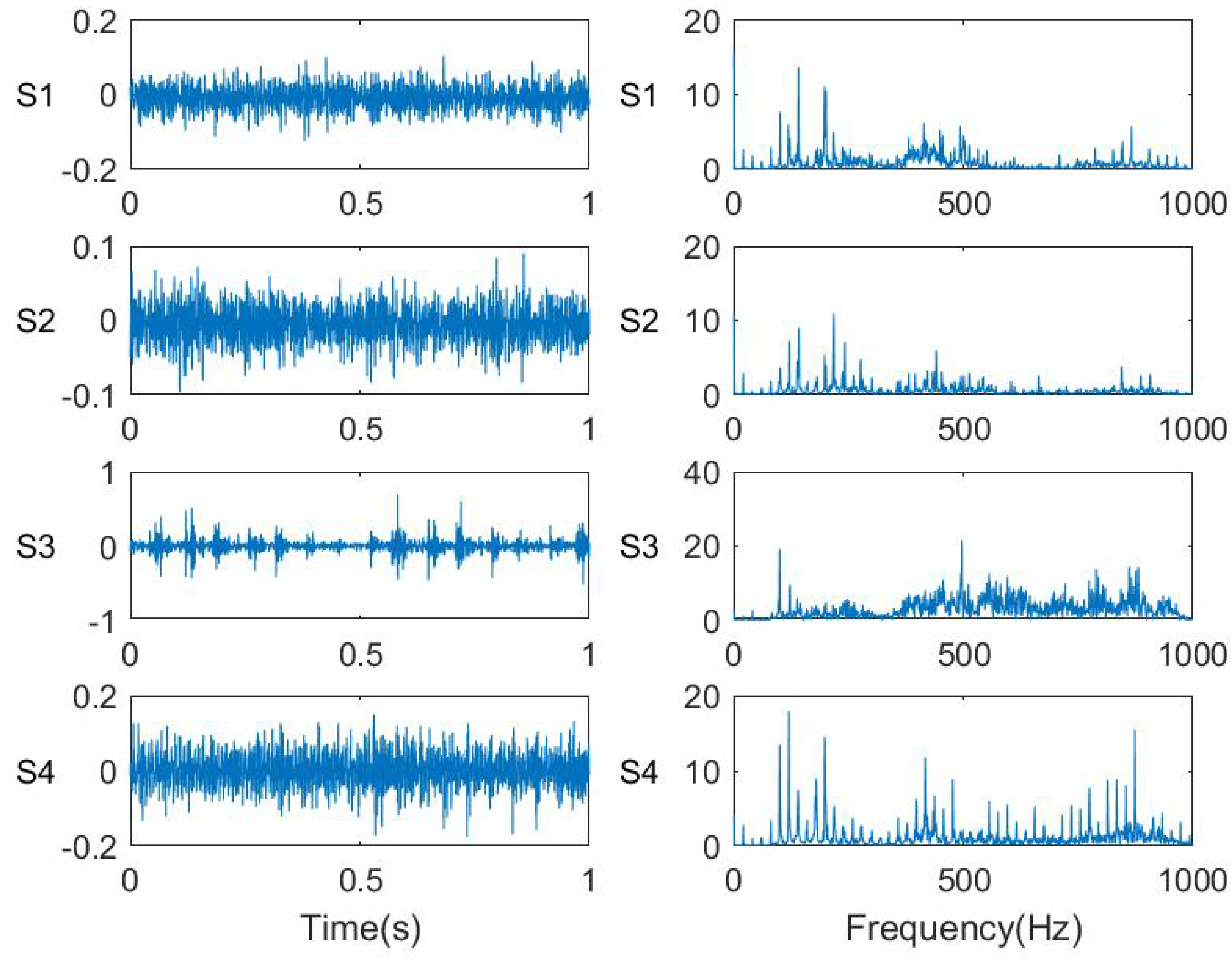
Figure 5, Figure 6, Figure 7 and Figure 8 illustrate the vibration signals of the six sensors installed on the above simulator. To optimize the layout and structure of this paper, here, only the spectrums of vibration signals collected by Sensor 6 are displayed in Figure 9. From these plots shown in Figure 5, Figure 6, Figure 7, Figure 8 and Figure 9, it can be seen that these time domain signals of various bearing states do not have enough obvious differences for fault diagnosis; similarly, it is also hard to use the differences between frequency signals for bearing fault diagnosis. That is, it is difficult to diagnose bearing faults only using these time signals or frequency signals, so their features should be extracted to finish the bearing fault diagnosis.
4.2. Fusion Feature Extraction Based on Sensitive IMF Selection
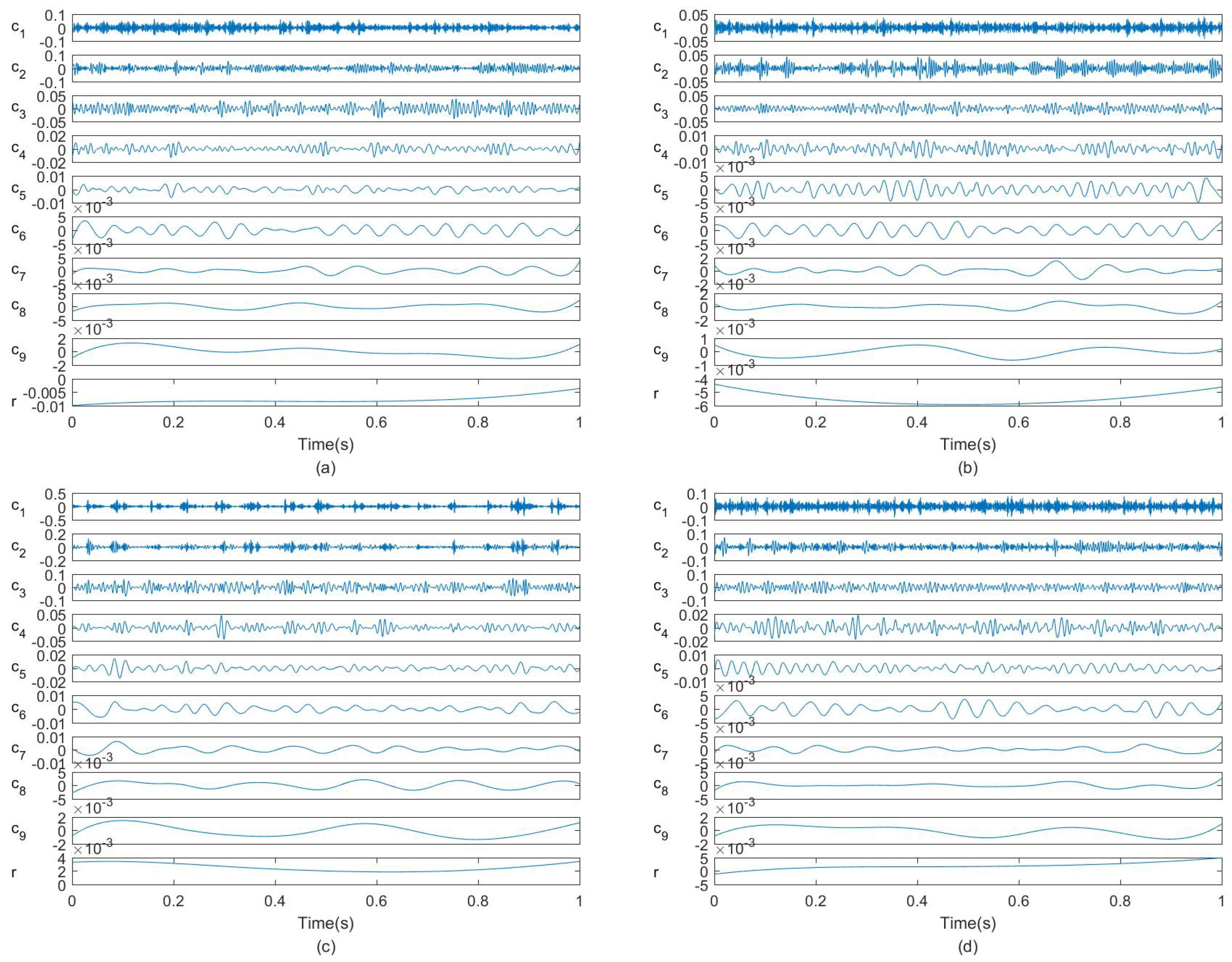
In this work, EEMD was used to deal with these obtained vibration signals. In this process, the decomposition number and amplitude of the added white noise were set as 100 and 0.2 times the standard deviation of the original signal. Figure 10 displays the decomposed IMFs of these vibration signals collected by Sensor 6 under conditions S1, S2, S3, and S4, mentioned above. When analysing these waves in Figure 10, it can be observed that the high frequency information mainly occupies the first several IMFs and the last several IMFs contain less useful low frequency information. Therefore, it was necessary to develop an adaptive sensitive IMF evaluation method.
The CCRF values of the IMFs plotted in Figure 10 were calculated and are presented in Table 2 as a digital representation. From this table, it can be observed, from the CCRF values, that the most sensitive IMFs are the first several IMFs of EEMD. That is, the last IMFs are of minimal value for fault diagnosis and can be removed as noise. The CCRF values in Table 2 indicate that the most sensitive IMFs are the first several IMFs of EEMD. In this paper, the first three IMFs with the greatest CCRF values were selected to reconstruct the vibration signals for the features. The reconstructed vibration signals of Sensors 1–6 were calculated using Equation (14). Then, the original features, identified in Ref. [46], were calculated for fusion features calculated by correlation analysis and weighted average. Table 3 displays the group weight values of the six sensors under the four considered conditions. From this table, it can be observed that the weights belonging to the six sensors were different in value; the greatest weight values belonged to Sensor 1 (once) and Sensor 3 (three times). Therefore, using a traditional averaging method to fuse the features of the six sensors would ignore the contributions of the original features. That is, the features with more useful information and the features with less useful information would contribute the same weighting when calculating the fusion features using a traditional averaging method. To fully use the pertinent information of the six sensors, fusion features were extracted using Equation (16).
4.3. Results and Discussion
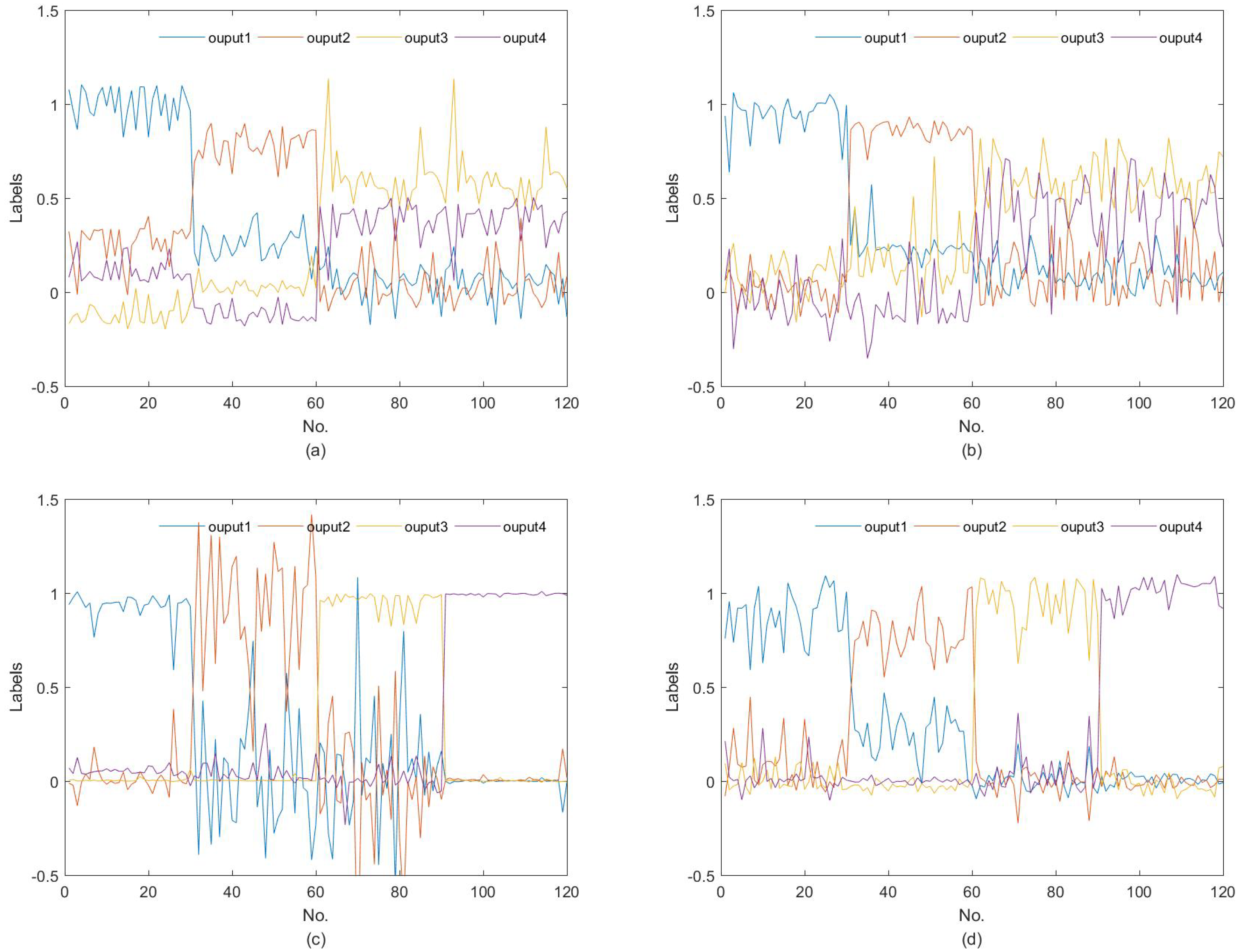
In this paper, 60 fusion features from each bearing state were constructed from the collected vibration signals. Thirty labeled samples were used to construct an SVM model, and the other 30 samples were employed for testing. From the description above, a fusion feature extraction strategy, including sensitive IMF selection and feature fusion of multiple sensors, was proposed to diagnose bearing faults with an SVM model. The BP neural network is a frequently used artificial intelligence classifier for fault diagnosis [32]. Therefore, we first implemented the BP neural network as the classifier to diagnose bearing faults to testify the availabilities of the proposed method. When constructing the results of the BP neural network model, its four goal outputs, marked output1, output2, output3, and output4, were coded with ‘0’ and ‘1’. In this paper, the goal outputs of states S1, S2, S3, and S4 are represented by ‘1000’, ‘0100’, ‘0010’, and ‘0001’, respectively.
Figure 11 displays the test results of the BP neural network. As can be observed from Figure 11a, output1, output2, output3, and output4 of these test samples with serial numbers 1–31 can be regarded as being close to ‘1’, ‘0’, ‘0’, and ‘0’, and they matched the goal outputs to some degree. However, the test results of the test samples with serial numbers 61–120 mismatched the goal outputs. In the same manner, the diagnosis results of Figure 11b–d can be analyzed. By contrastively analysing the plots in Figure 11, it can be observed that Figure 11d has the best classification effect, and the accuracy of Figure 11c is greater than that of Figure 11a,b. These experimental results demonstrate that the proposed sensitive IMF selection and fusion extraction method can improve the fault diagnosis accuracy.
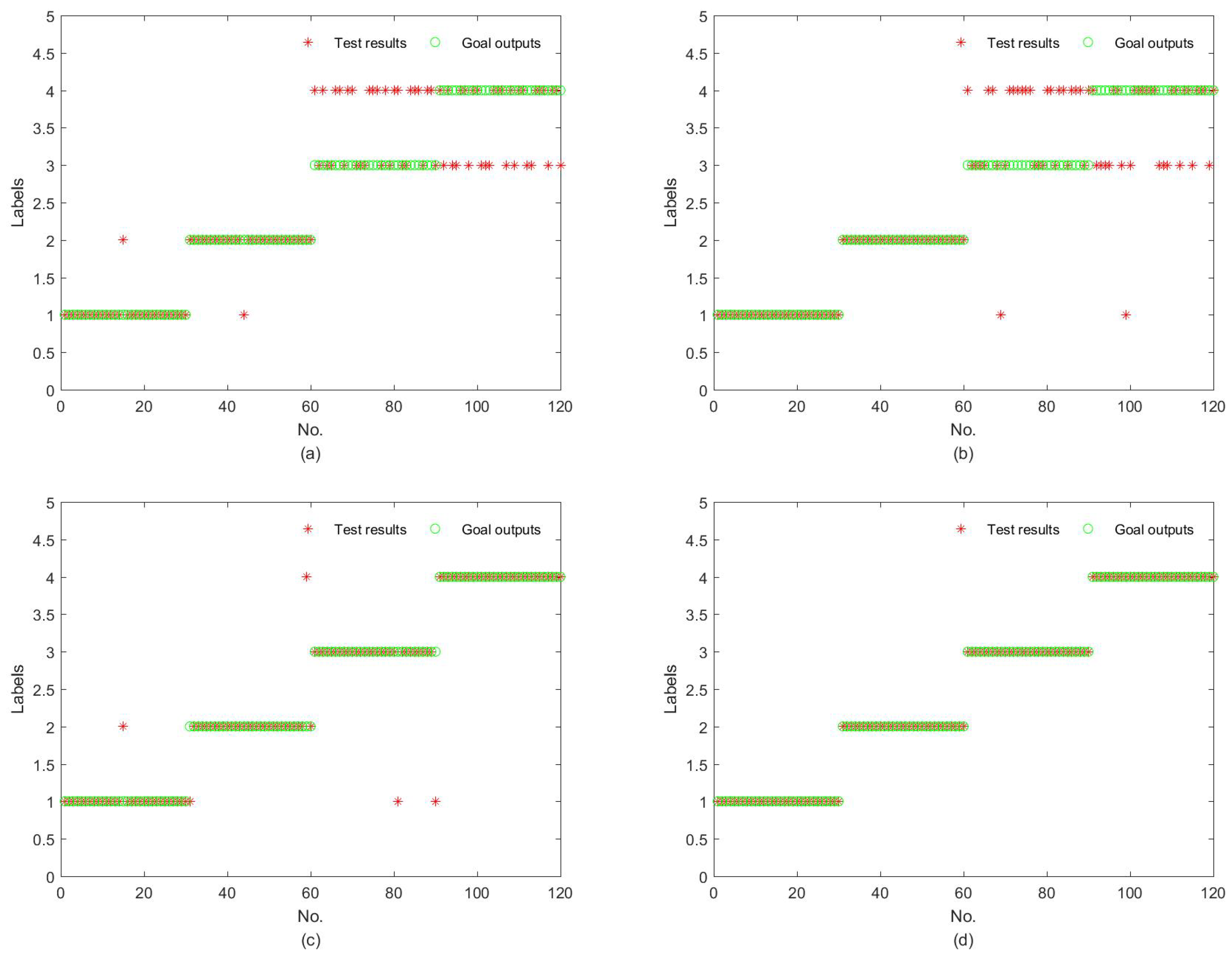
In this paper, SVM was used as the classifier for the bearing fault diagnosis. In the model construction stage, the target outputs of bearing states S1, S2, S3, and S4 were represented by digital coding ‘1’, ‘2’, ‘3’, and ‘4’, respectively. As 12 features can be extracted from each vibration signal of six sensors, features can be available to the classifier if all original features of the six sensors for the fault diagnosis are used. Figure 12 displays the fault diagnosis results of the SVM model; the test results and goal outputs are represented by different colors and shapes. By comparing the values of these test results and goal outputs in Figure 12a, it can be determined that the test results and goal outputs of some test samples did not coincide. That is, some test samples in Figure 12a were misdiagnosed. Similarly, the diagnosis accuracies of Figure 12b–d were analyzed and these are shown in Table 4. From this table, the diagnostic accuracy of three comparison methods and the proposed method are 73.33%, 74.17%, 95.83% and 100%, respectively. Moreover, the diagnosis accuracy of Figure 12c was also greater than that shown in Figure 12a and Figure 10b. To further analyze the robust performance of the proposed method, a 10-fold cross-validation is carried out with these used fusion features of Figure 10d, and the mean diagnostic accuracies of the proposed method is 98.75% which is acceptable for mechanical fault diagnosis. Therefore, we can conclude that the proposed method can effectively and accurately diagnose bearing faults.
5. Conclusions
To fully use the vibration signals of multi-sensors, a new information fusion approach was proposed for bearing fault diagnosis. This method employs ensemble empirical mode decomposition (EEMD) as the tool for vibration signal processing, correlation coefficient analysis as the method for sensitive IMFs selection and feature fusion, and support vector machine (SVM) as the classifier. Considering that the traditional signal processing method cannot deal with the nonlinear and non-stationary vibration signals generated by these bearings with various conditions, the EEMD algorithm was used to decompose these original signals into a set of intrinsic mode functions (IMFs). Not all components are helpful for fault diagnosis, and some will even interfere with fault diagnosis, so a correlation coefficient ratio factor (CCRF) is defined to select sensitive IMFs to reduce noise and reconstruct new vibration signals for further analysis. After that, an original feature space was constructed from the reconstructed signal, and the so-called fused features were extracted by original feature space and weights assigned by correlation coefficients among these vibration signals of considered multi-sensors. With this feature fusion algorithm, the dimension of final features was successfully reduced to one-sixth of the original feature space. Experiments were implemented to verify the performance of the proposed approach. The experimental results of the BP neural network showed that the proposed sensitive IMF selection and fusion extraction method can improve the fault diagnosis accuracy. The diagnosis results of original vibration signals, the first IMF, the proposed reconstruction signal, and the proposed method were 73.33%, 74.17%, 95.83% and 100%, respectively. Therefore, the experiments showed that the proposed method has the highest diagnostic accuracy, and it can be regarded as a new way to improve the diagnosis results for bearings.
Author Contributions
F.J. designed the experiments and analyzed the datasets; Z.Z., W.L. and Y.R. performed the experiments and analyzed part of the dataset; F.J., G.Z. and Y.C. wrote the paper. All authors contributed to discussing and revising the manuscript.
Funding
This work is supported by the National Natural Science Foundation of China (Nos. 51605478, U1510205, 51475455), the Natural Science Foundation of Jiangsu Province (No. BK20160251), the Fundamental Research Funds for the Central Universities (2017QNA17), and the project was funded by the Priority Academic Program Development of the Jiangsu Higher Education Institutions (PAPD).
Acknowledgments
The authors would like to thank all of the reviewers for their constructive comments.
Conflicts of Interest
The authors declare no conflict of interest.
References
- Yang, Y.; Wang, H.; Cheng, J.; Zhang, K. A fault diagnosis approach for roller bearing based on VPMCD under variable speed condition. Measurement 2013, 46, 2306–2312. [Google Scholar] [CrossRef]
- Wang, D.; Tse, P.W.; Tsui, K.L. An enhanced Kurtogram method for fault diagnosis of rolling element bearings. Mech. Syst. Signal Process. 2013, 35, 176–199. [Google Scholar] [CrossRef]
- Yang, Z.X.; Zhong, J.H. A hybrid EEMD-based sampEn and SVD for acoustic signal processing and fault diagnosis. Entropy 2016, 18, 112. [Google Scholar] [CrossRef]
- Randall, R. Vibration-Based Condition Monitoring; Wiley: New York, NY, USA, 2011. [Google Scholar]
- Li, Y.; Liang, X.; Zuo, M.J. Diagonal slice spectrum assisted optimal scale morphological filter for rolling element bearing fault diagnosis. Mech. Syst. Signal Process. 2017, 85, 146–161. [Google Scholar] [CrossRef]
- Zhang, S.; Lu, S.; He, Q.; Kong, F. Time-varying singular value decomposition for periodic transient identification in bearing fault diagnosis. J. Sound Vib. 2016, 379, 213–231. [Google Scholar] [CrossRef]
- Jardine, A.; Lin, D.; Banjevic, D. A review on machinery diagnostics and prognostics implementing condition-based maintenance. Mech. Syst. Signal Process. 2007, 20, 1483–1510. [Google Scholar] [CrossRef]
- Liu, Y.; Guo, L.; Wang, Q.; An, G.; Guo, M.; Lian, H. Application to induction motor faults diagnosis of the amplitude recovery method combined with FFT. Mech. Syst. Signal Process. 2010, 24, 2961–2971. [Google Scholar] [CrossRef]
- Miao, Q.; Cong, L.; Pecht, M. Identification of multiple characteristic components with high accuracy and resolution using the zoom interpolated discrete Fourier transform. Meas. Sci. Technol. 2011, 22, 55701. [Google Scholar] [CrossRef]
- Antoni, J.; Randall, R.B. The spectral kurtosis: Application to the vibratory surveillance and diagnostics of rotating machines. Mech. Syst. Signal Process. 2006, 20, 308–331. [Google Scholar] [CrossRef]
- Kankar, P.K.; Sharma, S.C.; Harsha, S.P. Rolling element bearing fault diagnosis using autocor relation and continuous wavelet transform. J. Vib. Control 2011, 17, 2081–2094. [Google Scholar] [CrossRef]
- Zhong, G.S.; Ao, L.P.; Zhao, K. Influence of explosion parameters on wavelet packet frequency band energy distribution of blast vibration. J. Cent. South Univ. 2012, 19, 2674–2680. [Google Scholar] [CrossRef]
- Jiang, F.; Zhu, Z.; Li, W.; Zhou, G.; Chen, G. Fault identification of rotor-bearing system based on ensemble empirical mode decomposition and self-zero space projection analysis. J. Sound Vib. 2014, 333, 3321–3331. [Google Scholar] [CrossRef]
- Huang, N.; Shen, Z.; Long, S.; Wu, M.; Shih, H.; Zheng, Q.; Yen, N.; Tung, C.; Liu, H. The empirical mode decomposition and the Hilbert spectrum for nonlinear and non-stationary time series analysis. Proc. R. Soc. Lond. Ser. A Math. Phys. Eng. Sci. 1998, 454, 903–995. [Google Scholar] [CrossRef]
- Du, Q.; Yang, S. Application of the EMD method in the vibration analysis of ball bearings. Mech. Syst. Signal Process. 2007, 21, 2634–2644. [Google Scholar] [CrossRef]
- Wu, F.; Qu, L. Diagnosis of subharmonic faults of large rotating machinery based on EMD. Mech. Syst. Signal Process. 2009, 23, 467–475. [Google Scholar] [CrossRef]
- Xiong, Q.; Xu, Y.; Peng, Y.; Zhang, W.; Li, Y.; Tang, L. Low-speed rolling bearing fault diagnosis based on EMD denoising and parameter estimate with alpha stable distribution. J. Mech. Sci. Technol. 2017, 31, 1587–1601. [Google Scholar] [CrossRef]
- Junsheng, C.; Dejie, Y.; Yu, Y. A fault diagnosis approach for roller bearings based on EMD method and AR model. Mech. Syst. Signal Process. 2006, 20, 350–362. [Google Scholar] [CrossRef]
- Ahn, J.H.; Kwak, D.H.; Koh, B.H. Fault detection of a roller-bearing system through the EMD of a wavelet denoised signal. Sensors 2014, 14, 15022–15038. [Google Scholar] [CrossRef] [PubMed]
- Wu, Z.; Huang, N.E. Ensemble empirical mode decomposition: A noise-assisted data analysis method. Adv. Adapt. Data Anal. 2009, 1, 1–41. [Google Scholar] [CrossRef]
- Yi, C.; Lin, J.; Zhang, W.; Ding, J. Faults diagnostics of railway axle bearings based on IMFs confidence index algorithm for ensemble EMD. Sensors 2015, 15, 10991–11011. [Google Scholar] [CrossRef] [PubMed]
- Zhao, H.; Sun, M.; Deng, W.; Yang, X. A New Feature Extraction Method Based on EEMD and Multi-Scale Fuzzy Entropy for Motor Bearing. Entropy 2017, 19, 14. [Google Scholar] [CrossRef]
- Chen, H.; Chen, P.; Chen, W.; Wu, C.; Li, J.; Wu, J. Wind Turbine Gearbox Fault Diagnosis Based on Improved EEMD and Hilbert Square Demodulation. Appl. Sci. 2017, 7, 128. [Google Scholar] [CrossRef]
- Wang, H.; Chen, J.; Dong, G. Feature extraction of rolling bearing’s early weak fault based on EEMD and tunable Q-factor wavelet transform. Mech. Syst. Signal Process. 2014, 48, 103–119. [Google Scholar] [CrossRef]
- Yang, H.; Ning, T.; Zhang, B.; Yin, X.; Gao, Z. An adaptive denoising fault feature extraction method based on ensemble empirical mode decomposition and the correlation coefficient. Adv. Mech. Eng. 2017, 9. [Google Scholar] [CrossRef] [Green Version]
- Li, H.; Li, M.; Li, C.; Li, F.; Meng, G. Multi-faults decoupling on turbo-expander using differential-based ensemble empirical mode decomposition. Mech. Syst. Signal Process. 2017, 93, 267–280. [Google Scholar] [CrossRef]
- Guo, W.; Tse, P.W. A novel signal compression method based on optimal ensemble empirical mode decomposition for bearing vibration signals. J. Sound Vib. 2013, 332, 423–441. [Google Scholar] [CrossRef]
- Lei, Y.; Zuo, M.J.; Hoseini, M. The use of ensemble empirical mode decomposition to improve bispectral analysis for fault detection in rotating machinery. Proc. Inst. Mech. Eng. Part C J. Mech. Eng. Sci. 2010, 224, 1759–1769. [Google Scholar] [CrossRef]
- Li, Z.; Yan, X.; Yuan, C.; Zhao, J.; Peng, Z. Fault detection and diagnosis of a gearbox in marine propulsion systems using bispectrum analysis and artificial neural networks. J. Mar. Sci. Appl. 2011, 10, 17–24. [Google Scholar] [CrossRef] [Green Version]
- Chen, J.; Hao, G. Research on the Fault Diagnosis of Wind Turbine Gearbox Based on Bayesian Networks. Pract. Appl. Intell. Syst. 2012, 124, 217–223. [Google Scholar]
- Raj, A.S.; Murali, N. Early classification of bearing faults using morphological operators and fuzzy inference. IEEE Trans. Ind. Electron. 2013, 60, 567–574. [Google Scholar] [CrossRef]
- Vyas, N.S.; Padhy, D.K. Fault identification in rotor-bearing systems through back-propagation and probabilistic neural networks. Proc. SPIE 2002, 4753, 271–277. [Google Scholar]
- Zhang, K.; Li, Y.; Scarf, P.; Ball, A. Feature selection for high-dimensional machinery fault diagnosis data using multiple models and Radial Basis Function networks. Neurocomputing 2011, 74, 2941–2952. [Google Scholar] [CrossRef]
- Samanta, B.; Al-Balushi, K.R.; Al-Araimi, S.A. Artificial neural networks and support vector machines with genetic algorithm for bearing fault detection. Eng. Appl. Artif. Intell. 2003, 16, 657–665. [Google Scholar] [CrossRef]
- Hu, Q.; He, Z.; Zhang, Z.; Zi, Y. Fault diagnosis of rotating machinery based on improved wavelet package transform and SVMs ensemble. Mech. Syst. Signal Process. 2007, 21, 688–705. [Google Scholar] [CrossRef]
- Ni, J.; Zhang, C.; Ren, L.; Yang, S.X. Abrupt event monitoring for water environment system based on KPCA and SVM. IEEE Trans. Instrum. Meas. 2012, 61, 980–989. [Google Scholar] [CrossRef]
- Bordoloi, D.J.; Tiwari, R. Optimum multi-fault classification of gears with integration of evolutionary and SVM algorithms. Mech. Mach. Theory 2014, 73, 49–60. [Google Scholar] [CrossRef]
- Vapnik, V.N. The Nature of Statistical Learning Theory; Springer: New York, NY, USA, 1999. [Google Scholar]
- Jafarian, P.; Sanaye-Pasand, M. High-frequency transients-based protection of multiterminal transmission lines using the SVM technique. IEEE Trans. Power Deliv. 2013, 28, 188–196. [Google Scholar] [CrossRef]
- Lei, Y.; He, Z.; Zi, Y. EEMD method and WNN for fault diagnosis of locomotive roller bearings. Expert Syst. Appl. 2011, 38, 7334–7341. [Google Scholar] [CrossRef]
- Peng, Z.K.; Tse, P.W.; Chu, F.L. An improved Hilbert-Huang transform and its application in vibration signal analysis. J. Sound Vib. 2005, 286, 187–205. [Google Scholar] [CrossRef]
- Li, Z.; Yan, X.; Yuan, C.; Peng, Z.; Li, L. Virtual prototype and experimental research on gear multi-fault diagnosis using wavelet-autoregressive model and principal component analysis method. Mech. Syst. Signal Process. 2011, 25, 2589–2607. [Google Scholar] [CrossRef]
- Cao, J.; Chen, L.; Zhang, J.; Cao, W. Fault diagnosis of complex system based on nonlinear frequency spectrum fusion. Measurement 2012, 46, 125–131. [Google Scholar] [CrossRef]
- Khaleghi, B.; Khamis, A.; Karray, F.O.; Razavi, S.N. Multisensor data fusion: A review of the state-of-the-art. Inf. Fusion 2013, 14, 28–44. [Google Scholar] [CrossRef]
- Rubini, R.; Meneghetti, U. Application of the envelope and wavelet transform analysis for the diagnosis of incipient faults in ball bearings. Mech. Syst. Signal Process. 2001, 15, 287–302. [Google Scholar] [CrossRef]
- Jiang, F.; Zhu, Z.; Li, W.; Chen, G.; Zhou, G. Robust condition monitoring and fault diagnosis of rolling element bearings using improved EEMD and statistical features. Meas. Sci. Technol. 2014, 25, 25003. [Google Scholar] [CrossRef]
Figure 1.
Main procedure of the presented method.

Figure 2.
Multi-function mechanical fault simulator: (1) AC motor, (2) sensor, (3) shaft, (4) rotor disc, (5) test bearing, (6) outboard bearing housing, (7) normal bearing, (8) inboard bearing housing, (9) flexible coupling, (10) converter.
Figure 2.
Multi-function mechanical fault simulator: (1) AC motor, (2) sensor, (3) shaft, (4) rotor disc, (5) test bearing, (6) outboard bearing housing, (7) normal bearing, (8) inboard bearing housing, (9) flexible coupling, (10) converter.

Figure 3.
Bearings with different faulty conditions.

Figure 4.
Sensor installation diagram.

Figure 5.
Waves of vibration signals under normal condition.

Figure 6.
Waves of vibration signals under inner-race fault.

Figure 7.
Waves of vibration signals under ball fault.

Figure 8.
Waves of vibration signals under outer-race fault.

Figure 9.
Waves of vibration signals in time and frequency domain under four bearing conditions.

Figure 10.
Vibration signals collected from Sensor 6 and the decomposition results of EEMD: (a) normal IMFs; (b) IMFs of inner-race fault; (c) IMFs of ball fault; (d) IMFs of outer-race fault.
Figure 10.
Vibration signals collected from Sensor 6 and the decomposition results of EEMD: (a) normal IMFs; (b) IMFs of inner-race fault; (c) IMFs of ball fault; (d) IMFs of outer-race fault.

Figure 11.
Test results of the BP neural network where the features used were extracted from (a) the vibration signals of six sensors; (b) the first IMF of six sensors; (c) reconstructed vibration signals using the proposed sensitive IMF collection method; (d) reconstructed vibration signals using the proposed feature fusion method.

Figure 12.
Test results of the support vector machine (SVM) model where the features used were extracted from (a) the vibration signals of six sensors; (b) the first IMF of six sensors; (c) reconstructed vibration signals using the proposed sensitive IMFs collection method; (d) reconstructed vibration signals using the proposed feature fusion method.


Table 1.
Some key technical characteristics of used bearings.
| Items | Type | Number of Rolling Elements | Pitch Diameter | Rolling Elements Diameter |
|---|---|---|---|---|
| Components | ER-12k | 8 | 1.318 inches | 0.3125 inches |
Table 2.
CCRF values of IMFs decomposed from vibration signals collected by Sensor 6.
| Conditions | IMF1 | IMF2 | IMF3 | IMF4 | IMF5 | IMF6 | IMF7 | IMF8 | IMF9 | IMF10 |
|---|---|---|---|---|---|---|---|---|---|---|
| S1 | 0.6672 | 0.6817 | 0.5388 | 0.1293 | 0.0328 | 0.0520 | 0.0124 | 0.0091 | 0.0093 | 0.0036 |
| S2 | 62.6646 | 28.4247 | 1.4968 | 1.2401 | 1.0390 | 0.1951 | 0.0190 | 0.0138 | 0.0102 | 0.0191 |
| S3 | 251.5411 | 2.1859 | 1.5832 | 0.4112 | 0.9304 | 0.0021 | 0.0194 | 3.3 | 1.1 | 5.3 |
| S4 | 55.0147 | 50.8732 | 9.4266 | 0.7410 | 0.1520 | 0.0435 | 0.0083 | 0.0110 | 0.0043 | 0.0114 |
Table 3.
Group weight values of six sensors under four conditions.
| Conditions | Sensor 1 | Sensor 2 | Sensor 3 | Sensor 4 | Sensor 5 | Sensor 6 |
|---|---|---|---|---|---|---|
| S1 | 0.4214 | 0.0244 | 0.4368 | 0.0585 | 0.0184 | 0.0406 |
| S2 | 0.3958 | 0.0312 | 0.4183 | 0.0617 | 0.0580 | 0.0350 |
| S3 | 0.3897 | 0.0898 | 0.3949 | 0.0450 | 0.0446 | 0.0360 |
| S4 | 0.3548 | 0.0060 | 0.3434 | 0.1068 | 0.0789 | 0.1102 |
Table 4.
Comparison of the proposed method with commonly applied classifiers.
| Experiments | Features per Sample | Test Samples | Accuracy(%) |
|---|---|---|---|
| SVM + features of vibration signal | 30 | 73.33 | |
| SVM + features of first IMF | 30 | 74.17 | |
| SVM + features of reconstruction signal | 30 | 95.83 | |
| Proposed method | 30 | 100 |
© 2018 by the authors. Licensee MDPI, Basel, Switzerland. This article is an open access article distributed under the terms and conditions of the Creative Commons Attribution (CC BY) license (http://creativecommons.org/licenses/by/4.0/).
Share and Cite
MDPI and ACS Style
Jiang, F.; Zhu, Z.; Li, W.; Ren, Y.; Zhou, G.; Chang, Y. A Fusion Feature Extraction Method Using EEMD and Correlation Coefficient Analysis for Bearing Fault Diagnosis. Appl. Sci. 2018, 8, 1621. https://doi.org/10.3390/app8091621
AMA Style
Jiang F, Zhu Z, Li W, Ren Y, Zhou G, Chang Y. A Fusion Feature Extraction Method Using EEMD and Correlation Coefficient Analysis for Bearing Fault Diagnosis. Applied Sciences. 2018; 8(9):1621. https://doi.org/10.3390/app8091621
Chicago/Turabian StyleJiang, Fan, Zhencai Zhu, Wei Li, Yong Ren, Gongbo Zhou, and Yonggen Chang. 2018. "A Fusion Feature Extraction Method Using EEMD and Correlation Coefficient Analysis for Bearing Fault Diagnosis" Applied Sciences 8, no. 9: 1621. https://doi.org/10.3390/app8091621
Note that from the first issue of 2016, this journal uses article numbers instead of page numbers. See further details here.