Double Low-Rank and Sparse Decomposition for Surface Defect Segmentation of Steel Sheet

Featured Application

The proposed DLRSD-based segmentation method can be applied for other industrial products, such as glass, fabric, LCD and AMOLED.

Abstract

Surface defect segmentation supports real-time surface defect detection system of steel sheet by reducing redundant information and highlighting the critical defect regions for high-level image understanding. Existing defect segmentation methods usually lack adaptiveness to different shape, size and scale of the defect object. Based on the observation that the defective area can be regarded as the salient part of image, a saliency detection model using double low-rank and sparse decomposition (DLRSD) is proposed for surface defect segmentation. The proposed method adopts a low-rank assumption which characterizes the defective sub-regions and defect-free background sub-regions respectively. In addition, DLRSD model uses sparse constrains for background sub-regions so as to improve the robustness to noise and uneven illumination simultaneously. Then the Laplacian regularization among spatially adjacent sub-regions is incorporated into the DLRSD model in order to uniformly highlight the defect object. Our proposed DLRSD-based segmentation method consists of three steps: firstly, using DLRSD model to obtain the defect foreground image; then, enhancing the foreground image to establish the good foundation for segmentation; finally, the Otsu’s method is used to choose an optimal threshold automatically for segmentation. Experimental results demonstrate that the proposed method outperforms state-of-the-art approaches in terms of both subjective and objective tests. Meanwhile, the proposed method is applicable to industrial detection with limited computational resources.

1. Introduction

Surface defect detection plays an important role in quality enhancement in industrial product manufacturing. However, traditional defect detection is performed by human eyes, which yields low efficiency and high missing rate. Currently, vision-based automated defect detection has drawn much attention, which has important theoretical and practical value [1,2,3,4]. In automatic surface inspection of steel sheet, segmentation of surface defect is a significant step, which generates a binary map to identify defects. In the past two decades, commonly-used segmentation methods can be classified into three categories: statistical-based methods, filter-based methods and model-based methods. Statistical-based methods, such as Otsu’s method [5], gray level co-occurrence matrix, local binary pattern, maximum entropy, region growing and morphological watersheds, are used to evaluate the spatial distribution of pixel intensities for segmentation. Filter-based methods, such as discrete Fourier transform [6], discrete Gabor transform [7] and discrete wavelet transform [8,9], apply a bank of filters to the image, in which the energies of the filters response are utilized as features to segment the defects. Model-based approaches obtain certain models with specific feature distributions or other attributes using diverse descriptors, for instance, level set, fuzzy theory, partial differential equations and texture patterns.

Most recently, with the development of saliency detection technology, segmentation methods that use saliency map are gradually rising in the industrial defect inspection field. This method constructs a saliency map that highlights the defect regions standing out from the rest of the image, which provide the good foundation for segmentation. Guan et al. [10] proposed saliency map construction method using Gaussian pyramid decomposition. Then segmentation is conducted with the saliency map. This model exhibits good performance for strip steel defect detection. Li et al. [11] devised a low-rank representation-based saliency detection model for textile fabric defect detection. Zhao et al. [12] also presented a novel saliency detection model, which obviously improve the accuracy of automated defect segmentation.

These methods achieve good results on defect segmentation for a certain and homogeneous texture, but remain a challenging issue for segmentation with miscellaneous textures due to random disturbance. Specially, as the surface defect image of steel sheet has a low signal-to-noise ratio, low contrast between defect object and background, heterogeneous and scattered defect, cluttered and complicated background, these methods still lack of accuracy and suffer from limited adaptability and robustness in industrial practice.

Usually, a defect-free surface in industrial products has consistent texture. The emergence of defects can be regarded as the foreground object superposed in the regular-texture background. As shown in Figure 1, a surface defect image of steel sheet $I$ is decomposed into two parts: relatively homogeneous background image $B$ and a defect foreground image $F$ that is the desired image for the following segmentation.

Inspired by the above analysis, an easy-to-implement method based on double low-rank and sparse decomposition (DLRSD) is proposed in this paper for surface defect segmentation. Considering double low-rank and sparse characteristics of surface defect image, combined with a local consistency constrain among spatially adjacent sub-regions by imposing Laplacian regularization, the feature matrix that form by $I$ can be adaptively decomposed into foreground feature matrix that form by defect foreground image $F$ and background feature matrix that form by background image $B$ in a certain feature space, respectively. Specifically, the foreground image $F$ is served as the source image for segmentation, which can better cope with the intra-class variations and background clutters, leading to a higher performance. Theoretical analysis and experimental results demonstrate the feasibility and effectiveness of the proposed DLRSD-based segmentation method for the surface defect of steel sheet. At the same time, it provides an interesting perspective for the industrial product’s surface defect segmentation.

The rest of this paper is organized as follows. In Section 2, we review some existing saliency detection methods, especially the structural matrix decomposition-based methods. In Section 3 we introduce the proposed DLRSD model, including formulation and optimization. Section 4 presents the DLRSD-based defect segmentation method. Also, we give more detail on enhancing the original defect foreground image. Section 5 describes experimental results between our proposed method and some state-of-the-art methods. Finally, conclusions are given in Section 6.

2. Related Work

During the past few years, there are many methods attempting to segment the salient object from the saliency map of an input image [13,14,15,16,17,18,19]. The quality and effectiveness of segmentation are decided by the quality of saliency map [20]. Based on the milestone work, some structural matrix decomposition-based methods transform a saliency detection problem into a feature subspace decomposition problem, which can improve detection results in terms of both speed and accuracy. Particularly, many studies conclude that low-rank matrix decomposition-based methods can obtain better saliency detection performance. These methods assume that an image can be represented as a combination of a highly redundant part (e.g., visually consistent background regions) and a sparse part (e.g., salient object foreground regions). Therefore, given the feature matrix of an input image, it can be decomposed into a low-rank matrix corresponding to the non-salient background and a sparse matrix corresponding to the salient foreground objects. Yan et al. [21] employed sparse coding as a feature representation vector of image. Zou et al. [22] designed multi-scale superpixel segmentation to construct the feature matrix and prior matrix. Although Shen et al. [23] adopted learnt linear transformation of the feature space to integrate low-level features and high-level prior knowledge, the learnt transform matrix is correlated for training data set. Unfortunately, the sparsity assumption of the salient objects can’t be guaranteed universally, especially when the salient objects with big size occupy most of the image, and then suffer from limited adaptability. Therefore, Peng et al. [24] developed tree-structured sparsity-inducing regularization and Laplacian regularization to disentangle the salient objects and background precisely, and then obtained competitive results. But it may be difficult to suppress some small background regions with distinctive appearances because of the constructed index-tree is not precise enough. Subsequently, Sun et al. [25] presented diversity-induced regularization based on Hilbert–Schmidt independence criterion, which make the background much cleaner in the saliency map and boost the saliency detection performance. But, they don’t consider the low-rank characteristic for the foreground regions and background regions simultaneously, and ignore the spatial and pattern relations of image regions, which may lead to very noisy saliency map and influences on the final segmentation performance.

To solve the problems mentioned above, the proposed DLRSD model considers the correlation between defective regions and defect-free regions, which is different from existing methods in essence. Besides, it uses the nuclear norm to depict the low-rank property of defect object rather than consider it as the sparse noises, which can produce more accurate and reliable saliency map that represents the defect foreground image.

3. Double Low-Rank and Sparse Decomposition Model

In this section, we will introduce the proposed DLRSD model and optimization procedure in details.

3.1. Problem Formulation

Let $\left\{R_1, R_2, \cdots , R_K\right\}$ be a set of $K$ non-overlapping sub-regions of a surface defect image $I$, all the feature vectors of sub-regions can construct the feature matrix $D$. The proposed DLRSD model is to design an effective model to decompose the feature matrix $D$ into a feature matrix $S$ that represents a defect foreground image $F$ and a feature matrix $L$ that represents a background image $B$:

$$D=S+L$$

(1)

In order to separate defect regions and background regions accurately, some constrains are needed for characterizing two feature matrices $S$ and $L$. According to the surface defect image $I$ that is pre-processed by superpixel segmentation, both defect foreground and background contain multiple homogeneous and highly similar sub-regions, for each defective sub-region, the corresponding locations in saliency map has high probability in larger brightness, indicating that it has higher saliency value. Besides, different defective sub-regions are highly correlated and the corresponding feature vectors lie in a low-dimensional subspace. Therefore, the feature matrix $S$ is expected to be low-rank. Meanwhile, most of background sub-regions tend to have lower saliency value. They are strongly correlated and lie in a low-dimensional feature subspace that is independent of the defect foreground subspace. The strong correlations among the background sub-regions suggest that feature matrix $L$ may have the low-rank property. What is more, in order to reduce the influence of noises and enhance the robustness to uneven illumination, we assume that the background lies in a sparse feature subspace and can be characterized by a sparse matrix.

Based on above analysis, the structured matrix decomposition model can be constructed as follows:

$$\begin{array}{l}\underset{L,S}{\min }\left(\mathrm{rank}\left(L\right)+\alpha \mathrm{rank}\left(S\right)+\beta \Theta \left(S,L\right)+\gamma {\left|\right|L\left|\right|}_0\right)\hfill \\ \mathrm{s}.\mathrm{t}.D=S+L\hfill \end{array}$$

(2)

where $\mathrm{rank}(·)$ denotes the rank of matrix; ${\left|\right|·\left|\right|}_0$ denotes $l_0$ norm of matrix, which equals the number of non-zero element of matrix; $\Theta \left(S,L\right)$ denotes the regularization to enlarge the margin and reduce the coherence between the feature subspaces induced by $S$ and $L$; $D\in {ℝ}^{d\times K}$ represents the feature matrix; $\alpha >0$, $\beta >0$ and $\gamma >0$ are regularization parameters.

To separate the defect object from the background easily, spatially adjacent sub-regions with smaller spatial distance and more similar feature vector should be assigned to similar and higher weight values, the local invariance assumption [26] based Laplacian regularization $\Theta \left(S,L\right)$ [24] can be defined as follows:

$$\Theta \left(S,L\right)=\frac{1}{2}{\displaystyle \sum }_{i,j=1}^K||{\mathit{s}}_i-{\mathit{s}}_j{\left|\right|}_2^2{w}_{ij}=\mathrm{tr}\left(SM{S}^T\right)$$

(3)

where $\mathrm{tr}(·)$ denotes the trace of a matrix; $s_i$ denotes the i-th column of matrix $S$; the element $w_{ij}$ of affinity matrix $W\in {ℝ}^{K\times K}$ denotes the weight that represents the feature similarity between sub-regions $R_i$ and $R_j$; $M\in {ℝ}^{K\times K}$ is a Laplacian matrix.

According to the undirected graph model from a surface defect image, each sub-region is represented by a node, the affinity matrix $W$ is

$$w_{ij}=\{\begin{array}{ll}\exp \left(\frac{-\left|\right|{\mathit{p}}_i-{\mathit{p}}_j{\left|\right|}_2^2}{2{\sigma }_{\mathit{p}}^2}\right)\exp \left(\frac{-\left|\right|{\overline{\mathit{f}}}_i-{\overline{\mathit{f}}}_j{\left|\right|}_2^2}{2{\sigma }_{\mathit{f}}^2}\right)& R_i \mathrm{and} R_j \mathrm{are} \mathrm{spatially} \mathrm{adjacent} \\ 0& \mathrm{otherwise}\end{array}$$

(4)

where ${\mathit{p}}_i\in {ℝ}^2$ and ${\mathit{p}}_j\in {ℝ}^2$ denote the central coordinate of $R_i$ and $R_j$; ${\overline{\mathit{f}}}_i\in {ℝ}^d$ and ${\overline{\mathit{f}}}_j\in {ℝ}^d$ denote the feature vector of $R_i$ and $R_j$; $\exp \left(\frac{-\left|\right|{\mathit{p}}_i-{\mathit{p}}_j{\left|\right|}_2^2}{2{\sigma }_{\mathit{p}}^2}\right)$ represents spatial connectivity between $R_i$ and $R_j$, which represents the spatial contiguity; $\exp \left(\frac{-\left|\right|{\overline{\mathit{f}}}_i-{\overline{\mathit{f}}}_j{\left|\right|}_2^2}{2{\sigma }_{\mathit{f}}^2}\right)$ gives the feature similarity between $R_i$ and $R_j$; ${\sigma }_{\mathit{p}}$ and ${\sigma }_{\mathit{f}}$ are two scalars.

The Laplacian matrix $M$ is

$$M_{ij}=\{\begin{array}{l}-w_{ij} \hspace{1em}i\ne j \hfill \\ {\displaystyle \sum _{i\ne j}}{w}_{ij} \mathrm{otherwise}\hfill \end{array}$$

(5)

In particular, the Laplacian regularization $\Theta \left(S,L\right)$ can preserve the local consistency and invariance among the spatially adjacent sub-regions with similar saliency values in saliency maps. More specifically, the defect foreground is more uniformly highlighted and the background noise is also better suppressed, and eventually separates the defect from the background as much as possible.

3.2. Optimization

As $\mathrm{rank}(·)$ and ${\left|\right|·\left|\right|}_0$ are not convex, Equation (2) is NP-hard problem. A common heuristic criterion is to replace $\mathrm{rank}(·)$ and ${\left|\right|·\left|\right|}_0$ are replaced by nuclear norm ${\left|\right|·\left|\right|}_{*}$ and $l_1$ norm ${\left|\right|·\left|\right|}_1$ respectively. It has been shown that nuclear norm-based models can obtain the optimal low-rank solution in many kinds of applications [27,28]. Then, Equation (2) can be converted to the following convex surrogate optimization problem:

$$\begin{array}{l}\underset{L,S}{\min }\left({\left|\right|L\left|\right|}_{*}+\alpha {\left|\right|S\left|\right|}_{*}+\beta \mathrm{tr}\left(SM{S}^T\right)+\gamma {\left|\right|L\left|\right|}_1\right)\hfill \\ \mathrm{s}.\mathrm{t}.D=S+L\hfill \end{array}$$

(6)

where ${\left|\right|·\left|\right|}_{*}$ equals the sum of singular values of matrix; ${\left|\right|·\left|\right|}_1$ equals the sum of the absolute values of each element of matrix. For a matrix $A=a_{ij}\in {ℝ}^{m\times n}$, ${\left|\right|A\left|\right|}_{\mathit{p}}={\left({\displaystyle \sum }_{i=1}^m{\displaystyle \sum }_{j=1}^n{\left|a_{ij}\right|}^{\mathit{p}}\right)}^{\frac{1}{\mathit{p}}}$.

To solve Equation (6) efficiently, the alternating direction method (ADM) algorithm [29] can be adopted. By introducing the auxiliary variables $H$ and $J$, the augmented Lagrange function is given as follows:

$$\begin{array}{l}O\left(L,S,H,J,Y_1,Y_2,Y_3,\mu \right)\hfill \\ ={\left|\right|L\left|\right|}_{*}+\alpha {\left|\right|S\left|\right|}_{*}+\beta \mathrm{tr}\left(HM{H}^T\right)+\gamma {\left|\right|J\left|\right|}_1\hfill \\ \hspace{1em}+\mathrm{tr}\left(Y_1^T\left(D-L-S\right)\right)+\frac{\mu }{2}\left|\right|D-L-{S\left|\right|}_F^2\hfill \\ \hspace{1em}+\mathrm{tr}\left(Y_2^T\left(H-S\right)\right)+\frac{\mu }{2}\left|\right|H-{S\left|\right|}_F^2\hfill \\ \hspace{1em}+\mathrm{tr}\left(Y_3^T\left(J-L\right)\right)+\frac{\mu }{2}\left|\right|J-{L\left|\right|}_F^2\hfill \end{array}$$

(7)

where ${\left|\right|·\left|\right|}_F^2$ denotes the Frobenius norm of matrix, which is defined as the sum of squares of each element of matrix; $Y_1$, $Y_2$ and $Y_3$ are Lagrange multipliers; $\mu >0$ is a penalty parameter.

Therefore, Equation (7) can be converted to the following equivalent optimization problem:

$$\begin{array}{l}O\left(L,S,H,J,Y_1,Y_2,Y_3,\mu \right)\hfill \\ =\frac{1}{2}\left|\right|D-L-S+{\frac{Y_1}{\mu }\left|\right|}_F^2+\frac{1}{2}\left|\right|H-S+{\frac{Y_2}{\mu }\left|\right|}_F^2+\frac{1}{2}\left|\right|J-L+{\frac{Y_3}{\mu }\left|\right|}_F^2\hfill \\ \hspace{1em}+\frac{1}{\mu }{\left|\right|L\left|\right|}_{*}+\frac{\alpha }{\mu }{\left|\right|S\left|\right|}_{*}+\frac{\beta }{\mu }\mathrm{tr}\left(HM{H}^T\right)+\frac{\gamma }{\mu }{\left|\right|J\left|\right|}_1\hfill \end{array}$$

(8)

The above optimization problem can be solved by alternately updating one variable while others fixed. The detailed ADM algorithm for proposed DLRSD model is summarized in Algorithm 1.

(1) Updating $H$

In order to solve $H$, the optimal solution can be obtained by Equation (9):

$$\underset{H}{\min }\left(\frac{1}{2}\left|\right|H-S+{\frac{Y_2}{\mu }\left|\right|}_F^2+\frac{\beta }{\mu }\mathrm{tr}\left(HM{H}^T\right)\right)$$

(9)

Differentiating it with respect to $H$, and let it to be zero, therefore

$$H-S+\frac{Y_2}{\mu }+\frac{2\beta }{\mu }HM=0$$

(10)

The close-form solution can be obtained as follows:

$$H^{*}=\left(S-\frac{Y_2}{\mu }\right){\left(I+\frac{2\beta }{\mu }M\right)}^{-1}$$

(11)

(2) Updating $J$

In order to solve $J$, the optimal solution can be obtained by Equation (12):

$$\underset{J}{\min }\left(\frac{1}{2}{\left|\right|L-\frac{Y_3}{\mu }-J\left|\right|}_F^2+\frac{\gamma }{\mu }{\left|\right|J\left|\right|}_1\right)$$

(12)

The solution is

$$J^{*}={\Psi }_{\frac{\gamma }{\mu }}\left(L-\frac{Y_3}{\mu }\right)$$

(13)

where ${\Psi }_{\frac{\gamma }{\mu }}(·)$ denotes soft-thresholding shrinkage operator, which is defined as

$${\Psi }_{\frac{\gamma }{\mu }}\left(T\right)=\mathrm{sgn}\left(T\right)\max \left(\left|T\right|-\frac{\gamma }{\mu },0\right)=\{\begin{array}{ll}{T}_{ij}-\frac{\gamma }{\mu }\hfill & \hspace{1em}{T}_{ij}>\frac{\gamma }{\mu }\hfill \\ 0\hfill & \hspace{1em}-\frac{\gamma }{\mu }\le T_{ij}\le \frac{\gamma }{\mu }\hfill \\ T_{ij}+\frac{\gamma }{\mu }\hfill & \hspace{1em}{T}_{ij}<-\frac{\gamma }{\mu }\hfill \end{array}$$

(14)

where $T$ denotes a matrix, $T_{ij}$ denotes the $\left(i,j\right)$-th element of $T$, $\mathrm{sgn}\left(T\right)$ is the matrix whose entries are the signs of those of $T$.

(3) Updating $L$

In order to solve $L$, the optimal solution can be obtained by Equation (15):

$$\begin{array}{c}\underset{L}{\min }\left(\frac{1}{2}{\left|\right|D-S+\frac{Y_1}{\mu }-L\left|\right|}_F^2+\frac{1}{2}{\left|\right|J+\frac{Y_3}{\mu }-L\left|\right|}_F^2+\frac{1}{\mu }{\left|\right|L\left|\right|}_{*}\right)\end{array}$$

(15)

It can be rewritten as follows:

$$\underset{L}{\min }\left(\frac{1}{2}{\left|\right|\frac{1}{2}\left(D-S+J+\frac{Y_1+Y_3}{\mu }\right)-L\left|\right|}_F^2+\frac{1}{4\mu }{\left|\right|L\left|\right|}_{*}\right)$$

(16)

Its solution is

$$L^{*}=U{\Psi }_{\frac{1}{4\mu }}\left(\Sigma \right)V^T$$

(17)

where $\left(U,\Sigma ,V\right)=\mathrm{svd}\left[\frac{1}{2}\left(D-S+J+\frac{Y_1+Y_3}{\mu }\right)\right]$, $\mathrm{svd}(·)$ denotes singular value decomposition operator.

(4) Updating $S$

In order to solve $S$, the optimal solution can be obtained by Equation (18):

$$\begin{array}{c}\underset{S}{\min }\left(\frac{1}{2}{\left|\right|D-L+\frac{Y_1}{\mu }-S\left|\right|}_F^2+\frac{1}{2}\left|\right|H+\frac{Y_2}{\mu }-{S\left|\right|}_F^2+\frac{\alpha }{\mu }{\left|\right|S\left|\right|}_{*}\right)\end{array}$$

(18)

It can be rewritten as follows:

$$\underset{S}{\min }\left(\frac{1}{2}{\left|\right|\frac{1}{2}\left(D-L+H+\frac{Y_1+Y_2}{\mu }\right)-S\left|\right|}_F^2+\frac{\alpha }{4\mu }{\left|\right|S\left|\right|}_{*}\right)$$

(19)

Its solution is

$$S^{*}=U{\Psi }_{\frac{\alpha }{4\mu }}\left(\Sigma \right)V^T$$

(20)

where $\left(U,\Sigma ,V\right)=\mathrm{svd}\left[\frac{1}{2}\left(D-L+H+\frac{Y_1+Y_2}{\mu }\right)\right]$.

(5) Updating $Y_1$, $Y_2$ and $Y_3$

$$\begin{array}{l}{Y}_1=Y_1+\mu \left(D-L-S\right)\hfill \\ Y_2=Y_2+\mu \left(H-S\right)\hfill \\ Y_3=Y_3+\mu \left(J-L\right)\hfill \end{array}$$

(21)

(6) Updating $\mu$

$$\mu =\min \left(\rho \mu ,{\mu }_{\max }\right)$$

(22)

where $0<\rho <1$.

Algorithm 1 Solving DLRSD via ADM

Input: Data matrix $D\in {ℝ}^{d\times K}$, parameters $\alpha >0$, $\beta >0$, $\gamma >0$ and $ϵ>0$

Output: The optimal solution $L^{*}\in {ℝ}^{d\times K}$ and $S^{*}\in {ℝ}^{d\times K}$

1: Initializing

$L=S=H=J=0$, $Y_1=Y_2=Y_3=0$$\mu ={10}^{-1}$, ${\mu }_{max}={10}^{10}$, $\rho =1.1$, $NUM=100$, $k=1$

While $k\le NUM$ OR ${\left|\right|D-L-S\left|\right|}_F^2<ϵ$, ${\left|\right|H-S\left|\right|}_F^2<ϵ$, ${\left|\right|J-L\left|\right|}_F^2<ϵ$

2: Updating $H$

$H^{*}=\left(S-\frac{Y_2}{\mu }\right){\left(I+\frac{2\beta }{\mu }M\right)}^{-1}$

3: Updating $J$

$J^{*}={\Psi }_{\frac{\gamma }{\mu }}\left(L-\frac{Y_3}{\mu }\right)$

4: Updating $L$

$L^{*}=U{\Psi }_{\frac{1}{4\mu }}\left(\Sigma \right)V^T$

5: Updating $S$

$S^{*}=U{\Psi }_{\frac{\alpha }{4\mu }}\left(\Sigma \right)V^T$

6: Updating $Y_1$, $Y_2$ and $Y_3$

$\begin{array}{l}{Y}_1=Y_1+\mu \left(D-L-S\right)\hfill \\ Y_2=Y_2+\mu \left(H-S\right)\hfill \\ Y_3=Y_3+\mu \left(J-L\right)\hfill \end{array}$

7: Updating $\mu$

$\mu =\min \left(\rho \mu , {\mu }_{\max }\right)$

8: Iteration   $k=k+1$

End While

4. DLRSD-Based Surface Defect Segmentation

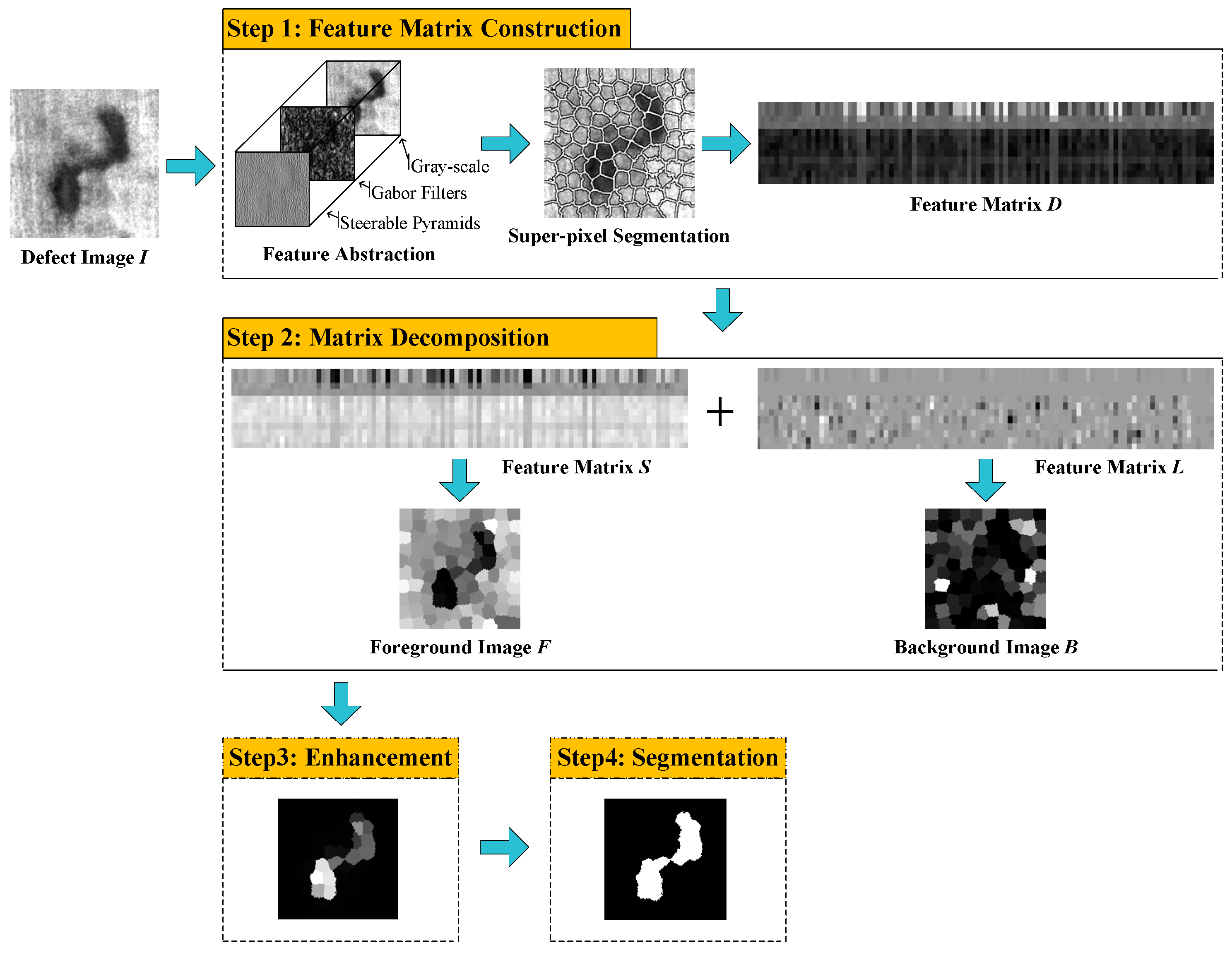
In this section, we describe how to apply the proposed DLRSD model to surface defect segmentation. The segmentation method has three stages. In first stage, we use DLRSD model to obtain the defect foreground image $F$. While in second stage, we utilize regression optimization to enhance $F$. At last, the segmentation is finished by Otsu’s method. The framework of DLRSD-based segmentation method is shown in Figure 2, the detailed procedure is summarized in Algorithm 2.

4.1. Feature Matrix Construction

According to [23,24], for each pixel ${\left\{I_i\right\}}_{i=1,2,\dots ,N}$ of a surface defect image $I$, where $N$ denotes the number of pixels, different types of low-level visual features, including gray-scale, Gabor filters and steerable pyramids, are extracted.

(1) Gray-scale

The pixel value of each pixel in defect image $I$ is extracted for gray-scale feature, which is normalized by subtracting its mean value over the entire image.

(2) Gabor filters

Gabor filters responses with eight directions on two different scales are performed on the defect image $I$, yielding 16 filter responses for each pixel.

(3) Steerable pyramids

Steerable pyramid filters with four directions on two different scales are performed on the defect image $I$, yielding 8 filter responses for each pixel.

All those 25 features are then stacked vertically to construct a 25-dimension feature vector ${\left\{{\mathit{f}}_i\right\}}_{i=1,2,\dots ,N}\in {ℝ}^d$ for each pixel. Then, in order to improve the efficiency of defect detection and achieve the better structural information about defect image, we conduct superpixel segmentation for image $I$ by adaptive simple linear iterative clustering (ASLIC) algorithm [30]. Each compact, edge-aware and perceptually homogeneous sub-region ${\left\{R_j\right\}}_{j=1,2,\dots ,K}$ can be represented by feature vector ${\overline{\mathit{f}}}_j\in {ℝ}^d$, where ${\overline{\mathit{f}}}_j$ represents the mean feature vector of all pixels that belong to $R_j$, where $K$ denotes the number of sub-regions. By arranging ${\overline{\mathit{f}}}_j$ into a matrix, the feature matrix $D=\left({\overline{\mathit{f}}}_1, {\overline{\mathit{f}}}_2, \cdots , {\overline{\mathit{f}}}_K\right)\in {ℝ}^{d\times K}$ of image $I$ is obtained.

4.2. Matrix Decomposition

According to Algorithm 1, the input feature matrix $D$ is decomposed into structured components $S$ and $L$. According to the obtained $S^{*}=\left({\mathit{s}}_1,{\mathit{s}}_2, \cdots , {\mathit{s}}_K\right)\in {ℝ}^{d\times K}$ and $L^{*}=\left({\mathit{l}}_1, {\mathit{l}}_2, \cdots , {\mathit{l}}_K\right)\in {ℝ}^{d\times K}$, each column of these two matrixes represents the feature vector of corresponding sub-region, respectively. Then, we transfer $S^{*}$ and $L^{*}$ from the feature domain to the spatial domain for constructing saliency map. The saliency value of each sub-region in foreground image $F$ and background image $B$ are $\max \left({\mathit{s}}_j\right)$ and $\max \left({\mathit{l}}_j\right)$, respectively, where ${\mathit{s}}_j\in {ℝ}^{d\times 1}$ and ${\mathit{l}}_j\in {ℝ}^{d\times 1}$ denotes the $j$-th column of $S^{*}$ and $L^{*}$, $\max (·)$ denotes the maximum component of the vector, $j=1, 2,\dots ,K$. After allocating the saliency value to corresponding pixels and normalizing, the defect foreground image $F$ and background image $B$ can be obtained.

4.3. Enhancement

As shown in Figure 2, the original foreground image $F$ can be enhanced in consistency, completeness of defect objects and suppression of background noise. In the paper, the regression optimization method is adopted by combining foreground image $F$ and background image $B$. The optimization problem can be formulated as follows:

$$\underset{s_i}{\min }\left({\displaystyle \sum }_{i=1}^K{w}_i^f{\left(s_i-1\right)}^2+{\displaystyle \sum }_{i=1}^K{w}_i^b{s}_i^2+{\displaystyle \sum }_{i,j=1}^K{w}_{ij}{\left(s_i-s_j\right)}^2\right)$$

(23)

where $w_i^f$ denotes saliency value of sub-region in foreground image $F$, $w_i^f=Val\left(P_j\right)$; $w_i^b$ denotes saliency value of sub-region in background image $B$, $w_i^b=Val\left(Q_j\right)$; $s_i$ denotes the optimized saliency value of sub-region in foreground image $F$.

According to $\mathit{s}={\left(s_1, s_2, \cdots , s_K\right)}^T\in {ℝ}^{K\times 1}$, $W^b=\mathrm{diag}\left[{\left(w_1^b, w_2^b, \cdots , w_K^b\right)}^T\right]\in {ℝ}^{K\times K}$, and $W^f=\mathrm{diag}\left[{\left(w_1^f, w_2^f, \cdots , w_K^f\right)}^T\right]\in {ℝ}^{K\times K}$, the Equation (23) can be reformulated as follows:

$$\underset{\mathit{s}}{\min }\left({\mathit{s}}^T{W}^b\mathit{s}+{\mathit{s}}^T{W}^f\mathit{s}-2W^f\mathit{s}+W^f\mathbf{1}+2{\mathit{s}}^{T}M\mathit{s}\right)$$

(24)

where $\mathbf{1}\in {ℝ}^{K\times 1}$ denotes a one vector, $M\in {ℝ}^{K\times K}$ denotes the same Laplacian matrix in Equation (5).

Differentiating it with respect to $\mathit{s}$, and let it to be zero, therefore

$$\begin{array}{c}2W^b\mathit{s}+2W^f\mathit{s}-2W^f\mathbf{1}+4M\mathit{s}=0\end{array}$$

(25)

The solution is

$$\mathit{s}={\left(W^f+W^b+2M\right)}^{-1}{W}^f\mathbf{1}$$

(26)

Through Equation (26), the sub-regions within the same class (foreground or background) have more similar saliency values while the sub-regions from different classes (foreground and background) have different saliency values. The saliency value of defect sub-region in foreground image is bigger, while the saliency value of background sub-region is smaller, so that the surface defect object can be highlighted further.

4.4. Segmentation

After obtaining the enhanced foreground image $F$, the high-quality binary image can be obtained through a simple Otsu’s method. In binary image of surface defect, white pixel represents surface defect regions, and black pixel represents background regions.

Algorithm 2 DLRSD-based defect segmentation

Input: Surface defect image $I$ Output: Binary segmentation image

1: Construct the feature matrix $D \mathrm{of} I$ 2: Run Algorithm 1 to get the defect foreground feature matrix $S$ 3: Enhance defect foreground image $F$ 4: Segment enhanced $F$ by Otsu’s method

5. Experiment

In this section, several experiments are conducted to verify the superiority of our proposed method. We first introduce the experimental setups, which include parameters settings and evaluation metrics. Then, computational complexity, convergence, noise immunity and segmentation results are discussed. At last, the qualitative and quantitative comparisons are presented.

5.1. Experimental Setup

In order to verify and evaluate the effectiveness and robustness of the proposed method, we have adopted the NEU surface defect database established by Kechen Song [12] in our experiments. The size of each surface defect image is 200 × 200 and the number of image is 300 per class. Two typical surface defect images, such as Patch and Scratch, are selected in the experiments. Our proposed method is compared with eight representative saliency detection methods quantitatively and qualitatively, such as RPCA [28], IS [13], ULR [23], RBD [31], SBD [32], DSR [33], RS [16] and SMF [24], where RPCA, IS, ULR, RBD, SBD, DSR, RS and SMF represent the method of robust principal component analysis, image signature, unified low rank matrix recovery, robust background detection, spaces of background-based distribution, dense and sparse reconstruction, ranking saliency and structured matrix decomposition, respectively. Only a few examples are shown in the paper, the whole segmentation results are uploaded in Baidu Disk (https://pan.baidu.com/s/1QkwFfWsUE9hKL86prlL4nw, Code: iydw).

5.1.1. Parameters Settings

In Equation (6), $\alpha$ represents the redundancy of defect foreground, $\beta$ represents the uniformity of defect foreground, $\gamma$ represents the sparsity of background. We conduct some experiments to study the detection performance variation with respect to different $\alpha$, $\beta$ and $\gamma$, which shows that the detection performance can achieve a high level at $\alpha \in \left(0.2, 0.4\right)$, $\beta \in \left(0.9, 1.3\right)$ and $\gamma \in \left(0.05, 0.25\right)$. In order to achieve the better segmentation results, $\alpha$, $\beta$ and $\gamma$ are set to 0.35, 1.2 and 0.1, respectively. For other methods in our comparison, we use the source codes provided by the authors with default parameters.

5.1.2. Evaluation Metrics

The qualitative evaluation metrics refers to evaluate the detection performance based on human subjective feeling. For example, the boundary of surface defect is clear, and the contrast between defect object and background is obvious.

There are five quantitative evaluation metrics, including precision-recall (P-R) curve, receiver operating characteristic (ROC) curve, average F-Measure (F_ζ), area under ROC (AUC) and mean square error (MAE). They are defined as follows:

$$FPR=\frac{FP}{FP+TN}$$

(27)

$$TPR=\frac{TP}{TP+FN}$$

(28)

$$F_{\zeta }=\frac{1}{N}{\displaystyle \sum }_{i=1}^N\frac{\left({\zeta }^2+1\right)\times \mathrm{precision}\times \mathrm{recall}}{{\zeta }^2\times \mathrm{precision}+\mathrm{recall}}$$

(29)

$$\mathrm{MAE}=\frac{{{\displaystyle \sum }}_{i=1}^H{{\displaystyle \sum }}_{j=1}^W\left|S\left(i,j\right)-G\left(i,j\right)\right|}{H\times W}$$

(30)

where a pixel that belonging to defect is defined as a positive example, and a pixel that belonging to background is defined as a negative example; true positive ($TP$) indicates that the positive pixel is judged correctly, true negative ($TN$) indicates that the negative pixel is judged correctly, false positive ($FP$) indicates that the positive pixel is judged as the negative pixel mistakenly, false negative ($FN$) indicates that the negative pixel is judged as the positive pixel mistakenly; $\mathrm{precision}=TP/\left(TP+FP\right)$, $\mathrm{recall}=TP/\left(TP+FN\right)$; $N$ represents the number of surface defect image samples of the same class, $H$ and $W$ denotes the height and width of surface defect image, respectively; precision is defined as the percentage of defect pixels correctly assigned, while recall is the ratio of correctly detected defect pixels to all true defect pixels. $F_{\zeta }$ represents the weighted harmonic mean of precision and recall. Besides, P-R curve is obtained by binarizing the saliency map using a number of thresholds ranging from 0 to 255; $TPR$ represents true positive rate, $FPR$ represents false positive rate; $MAE$ measures the dissimilarity between the saliency map $S$ and the ground truth $G$.

5.2. Experimental Results Analysis

5.2.1. Analysis of Computational Complexity

According to Algorithm 1, the main computational load is singular value decomposition operation in updating matrix $S$ and $L$. As the size of matrix $D$ is $d\times K$, the computational complexity is reduced from ${\rm O}\left(d{K}^2\right)$ to ${\rm O}\left(drK\right)$ by the low-rank constraint, where $r$ denotes the rank of matrix. In our experiments, $d=25$, $K=100$, so the computational complexity is low.

5.2.2. Analysis of Convergence

According to Algorithm 1 and ADM algorithm, when penalty parameter sequence $\left\{{\mu }_k\right\}$ is increasing monotonically and bounded, the Lagrange multipliers $Y_1$, $Y_2$ and $Y_3$ can converge to the optimal solution linearly; when $\left\{{\mu }_k\right\}$ is increasing monotonically and unbounded, $Y_1$, $Y_2$ and $Y_3$ can converge to the optimal solution super-linearly. As shown in Figure 3, the x-axis denotes the iteration number, and the y-axis is the value of objective function. We can see that the objective function value converges in a very fast manner, usually within 40 iterations, which also proves the fast convergence property of the proposed DLRSD model.

5.2.3. Analysis of Segmentation Results

From enhanced defect foreground image shown in Figure 4c, it has achieved the goal of “highlight the foreground and suppressing the background”. It can accurately extract the entire defect object and assigns nearly uniform saliency values to all sub-regions within the defect objects. Figure 4d shows that the segmentation images are similar to ground truth, the whole defect object can be uniformly highlighted, and boundary of defect object is well-defined. Therefore, we locate the defects accurately.

5.2.4. Analysis of Robustness to Noise

Considering the surface defect image is polluted by Gaussian noise with SNR, including 22 dB, 18 dB, 14 dB and 10 dB, the same experiments are conducted to verify the robustness of the proposed DLRSD model. According to

Table 1. Experimental results with different noise.

	SNR	No Noise	22 dB	18 dB	14 dB	10 dB
Index
AUC		0.8350	0.8216	0.7922	0.7414	0.6918
MAE		0.1584	0.1638	0.1837	0.2114	0.2384

, when SNR decreases gradually, the AUC and MAE can remain a high level, especially when SNR = 18 dB, AUC can remain around 0.8. It’s shown that the proposed DLRSD model is robust to noise and can lead to better saliency detection result, which establishes the good foundation for segmentation. The experimental results also indicate that adding sparse constraint for background can reduce the influence from noises, which is a reasonable strategy for surface defect detection.

5.3. Comparison with State-of-the-Art Methods

5.3.1. Qualitative Comparison

The qualitative comparison results by the proposed method and other eight methods are shown in Figure 5. It’s shown that most saliency detection methods can handle well simple images with relatively homogenous background (e.g., row 4, 5, 7 and 8). They can uniformly highlight the whole defect object and generate high-quality saliency map and segmentation image. However, for some complex defect images containing multiple objects (e.g., row 5, 6, 10 and 11), having a cluttered background (e.g., row 6), and showing there are similarities between the defect objects and background (e.g., row 2 and 9), the whole defect objects could not be uniformly highlighted, and parts of the background being falsely taken as the defect objects. It can be seen that the contrast of saliency maps obtained by RPCA, DSR and RS is low and ambiguous, especially for Patch defects (e.g., row 5 and 6), which is difficult to define a proper threshold to segment the defects. The saliency maps obtained by RBD and SBD miss detecting parts of the defect objects, while some incorrectly include background regions into detection results. Hence, there are some missing defects and fake defects in their final segmentation image. Differently, although IS, ULR and SMF produce the good saliency map, there are many pixels that belonging to the background are misjudged by defect, and some background regions also stand out with the defect regions. By contrast, our proposed method separates the defect objects from the background successfully and locates various defects precisely. It more efficiently highlights the complete defect object with well-defined boundaries and effectively suppresses the backgrounds than the other saliency detection methods. These results illustrate our proposed method not only enhances the contrast between surface defect and background effectively but also improves the robustness to the different illumination conditions, various shapes, scales, directions and locations of surface defect.

5.3.2. Quantitative Comparison

Figure 6 shows the quantitative results of the proposed DLRSD model against eight state-of-the-art methods. It is known that it perform competitively and is both better than the other methods in terms of the P-R curve, ROC curve and F-Measure curve. Especially, the precision can remain above 90% within a large threshold range.

Table 2. Quantitative comparisons in terms of area under ROC (AUC), F_ζ, mean square error (MAE), and Time.

	Index	AUC	Fζ	MAE	Time (s)
Method
RPCA [28]		0.7636	0.3633	0.1860	0.1982
IS [13]		0.7140	0.2814	0.2485	0.0032
ULR [23]		0.7843	0.4780	0.2976	4.5504
RBD [31]		0.7125	0.4607	0.2090	0.0331
SBD [32]		0.6907	0.5038	0.2390	0.6619
DSR [33]		0.7786	0.6264	0.1626	1.1797
RS [16]		0.7469	0.6454	0.1758	0.1281
SMF [24]		0.7497	0.5655	0.2085	0.4615
Ours		0.8350	0.6060	0.1584	0.1713

summarizes the quantitative results of all the eight methods. We can see that the proposed DLRSD model has achieved the best performance in AUC, F_β and MAE. Compared with SMF, it increased by 8.52% and 4.05% in AUC and F_ζ, respectively, decreased by 5.01% in MAE. All experiments are run in Matlab 2018a on a PC with an Intel Core i[email protected] CPU and 8GB RAM, the running time of the proposed DLRSD model is slightly slower than RS but much faster than ULR and SMF.

Based on the above qualitative and quantitative analyses, it confirms that our proposed method consistently outperforms some state-of-the-art methods and verifies the effectiveness of the proposed structural constraints in separating the low-rank and sparse subspaces.

6. Conclusions

Based on the salient characteristics of the defects in the surface defect image of steel sheet, we formulate the defect segmentation as a problem of saliency detection. We design a double low-rank and sparse decomposition model to obtain high-quality defect foreground image directly, which provides a robust way to segment the surface defect. We experimentally compare our proposed method with some state-of-the-art methods on surface defect images. The experimental results prove that the proposed method performs efficiently and competitively for the surface defect segmentation task and has a strong adaptive ability for the complex and varying surface defects of steel sheet. Our proposed method is an unsupervised framework, which skips the training process and therefore enjoys more flexibility. In the future, we will focus on combining our proposed method with convolutional auto-encoder and expanding the method to other industrial products’ defect detection.

References

- Hanbaya, K.; Talub, M.F.; Özgüvenc, Ö.F. Fabric defect detection systems and methods-a systematic literature review. OPTIK 2016, 127, 11960–11973. [Google Scholar] [CrossRef]
- Neogi, N.; Mohanta, D.K.; Dutta, P.K. Review of vision-based steel surface inspection systems. EURASIP J. Image Video Process. 2014, 2014, 1–19. [Google Scholar] [CrossRef]
- Yun, J.P.; Kim, D.; Kim, K.H.; Lee, S.J.; Park, C.H.; Kim, S.W. Vision-based surface defect inspection for thick steel plates. Opt. Eng. 2017, 56, 1–12. [Google Scholar] [CrossRef]
- Madrigal, C.A.; Branch, J.W.; Restrepo, A.; Mery, D. A method for automatic surface inspection using a model-based 3D descriptor. Sensors 2017, 17, 2262. [Google Scholar] [CrossRef] [PubMed]
- Ma, Y.P.; Li, Q.W.; Zhou, Y.Q.; He, F.J.; Xi, S.Y. A surface defects inspection method based on multidirectional gray-level fluctuation. Int. J. Adv. Robot. Syst. 2017, 14, 1–7. [Google Scholar] [CrossRef]
- Aiger, D.; Talbot, H. The phase only transform for unsupervised surface defect detection. In Proceedings of the 2010 IEEE Computer Society Conference on Computer Vision and Pattern Recognition, San Francisco, CA, USA, 13–18 June 2010; pp. 295–302. [Google Scholar] [CrossRef]
- Choi, D.C.; Jeon, Y.J.; Kim, S.H.; Moon, S.; Yun, J.P.; Kim, S.W. Detection of pinholes in steel slabs using Gabor filter combination and morphological features. ISIJ Int. 2017, 57, 1045–1053. [Google Scholar] [CrossRef]
- Jeon, Y.J.; Choi, D.C.; Lee, S.J.; Yun, J.P.; Kim, S.W. Defect detection for corner cracks in steel billets using a wavelet reconstruction method. J. Opt. Soc. Am. A 2014, 31, 227–237. [Google Scholar] [CrossRef] [PubMed]
- Liu, K.; Wang, H.Y.; Chen, H.Y.; Qu, E.Q.; Tian, Y.; Sun, H.X. Steel surface defect detection using a new Haar-Weibull-Variance model in unsupervised manner. IEEE Trans. Instrum. Meas. 2017, 66, 2585–2596. [Google Scholar] [CrossRef]
- Guan, S.Q. Strip steel defect detection based on saliency map construction using Gaussian pyramid decomposition. ISIJ Int. 2015, 55, 1950–1955. [Google Scholar] [CrossRef]
- Li, P.; Liang, J.L.; Shen, X.B.; Zhao, M.H.; Sui, L.S. Textile fabric defect detection based on low-rank representation. Multimed. Tools Appl. 2017, 1–26. [Google Scholar] [CrossRef]
- Zhao, Y.J.; Yan, Y.H.; Song, K.C. Vision-based automatic detection of steel surface defects in the cold rolling process: Considering the influence of industrial liquids and surface textures. Int. J. Adv. Manuf. Technol. 2017, 90, 1665–1678. [Google Scholar] [CrossRef]
- Hou, X.D.; Harel, J.; Koch, C. Image signature: Highlighting sparse salient regions. IEEE Trans. Pattern Anal. Mach. Intell. 2012, 34, 194–201. [Google Scholar] [CrossRef]
- Perazzi, F.; Krahenbuhl, P.; Pritch, Y.; Hornung, A. Saliency filters: Contrast based filtering for salient region detection. In Proceedings of the 2012 IEEE Conference on Computer Vision and Pattern Recognition, Providence, RI, USA, 16–21 June 2012; pp. 733–740. [Google Scholar] [CrossRef]
- Shi, J.P.; Yan, Q.; Xu, L.; Jia, J.Y. Hierarchical image saliency detection on extended CSSD. IEEE Trans. Pattern Anal. Mach. Intell. 2016, 38, 717–729. [Google Scholar] [CrossRef] [PubMed]
- Zhang, L.H.; Yang, C.; Lu, H.C.; Ruan, X.; Yang, M.H. Ranking saliency. IEEE Trans. Pattern Anal. Mach. Intell. 2017, 39, 1892–1904. [Google Scholar] [CrossRef] [PubMed]
- Zhou, Q.Q.; Zhang, L.; Zhao, W.D.; Liu, X.H.; Chen, Y.F.; Wang, Z.C. Salient object detection using coarse-to-fine processing. J. Opt. Soc. Am. A 2017, 34, 370–383. [Google Scholar] [CrossRef] [PubMed]
- Yang, J.M.; Yang, M.H. Top-down visual saliency via joint CRF and dictionary learning. IEEE Trans. Pattern Anal. Mach. Intell. 2017, 39, 576–588. [Google Scholar] [CrossRef] [PubMed]
- Wang, J.D.; Jiang, H.Z.; Yuan, Z.J.; Cheng, M.M.; Hu, X.W.; Zheng, N.N. Salient object detection: A discriminative regional feature integration approach. Int. J. Comput. Vis. 2017, 123, 251–268. [Google Scholar] [CrossRef]
- Peng, Q.M.; Cheung, Y.M.; You, X.G.; Tang, Y.Y. A hybrid of local and global saliencies for detecting image salient region and appearance. IEEE Trans. Syst. Man Cybern. Soc. 2017, 47, 86–97. [Google Scholar] [CrossRef]
- Yan, J.C.; Zhu, M.Y.; Liu, H.X.; Liu, Y.C. Visual saliency detection via sparsity pursuit. IEEE Signal Process. Lett. 2010, 17, 739–742. [Google Scholar] [CrossRef]
- Zou, W.B.; Liu, Z.; Kpalma, K.; Ronsin, J.; Zhao, Y.; Komodakis, N. Unsupervised joint salient region detection and object segmentation. IEEE Trans. Image Process. 2015, 24, 3858–3873. [Google Scholar] [CrossRef] [PubMed]
- Shen, X.H.; Wu, Y. A unified approach to salient object detection via low rank matrix recovery. In Proceedings of the 2012 IEEE Conference on Computer Vision and Pattern Recognition, Providence, RI, USA, 16–21 June 2012; pp. 853–860. [Google Scholar] [CrossRef]
- Peng, H.W.; Li, B.; Ling, H.B.; Hu, W.M.; Xiong, W.H.; Maybank, S.J. Salient object detection via structured matrix decomposition. IEEE Trans. Pattern Anal. Mach. Intell. 2017, 39, 818–832. [Google Scholar] [CrossRef] [PubMed]
- Sun, X.L.; He, Z.X.; Xu, C.; Zhang, X.J.; Zou, W.B.; Baciu, G. Diversity induced matrix decomposition model for salient object detection. Pattern Recogn. 2017, 66, 253–267. [Google Scholar] [CrossRef]
- Cai, D.; He, X.F.; Han, J.W.; Huang, T.S. Graph regularized non-negative matrix factorization for data representation. IEEE Trans. Pattern Anal. Mach. Intell. 2011, 33, 1548–1560. [Google Scholar] [CrossRef] [PubMed]
- Bruckstein, A.M.; Donoho, D.L.; Elad, M. From sparse solutions of systems of equations to sparse modeling of signals and images. SIAM Rev. 2009, 51, 34–81. [Google Scholar] [CrossRef]
- Candès, E.J.; Li, X.D.; Ma, Y.; Wright, J. Robust principal component analysis. J. ACM 2011, 58, 1–37. [Google Scholar] [CrossRef]
- Lin, Z.C.; Chen, M.M.; Ma, Y. The Augmented Lagrange Multiplier Method for Exact Recovery of Corrupted Low-Rank Matrices; University of Illinois Urbana-Champaign Technical Report; UILU-ENG-09-2215; University of Illinois Urbana-Champaign: Champaign, IL, USA, 2009. [Google Scholar]
- Achanta, R.; Shaji, A.; Smith, K.; Lucchi, A.; Fua, P.; Susstrunk, S. SLIC superpixels compared to state-of-the-art superpixel methods. IEEE Trans. Pattern Anal. Mach. Intell. 2012, 34, 2274–2282. [Google Scholar] [CrossRef] [PubMed]
- Zhu, W.J.; Liang, S.; Wei, Y.C.; Sun, J. Saliency optimization from robust background detection. In Proceedings of the 2014 IEEE Conference on Computer Vision and Pattern Recognition, Columbus, OH, USA, 23–28 June 2014; pp. 2814–2821. [Google Scholar] [CrossRef]
- Zhao, T.; Li, L.; Ding, X.H.; Huang, Y.; Zeng, D.L. Saliency detection with spaces of background-based distribution. IEEE Signal Process. Lett. 2016, 23, 683–687. [Google Scholar] [CrossRef]
- Lu, H.C.; Li, X.H.; Zhang, L.H.; Ruan, X.; Yang, M.H. Dense and sparse reconstruction error based saliency descriptor. IEEE Trans. Image Process. 2016, 25, 1592–1603. [Google Scholar] [CrossRef] [PubMed]
Figure 1.
Illustration of surface defect image decomposition.
Figure 2.
Diagram of the proposed double low-rank and sparse decomposition (DLRSD)-based segmentation method for surface defect image.
Figure 3.
Convergence Curve of DLRSD model.
Figure 4.
Segmentation results of the proposed DLRSD-based method: (a) input image; (b) original defect foreground image; (c) enhanced defect foreground image; (d) segmentation image by Otsu’s method; (e) manual-labeled ground-truth image.
Figure 5.
Qualitative comparisons: (a) ground-truth; (b) RPCA; (c) IS; (d) ULR; (e) RBD; (f) SBD; (g) DSR; (h) RS; (i) SMF; (j) Ours. We can see that our segmentation results, which are produced by simple Otsu’s method on the saliency map, are very closer to the ground truth.
Figure 6.
Quantitative comparisons: (a) precision-recall (P-R) curve; (b) receiver operating characteristic (ROC) curve; (c) F-measure curve.