An Optimized Protection Coordination Scheme for the Optimal Coordination of Overcurrent Relays Using a Nature-Inspired Root Tree Algorithm

Abstract

In electrical engineering problems, bio- and nature-inspired optimization techniques are valuable ways to minimize or maximize an objective function. We use the root tree algorithm (RTO), inspired by the random movement of roots, to search for the global optimum, in order to best solve the problem of overcurrent relays (OCRs). It is a complex and highly linear constrained optimization problem. In this problem, we have one type of design variable, time multiplier settings (TMSs), for each relay in the circuit. The objective function is to minimize the total operating time of all the primary relays to avoid excessive interruptions. In this paper, three case studies have been considered. From the simulation results, it has been observed that the RTO with certain parameter settings operates better compared to the other up-to-date algorithms.

1. Introduction

The power system consists of three main parts: generation, transmission, and distribution of electrical energy and works at voltage levels ranging from 415 V to 400 KV or greater. Moreover, the supply lines, which transmit electrical power, are not insulated. These lines show irregularities more often than other parts of the power system due to several issues, such as lightning, which lead to overcurrents. The imbalance due to these irregularities interrupts the behavior of power and, moreover, leads to the impairment of the other accessories linked to the power system. In order to eliminate these problems, protective measures should be taken into account. To improve this difficulty, overcurrent relays (OCRs) have been commonly used for years as a safety measure in the power system to avoid mal-operation in the power supply. Thus, OCRs are easy to use for the safety of the sub-transmission power system and a secondary layer of backup protection in transmission systems. During the designing of the electrical power system, it is important to consider the coordination of these OCRs. In case any fault occurs in the power system, OCRs help the breaker to play the logical elements and these relays are placed at both ends of the line. The OCRs decide which part of the power system has to come into action during a fault so that the faulty section is isolated and does not interrupt the power system, with certain constraints like adequate coordination tolerance and without extra disruptions. This procedure is mainly based on the nature of relays and other protection measures. The design variable of time dial settings (TDSs) for each relay in the circuit needs to be optimized. After optimizing the TDS, the faulty lines in the power system are isolated, thus ensuring a continuous supply of power to the remaining parts of the system. In the beginning, a trial-and-error methodology was utilized by scholars, which utilized a huge number of repetitions to reach an optimum relay setting. Thus, many researchers and scholars implemented the setting of OCRs based on experience. In [1], the authors applied the linear programming algorithm to tackle the optimum coordination of OCR. In this paper the authors changed the nonlinear issue into a linear problem with the assistance of factors without any estimation. The problem is solved linearly to determine the TDS and plug setting (PS) factors. After the linear solution is achieved, the roots of these nonlinear expressions (TDS and PS) must be found to achieve the solution. In [1], the utilization of optimization techniques was first proposed for this issue. A literature review on this problem can be found in [2] where a random search algorithm (RST-2) was connected to handle the issue of directional overcurrent relays (DOCRs), utilizing distinctive single- and multi-circle circulation relay models, individually. Additionally, the issue of DOCRs was handled with various techniques. For example, in [3], a protection scheme was designed based on directional current protection using the inverse time characteristic. In [4], a protection model was designed considering different modes of generation for the distributed generator. In [5], a microprocessor-based relay is investigated for the protection of micro-grids. In [6], a sparse dual revised simplex algorithm was used to optimize the TDS settings. In [7], a stable operation of distributed generation was conducted with help of optimal coordination of double-inverse overcurrent relay. The transient constrained protection coordination stagey has been used for a distribution system with distributed generation in [8]. In [9], a clustering topology has been used to reduce the number of different setting for adaptive relays coordination. In [10,11,12,13], other techniques of linear programming were used to solve the problem of DOCRs to optimize the TDS and PS settings, such as the simplex algorithm and the Rosen Brock hill-climbing algorithm.

Bio-inspired algorithms (BIAs) and artificial intelligence (AI)-based algorithms have been gaining the interest of scholars. In [14], a firefly algorithm was utilized to solve the problem of DOCR by taking some case studies of the IEEE standard bus system. The BIAs, which have been utilized to handle the issue of DOCRs, incorporate, yet are not constrained to, particle swarm optimization (PSO) [15,16], In [17], a genetic algorithm (GA) was introduced to solve the DOCR coordination problem. In [18], a grey wolf optimizer was used to find the accurate coordination between relays. In [19], modified evolutionary programming and evolutionary programming have been used for relay coordination. In [20], a modified electromagnetic field optimization algorithm has been used to solve the problem of DOCRs. In [21], an improved search algorithm was used to solve the relay coordination problem. Expert systems [22,23,24,25] and fuzzy logic [26] use AI calculations to handle the issue of DOCRs. The nature-inspired algorithms are not only restricted to overcurrent relay coordination but also have significant applications in different fields. Due to this, it has attracted the attention of scholars [27,28,29,30,31]. The significant drawback of the early proposed algorithm, including both the numerical and metaheuristic methodologies, is the probability of converging to values which may not be a global optimum but, rather, are stuck at a local optimum. To unravel this issue, an RTO is inspected in this examination for the ideal coordination of OCRs and is contrasted with chaotic firefly algorithms (CFA), firefly algorithms (FA), continuous particle swarm optimization (CPSO), continuous genetic algorithms (CGA), genetic algorithms (GA), and the simplex method (SM). More recently, the authors applied the root tree algorithm (RTO) to the DOCRs and compared them with different metaheuristic algorithms [32]. In this article, the problem of OCRs in a power system is handled by the RTO algorithm. The objective of this problem is to minimize the total operating time taken by primary relays. Primary relays are expected to isolate the faulty lines satisfying the constraints on design variables.

RTO is a renowned and trustworthy bio-inspired algorithm for solving linear, nonlinear, and complex constrained optimization problems. To the extent of the author’s knowledge, RTO has not yet been executed for the advancement of OCR settings utilizing single- and multi-loop distribution bus systems, which are introduced in this paper. We have actualized RTO to take care of the issue of OCR settings, and the results of our simulation are contrasted with other up-to-date algorithms.

The rest of the paper is organized as follows. In Section 2, we elaborate on the mathematical formulation of the problem. The RTO is recalled in Section 3. Parameter settings and statistical and graphical results are discussed in Section 4. Section 5 concludes the present study.

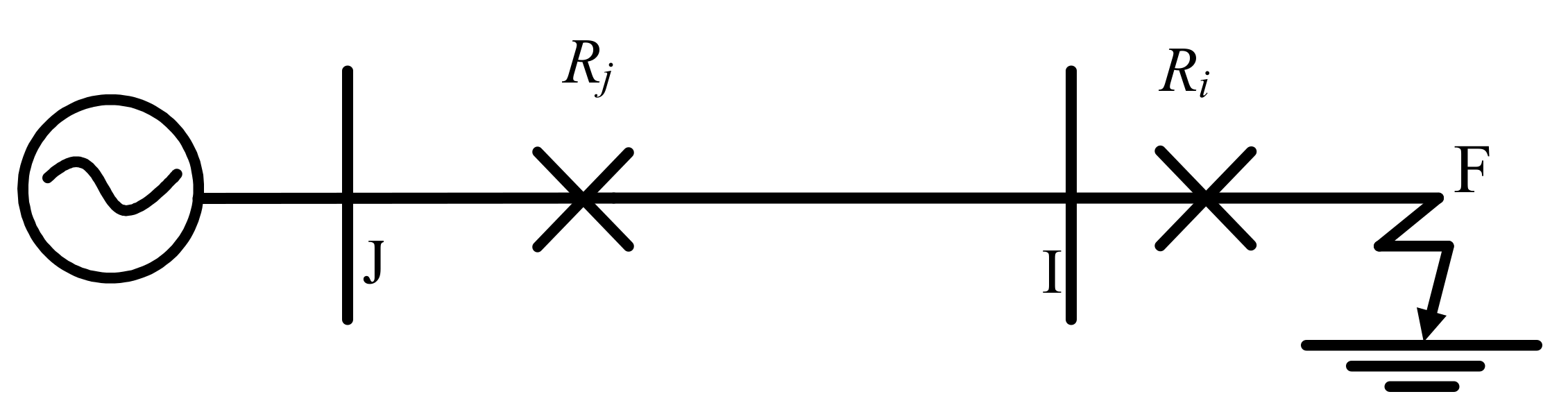
2. Problem Formulation of the Overcurrent Relay

The coordination of the overcurrent relay is defined as an optimization issue in a multi- or single-source loop system. Nonetheless, the coordination issue has an objective function and limitations that should fulfill the distinct constraints:

$$\min f={\displaystyle \sum }_{j=1}^n{w}_j{T}_{j,k}$$

(1)

where the parameters $w_j$ and $T_{j,k}$ are the weight and operating time of the relay, respectively. For all the relays, $w_j=1$ [33]. Therefore, the characteristic curve for operating relay $R_i$ can be chosen from a portion of the selectable decision of IEC norms and could be characterized as:

$$T_{op}=TM{S}_i\left(\frac{\alpha }{{\left(\frac{I{f}_j}{I{p}_j}\right)}^k-1}\right)$$

(2)

where $\alpha$ and $k$ are steady parameters which characterize the relay characteristics and are expected to be $\alpha =0.14$ and $k=0.02$ for normal inverse type relay. The factors $TM{S}_i$ and $I{p}_j$ are the time multiplier setting and pickup current of the $ith$ relay, respectively, while $I{f}_i$ is the fault current flowing through relay $R_i$.

$$PSM=\frac{I_{fj}}{I{p}_j}$$

(3)

where PSM remains for the plug setting multiplier and Ip_j is the primary or main pickup current.

$$T_{op}=TM{S}_i\left(\frac{\alpha }{{\left(PSM\right)}^k-1}\right)$$

(4)

The above issue mentioned in condition (4) is a nonlinear issue in nature. The coordination can be planned as linear programming by considering the plug setting of the relay and the working time of the relays, a linear function of TMS. In linear programming, the TMS is ceaseless while rest of the parameters are steady, so condition (4) moves toward becoming:

$$T_{op}=a_{\rho }(TM{S}_i)$$

(5)

where:

$$a_{\rho }=\frac{\alpha }{{\left(PSM\right)}^k-1}$$

(6)

Hence, the objective function can be formulated as:

$$minf={\displaystyle \sum }_{i=1}^n{a}_{\rho }(TM{S}_i)$$

(7)

Constraints

The total operating time could be minimized under two kinds of constraints, including the constraints of the relay parameter and constraints of coordination. The first constraints contain the limits of TMS while the other constraints are appurtenant to the coordination of the main and secondary relays. The limit on the relay setting parameters necessitates constraints in light of the decisions of relay parameter and design, and the points of confinement can be communicated as follows:

$$TM{S}_i{}^{min}\le TM{S}_i\le TM{S}_i{}^{max}$$

(8)

However, for a reasonable security margin, the pickup current should be lower than the short-circuit current and should be greater than the highest load current simultaneously. The other constraints are convenient for the acclimation of primary and secondary relay operating time. The coordination should be kept in a proper way where the secondary operating time of the relay should be greater than that of the primary relay. If the primary relay fails to clear the fault, the secondary relay should initiate its operation by opening the circuit breaker within a certain interval known as the coordination time interval (CTI). The coordination topology is shown in Figure 1. When a fault F takes place, it is sensed by both relays R_i and R_j. The primary relay responds first, having less operating time than that of the backup relay.

For fault F, beyond bus bar i, relay R_i should respond first to clear the fault. The operating time of R_i is set to 0.1 s. The backup relay should wait for 0.1 s plus the operating time of the circuit breaker at bus bar i and overshoot time of the relay R_j [34]. To maintain selectivity of primary and backup protection and to keep the grading of relay coordination accurate, the operating time of the backup relay (R_j) should always be greater than that of primary relay (R_i) by an amount in which R_i was supposed to have cleared the fault. This time is usually the sum of operating time of R_i and the breaker operating time. The current and voltage wave for the primary/back up pair are shown in Figure 2 for the typical single-end ring main feeder used in the distribution system.

Hence, the coordination constraints could then be defined as:

$$T_j\ge T_i+CTI$$

(9)

where the parameter $T_i$ and $T_j$ are primary and backup relay operating times, respectively.

3. Root Tree Optimization Algorithm

The rooted tree optimization technique is a natural and biological algorithm inspired by the random-oriented movement of roots developed by Labbi Yacine et al. in 2016 [35]. Roots work in a group to find the global optima and the best place to get water, instead of working individually. However, an individual root has a limited capacity and a greater number of roots are based around the place which links the plant with the source of water. To design the algorithm, an imaginary nature of roots should be taken into consideration for their combined decision related to the wetness degree, where the head of the root is located. To find one or more wetness locations by random movement, these roots call other roots to strengthen their presence around that position to become a new starting point for majority of root groups to get to the original place of water that will be the optimal solution. Figure 3 shows the behavior of the roots of a plant that how they search for water to find the best location. The roots which are far or have less wetness degree are replaced by new roots which are oriented randomly. However, the roots which have a greater amount of wetness ratio will preserve their orientation, whereas roots (i.e., solutions) that are far from the water location could be replaced by roots near the best roots of the previous generation.

However, the completion of a maximum number of cycles or generations is the stopping criterion at the end of generations. The solution with best fitness value will be the desired solution. The evaluation of population members is based on a given objective function which is assigned with its fitness value. The candidate with the best solutions is forwarded to next generation while the others are neglected and reimbursed by new group of random solutions in each iteration/generation. The proposed algorithm starts its work by creating an initial population randomly. However, for the RTO algorithm, there are some important parameters that need to be defined regarding how roots start the random movement from the initial population to new population. Those parameters are roots and wetness degree (wd). These two parameters can give the suggested solution and fitness value to the rest of the population. In this work, the RTO algorithm is used to find the optimal solution for the relay coordination problem within a power system. The suggested procedure has an extraordinary exploration ability and merging promptness in contrast with other methodology. This distinguishing property makes the populace individual from RTO more discriminative in locating the ideal result compared to that of another developmental method. The primary point of this paper is to locate the ideal estimations of TMS, keeping in mind the end goal to limit the aggregate working time of OCRs under a few requirements like relay settings and backup constraints.

3.1. The Rate of the Root (R_n) Nearest to the Water

The term rate here represents those roots which are a member of the total population that gather around the wetter place. This root will be next in line to that root where wetness is weaker than that of the previous generation. The fresh population of the nearest root according to wetness condition can be defined as:

$$x^n\left(i,it+1\right)=x_{it}^b+\frac{\left(k_1*w_{di}*randn*l\right)}{n*it}$$

(10)

where $it$ is the current step of the iteration, $x^n\left(i,it+1\right)$ is the fresh member for the next iteration, i.e., $\left(it+1\right)$. The best solution achieved from the previous generation can be represented by $x_{it}{}^b$, while the parameters $k_1, N,i, \mathrm{and} l$ represent the adjustable parameter, population scale number, and upper limit, respectively, and $randn$ is a normal random number having a value between −1 and 1.

3.2. The Rate of the Continuous Root (R_c) in Its District

It is the root which has greater wetness ratio and moves forward from the previous generation. The new population of the random root is expressed as follows:

$$x^n\left(i,it+1\right)=x_{it}^b+\frac{\left(k_2*w_{di}*randn*l\right)}{n*it}*\left(x^b\left(it\right)-x\left(i,it\right)\right)$$

(11)

whereas $k_2$ is the adjustable parameter while $x\left(it\right)$ is the iteration for the previous candidate at iteration it and randn is a random number that has a range between 0 and 1.

3.3. Random Root Rate (R_r)

In this case, the roots spread randomly to find the best location of water to achieve the maximum rate of getting the global solution. The roots with less ratio of wetness degree are also replaced from the last generation. In this step, a new population calculated for a random root could be expressed as:

$$x^n\left(i,it+1\right)=x_{r}it+\frac{\left(k_3*w_{di}*randn*l\right)}{it}$$

(12)

where the parameter $x_r$ is the candidate which is selected randomly from the previous generation with an adjustable parameter $k_3$.

3.4. The Step Root Tree Algorithm

The steps of this algorithm can be compiled as follows:

Step 1:

In this step, the initial generation is created randomly and is composed of N members with the variable limits in the research location with induce numerical values of R_n, R_r, and R_c rates.

Step 2:

In the second step, all population members are measured based on their respective wd for the maximum and minimum objective function:

$$w_{di}= \{\begin{array}{cc}\frac{f_i}{\max \left(f_i\right)}& \mathrm{For}\mathrm{the}\mathrm{maximum}\mathrm{objective}\hfill \\ 1-\frac{f_i}{\max \left(f_i\right)}& \mathrm{For}\mathrm{the}\mathrm{minimum}\mathrm{objective}\hfill \end{array} i=1,2,\dots , N$$

(13)

Step 3:

The new population is created and replacement of the member is done according to the wetness ratio of R_n, R_r, and R_c. Equations (10)–(12) are used for a candidate having the smallest value until the one with the same wetness ratio is achieved.

Step 4:

In this step, the meeting criteria are satisfied to display an optimal result with the best fitness value. Otherwise there is a return to Step 2.

3.5. Implementation of the RTO Algorithm for the OCR Coordination Problem

Step 1:

Define the input parameter that includes TMS, the maximum number of iterations, population size, and the adjustable parameter (i.e., different rate values of R_n, R_r, and R_c).

Step 2:

In this step, the population is initially generated with respect to the relay bounding. These individuals must be a feasible candidate solution that satisfies the relay operating constraints.

Step 3:

Measure the fitness value of each candidate $x_b$ in the population, with the help of Equation (10). Additionally, an evaluation of wetness ratio is done in this step for each candidate.

Step 4:

In this step, the comparison is done between the best fitness values of candidates $\left(x_b{}^{best}\right)$ of the individual population.

Step 5:

Computation of new candidates can be done using Equations (10)–(12).

$$X_b\left(i+1\right)=\left(X_{bi,r}+w_{di}+k_3\right)\frac{randn\left(X_{bi,max}-X_{bi,min}\right)}{it}\mathrm{for}i=1,\dots ,R_r\times n$$

$$X_b\left(i+1\right)=\left(\left(X^{best}{}_b\left(i\right)+w_{di}+k_1\right)\right)\frac{rand\left(X_{bi,max}-X_{bi,min}\right)}{n*it}\mathrm{for}i=(R_r*n)+1,\dots ,n\times (R_r+R_n)$$

$$X_b\left(i+1\right)=\left(\left(X_b\left(i\right)+w_{di}+k_2\right)\right)randn\left(X^{best}{}_b-X_{bi,min}\right) \mathrm{for}i=\left(R_n+R_c\right)\times n+1,\dots ,n$$

(14)

where X_bi,r is the individual that is randomly selected from the current population, n is the population size, X_bi,max, and X_bi,max are upper and lower parameter limits, respectively, and i is the number of iterations.

Step 6:

If the number of iterations reaches the maximum, then go to Step 7. Otherwise, go to Step 3.

Step 7:

The candidates that generate the latest $x_b{}^{best}$ is the optimal TMS of each relay with the minimum total operating time that is the objective function.

The implementation and pseudocode of RTO for solving the coordination problem of OCR is depicted in Figure 4 and Algorithm 1.

Algorithm 1. The structure of the new rooted tree algorithm [35].

Algorithm RTO   Begin   // Initialization:   Set the rates Rn, Rr and Rc parameters   Give the maximum number of iterations: MaxIte, and the population scale: the RTO size   Set iteration counter it = 1   Generate the initial population X(1) randomly within the search range of (Xmin, Xmax)   // Loop   Repeat   Evaluate the wdi for each root // wd: Fitness, root: Individual   Reorder the population according to the witness degree   Identify the candidate according to the wetness place   Xbest // the global best in the whole population   For i = 1 to Rr the RTO size do   Selected individual Xr it randomly from the current population   Xi (it + 1) = Xr (it) + k1* wdi * randn * |Xmax + Xmin|/it   End for   For i= Rr * the RTO size +1 to (Rr+Rn) the RTO size do   Xi(it+1) = Xbest + k3* wdi *randn * | Xmax + Xmin |/(it theRTOsize)   End for   For i = (1 − Rc) the RTO size +1 to the RTO size do   Xi (it+1) = Xi (it) +k1* wdi *rand * (Xbest − Xi (it))   End for   Update Xbest   it = it + 1   Until for a stop criterion is not satisfied // & it <MaxIte   End

4. Results and Discussion

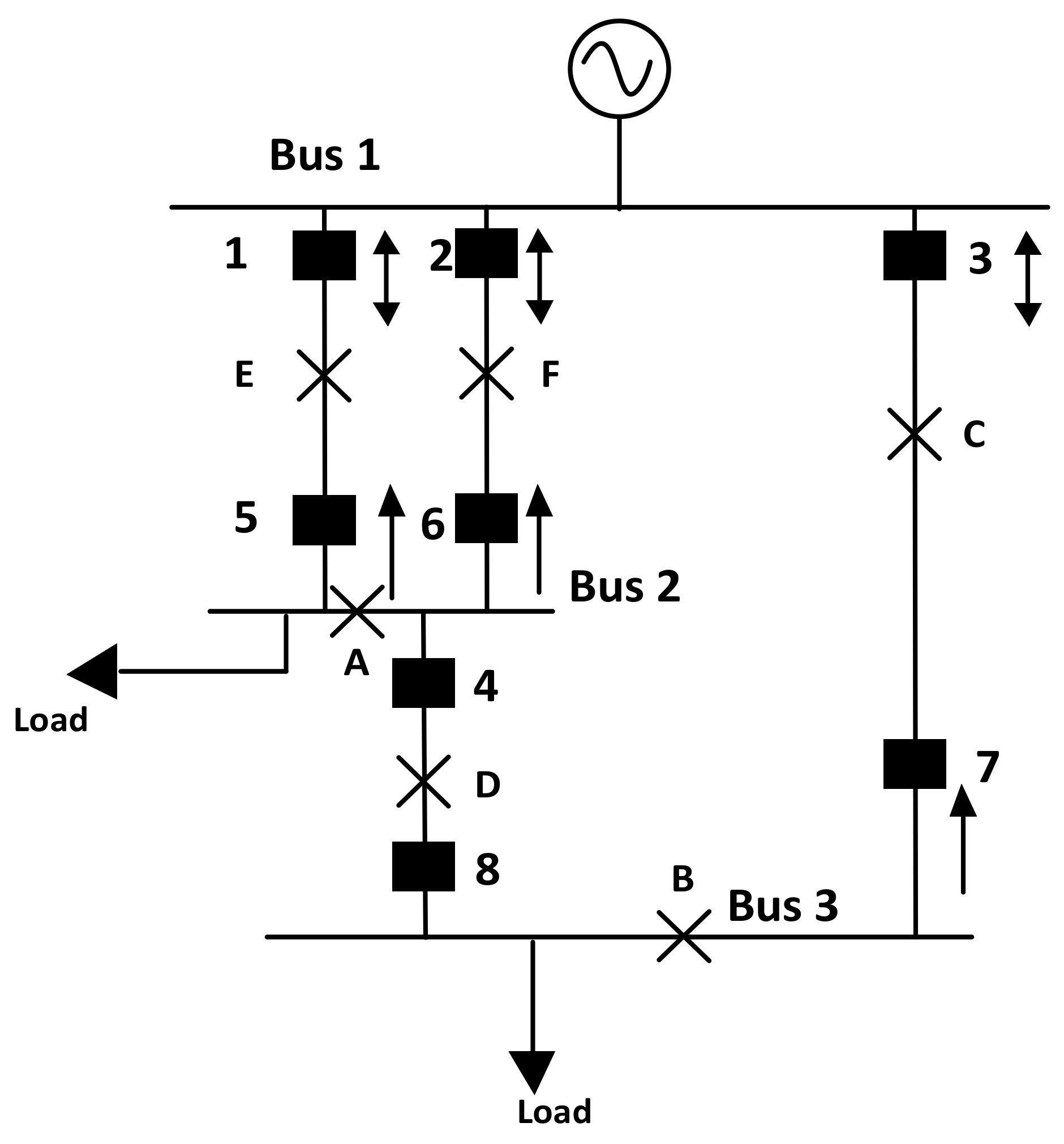
In this segment, a legitimate program has been created in MATLAB software to locate the optimum value of OCR in a single- and multi-loop distribution system utilizing RTO. The productivity and execution of RTO were tried for the distinctive single- and multi-loop system, and it was discovered that the RTO gives the most tasteful and best solution in all the contextual analyses. Three contextual analyses have been viewed. The system details of all contextual investigations could be found in [36,37,38,39]. In each case study, the following RTO parameters were used. The comprehensive explanation of the problem formulation and application of RTO to find the optimal solution is presented for all case studies. For the purpose of this study, population size = 50 and the maximum number of iteration = 200.

4.1. Case Study 1

Figure 5 shows a multi-loop system having eight overcurrent relays. The configuration and combustion of the primary and secondary relay pair models depend upon the location of the fault current in different feeders. In this combination, six different fault locations are taken into consideration. The aggregate fault current and the essential reinforcement relationship of the relay for the six fault focuses are given in

Table 1. Total fault current and primary/backup relationships of relays for Case 1.

Fault Point	T. Fault Current	Primary Relay	Backup Relay
A	2330	1, 2, 8	-, -, 3
B	1200	3, 4	-, 1, 2
C	1400	3, 7	-, 4
D	1400	4, 8	1, 2, 3
E	2800	1, 5	-, 8
F	2800	2, 6	-, 8

- Indicates no backup relay.

. All relays have a plug setting of 1 and a CT ratio of 100:1.

Table 2. $a_{\rho }$ constants and relay currents for Case 1.

Fault Point		Relay
		1	2	3	4	5	6	7	8
A	Irelay	10	10	3.3	-	-	-	-	3.3
	$a_{\rho }$	2.971	2.971	5.749	-	-	-		5.749
B	Irelay	3.45	3.45	5.1	6.9	-	-	-	-
	$a_{\rho }$	5.584	5.584	4.227	3.551	-	-	-	-
C	Irelay	2	2	10	4	-	-	4	-
	$a_{\rho }$	10.035	10.035	2.971	4.9804	-	-	4.9804	-
D	Irelay	5	5	4	10	-	-	-	4
	$a_{\rho }$	4.281	4.281	4.9804	2.971	-	-	-	4.9804
E	Irelay	20	6	2	-	8	-	-	2
	$a_{\rho }$	2.267	3.837	10.035	-	3.297	-	-	10.035
F	Irelay	6	20	2	-	-	8	-	2
	$a_{\rho }$	3.837	2.267	10.035	-	-	3.297	-	10.035

shows the current seen by relays and the a_ρ constant for various faults.

4.1.1. Mathematical Modelling of the Problem Formulation

In this case, eight variables had been taken into consideration (i.e., the TMS of eight relays), eight constraints due to bounds on relay operating time (or bounds on the TMS of relays), and nine constraints due to coordination criteria. The duplex of the proposed problem will have 17 variables and 8 constraints. In order to validate the efficiency of RTO, the CTI ratio of 0.6 s and minimum operating time (MOT) of the relay was taken as 0.1 s. The TMS of all the eight relays are x1–x8.

The problem for optimization can be demonstrated as:

$$minz=28.975x_1+28.975x_2+37.736x_3+11.502x_4+3.297x_5+3.297x_6+4.9807x_7+30.7994x_8$$

(15)

The constraints owing to the MOT of the relays are:

$$2.971x_1\ge 0.1$$

(16)

$$2.971x_2\ge 0.1$$

(17)

$$5.584x_3\ge 0.1$$

(18)

$$4.980x_4\ge 0.1$$

(19)

$$3.297x_5\ge 0.1$$

(20)

$$3.297x_6\ge 0.1$$

(21)

$$4.980x_7\ge 0.1$$

(22)

$$10.035x_8\ge 0.1$$

(23)

Hence, the constraints mentioned in Equations (18), (19), (22), and (23) violate the constraints of the minimum value of the (TMS). Hence, these constraints are reconstructed as:

$$x_3\ge 0.025$$

(24)

$$x_4\ge 0.025$$

(25)

$$x_7\ge 0.025$$

(26)

$$x_8\ge 0.025$$

(27)

The constraints owing to the coordination of relays with CTI taken as 0.6 are:

$$5.749x_3-5.749x_8\ge 0.6$$

(28)

$$5.584{\mathrm{x}}_1-3.551{\mathrm{x}}_4\ge 0.6$$

(29)

$$5.584{\mathrm{x}}_2-3.551{\mathrm{x}}_4\ge 0.6$$

(30)

$$4.980{\mathrm{x}}_4-4.980{\mathrm{x}}_7\ge 0.6$$

(31)

$$4.281{\mathrm{x}}_1-2.971{\mathrm{x}}_4\ge 0.6$$

(32)

$$4.980{\mathrm{x}}_3-4.980{\mathrm{x}}_8\ge 0.6$$

(33)

$$10.035{\mathrm{x}}_8-3.297{\mathrm{x}}_5\ge 0.6$$

(34)

$$10.035x_8-3.297{\mathrm{x}}_6\ge 0.6$$

(35)

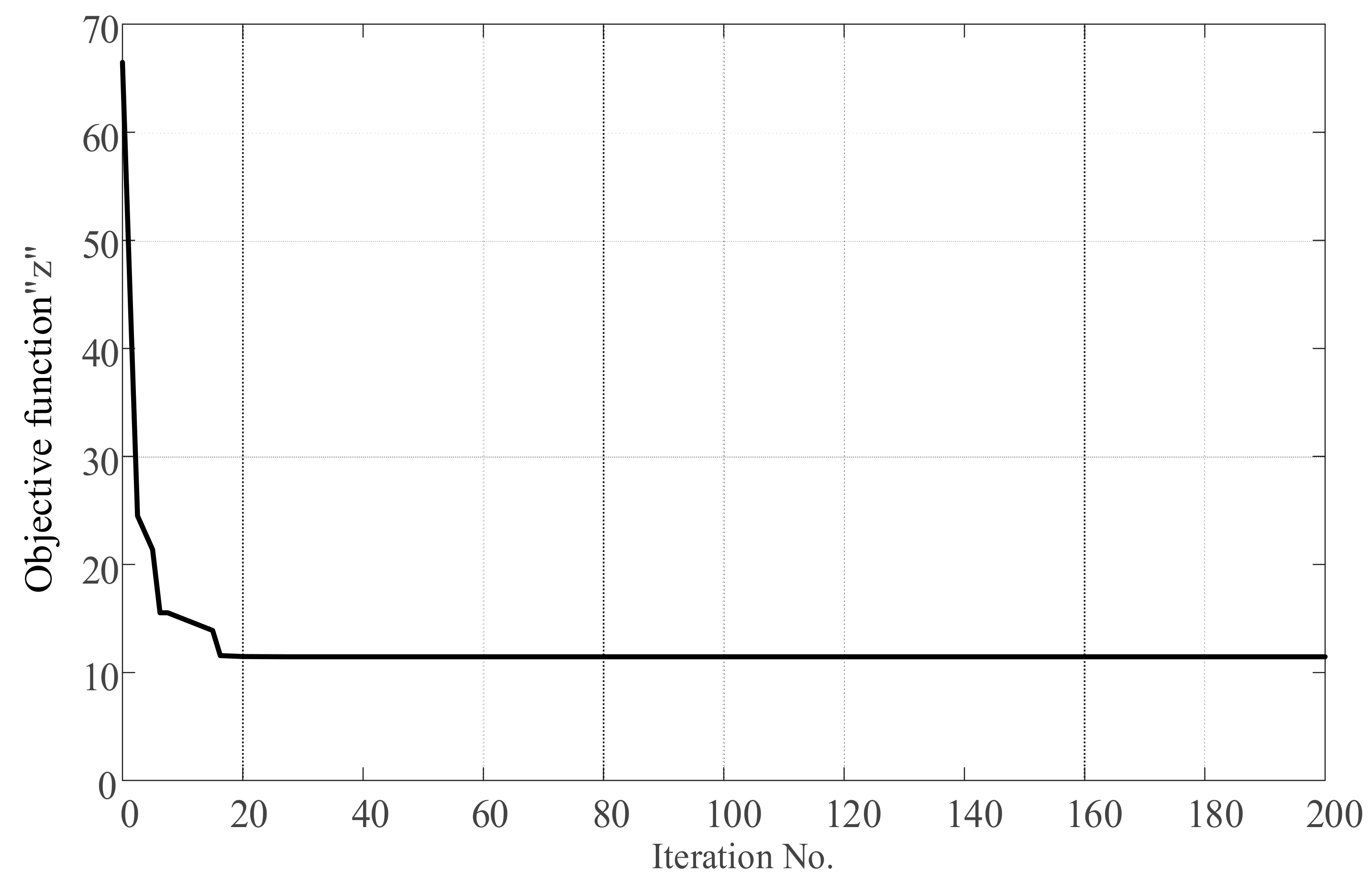
4.1.2. Application of RTO

As discussed in Section 2, to apply RTO to this problem, the objective function was first converted into an unconstrained optimization problem by integrating the relay constraint into the objective function. The constraints pertaining to the MOT of the relay have the ability to alarm the lower bounds of the RTO. The TMS values of all the relays varies from 0.025 to 1.2. The constraint owing to the MOT of the relay was taken care of defining the lower bounds of the variable in RTO. The lower and upper limit of all TMS of the relay is considered as 0.025 to 1.2. The constraints pertaining to coordination of the relay depicted by Equations (28)–(35) were incorporated in the objective function by means of a penalty scheme. In order to justify the RTO, a population size of 50 (i.e., candidate solutions, eight designed variables x₁ to x₈, and 200 iterations as meeting criterion) has been assigned to the coordination problem. The population was conveyed to the fitness function and the proceeding values of the objective function are perceived. As the objective function is of the minimization type, the lowest fitness value of the objective function is considered is the best solution among the population size. After running 200 iterations, the optimum values are shown in

Table 3. Optimal TMS for Case 1.

TMS	GA [36] (≥0.6)	RTO (≥0.6)
TMS 1	0.2975	0.2521
TMS 2	0.2975	0.2521
TMS 3	0.2270	0.2000
TMS 4	0.1730	0.1510
TMS 5	0.0607	0.0303
TMS 6	0.0607	0.0303
TMS 7	0.0402	0.0250
TMS 8	0.1129	0.0800
Top (z)	31.883	26.681

. Table 3 shows the optimal TMS values achieved by the proposed RTO method for this case and has been compared with the literature. Figure 6 shows the objective function values achieved during the course of the simulation for the best candidate solution in each iteration, and this figure shows that the convergence rate is faster and achieves satisfactory results in less iterations compared to other techniques cited in the literature. This figure also shows that R_n = 0.4, R_r = 0.3, and R_c = 0.3 are the feasible values for the RTO technique. These parameter values are used for the rest of the case studies presented in this paper as it gives an optimal solution compared with other adjustable parameters of the RTO algorithm. Figure 7 shows the graphical representation of the optimized total operating time, Top (z), and demonstrates that the total operating time is minimized up to the optimum value. The optimal value of objective is found to be 26.681 s by considering a CTI of 0.6 s, which is obtained in a fewer number of simulations.

The values depicted in Table 3 illustrate that the RTO technique gives an ideal and best-streamlined aggregate working time (i.e., total operating time) up to the ideal optimum value. The optimum values guarantee that the relay will operate in the minimum time to detect a fault at any location. All the optimal values obtained by RTO satisfy all the coordination constraints.

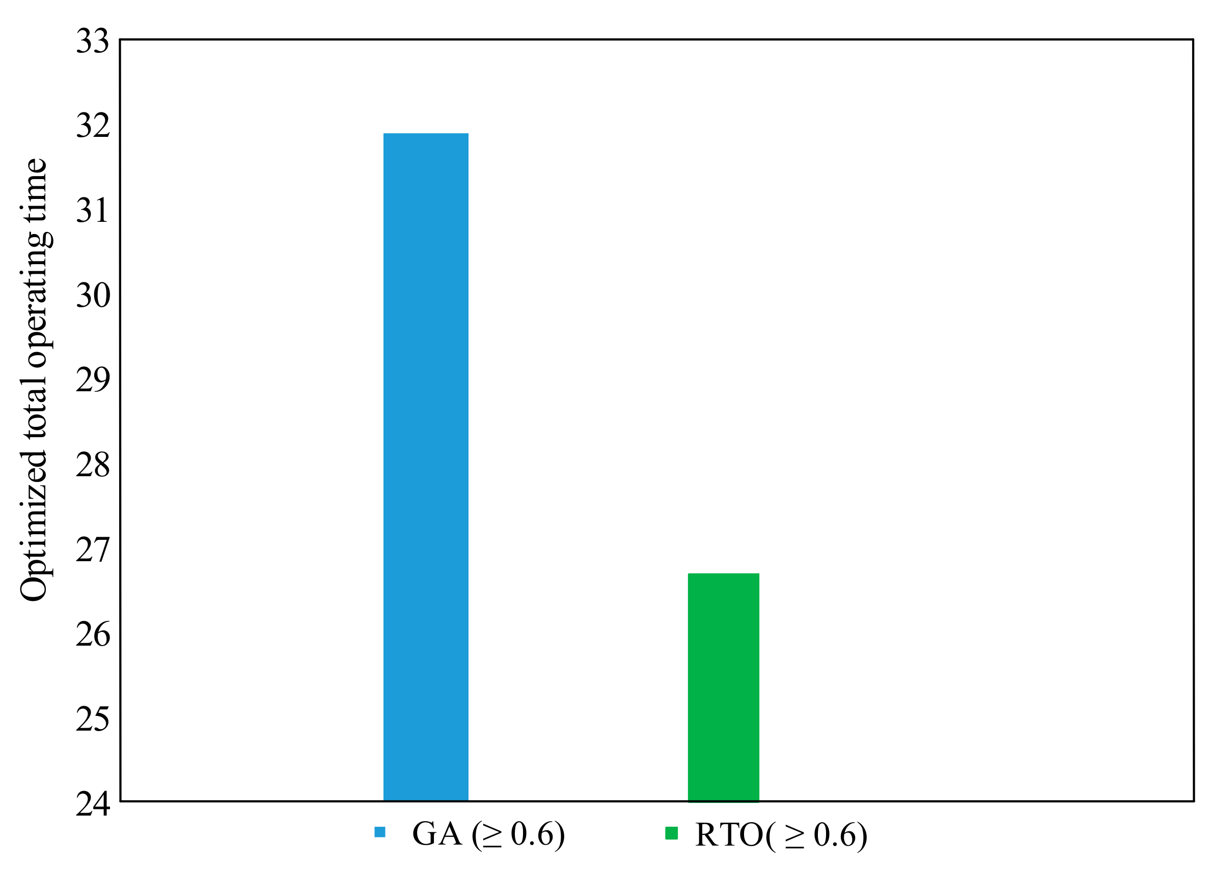
4.1.3. Comparison of RTO with the GA Algorithm

The results obtained by using the RTO algorithm are compared with the genetic algorithm, as given in Table 3. The RTO outperforms the genetic algorithm for obtaining the optimum TMS values and gives the advantage of 5.20198 s over the GA with the same initial conditions as supposed for this case study. The proposed RTO performs outstandingly over GA, gives an advantage in total net time gain, minimizes the total operating time up to the optimum value, and maintains proper coordination during a fault condition. In this condition, the results obtained by RTO for all the relays will satisfy the coordination constraints. Furthermore, no violation has been found regarding the coordination constraints.

4.2. Case Study 2

A multi-loop system, as appeared in Figure 8, with six overcurrent relays and with inconsequential line charging admittances are considered. Four faults are taken into consideration in the midst of the lines, i.e., A, B, C, and D.

4.2.1. Mathematical Modelling of the Problem Formulation

Table 4. Line data for Case 2.

Line	Impedance (Ω)
1 and 2	0.08 +j1
2 and 3	0.08 + j1
1 and 3	0.16 + j2

demonstrates the line information of the given system. The primary/backup pair of relays for the system are shown in

Table 5. Primary and backup relationships of the relays for Case 2.

Fault Point	Primary Relay	Backup Relay
A	1, 2	-, 4
B	3, 4	1, 5
C	5, 6	-, 3
D	3, 5	1, -

- Indicates no backup relay.

. For this delineation, four fault areas are taken, as shown in Figure 8. The CT proportions and plug setting are given in

Table 6. CT ratios and plug settings of the relays for Case 2.

Relay	CT Ratio	Plug Setting
1	1000/1	1
2	300/1	1
3	1000/1	1
4	600/1	1
5	600/1	1
6	600/1	1

. For various fault areas, the current seen by relays and the a_ρ constant are given in

Table 7. $a_{\rho }$ constants and relay currents for Case 2.

Fault Point		Relay
		1	2	3	4	5	6
A	Irelay	6.579	3.13	-	1.565	1.565	-
	$a_{\rho }$	3.646	6.065	-	15.55	15.55	-
B	Irelay	2.193	-	2.193	2.193	2.193	-
	$a_{\rho }$	8.844	-	8.844	8.844	8.844	-
C	Irelay	1.096	-	1.096	-	5.482	1.827
	$a_{\rho }$	75.91	-	75.91	-	4.044	11.539
D	Irelay	1.644	-	1.644	-	2.741	-
	$a_{\rho }$	13.99	-	13.99	-	6.872	-

.

In this representation, the entire number of constraints that arise are 11. Six constraints are attributable to limits on relay working time, and five constraints are by reason of coordination criteria. The MOT of each relay is 0.1, and the CTI is considered as 0.3 s. The TMSs of all six relays are x₁–x₆.

The problem for optimization can be demonstrated as:

$$minz=102.404x_1+6.0651x_2+98.758x_3+24.403x_4+35.319x_5+11.539x_6$$

(36)

The constraints owing to the MOT of the relays are:

$$3.646x_1\ge 0.1$$

(37)

$$6.055x_2\ge 0.1$$

(38)

$$8.844x_3\ge 0.1$$

(39)

$$8.844x_4\ge 0.1$$

(40)

$$4.044x_5\ge 0.1$$

(41)

$$11.539x_6\ge 0.1$$

(42)

Hence, the constraints mentioned in Equations (38)–(42) violate the constraints of the minimum value of the TMS. Hence, these constraints are reconstructed as:

$$x_2\ge 0.025$$

(43)

$$x_3\ge 0.025$$

(44)

$$x_4\ge 0.025$$

(45)

$$x_5\ge 0.025$$

(46)

$$x_6\ge 0.025$$

(47)

The constraints owing to the coordination of relays with the CTI taken as 0.3 are:

$$15.55x_4-6.065x_2\ge 0.3$$

(48)

$$8.844x_1-8.844x_3\ge 0.3$$

(49)

$$8.844x_5-8.844x_4\ge 0.3$$

(50)

$$75.91x_3-11.53x_6\ge 0.3$$

(51)

$$13.998x_1-13.998x_3\ge 0.3$$

(52)

4.2.2. Application of RTO

The objective function was evaluated using the proposed RTO calculation with same parameters elucidated from delineation 1. The optimal values of TMS gained are given in

Table 8. Optimal TMS for Case 2.

TMS	CGA [37] (≥0.3)	FA [38] (≥0.3)	CFA [38] (≥0.3)	CPSO [40] (≥ 0.3)	RTO (≥0.3)
TMS 1	0.0765	0.027	0.027	0.0589	0.0590
TMS 2	0.034	0.130	0.221	0.0250	0.0250
TMS 3	0.0339	0.025	0.025	0.0250	0.0250
TMS 4	0.036	0.025	0.025	0.0290	0.0290
TMS 5	0.0711	0.025	0.029	0.0630	0.0650
TMS 6	0.0294	0.489	0.363	0.0250	0.0250
Top (z)	15.88	16.25	14.39	11.87	11.93

, which shows that the RTO algorithm gives ideal and best values and that it optimized the total operating time to optimal values. The optimal values ensure that the relay will take the least possible time in the system for a fault at any area. The time taken by Relay 1 to work is the base for a fault at point A and will set aside the most noteworthy time for a relay at point C. This is alluring in light of the fact that, for a fault at point A, relay 1 is first to work while, for a fault at point C, Relay 6 should get first chance to work if it fails. Relay 3 should take over tripping action and, if Relay 3 in a similar manner fails to work, then Relay 1 ought to expect control over the tripping action. The objective function value achieved over the span of the simulation for the best applicant arrangement in every cycle is shown in Figure 9. This demonstrates that the convergence is speedier and obtained a satisfactory value in fewer iterations. The optimum value of the objective function is observed to be 11.93 by considering CTI being taken as 0.3 s. Figure 10 demonstrates the optimized total operating time accomplished by the proposed algorithm with other methods mentioned in the literature

4.2.3. Comparison of RTO with Other Algorithms

To evaluate the execution of the proposed RTO algorithm, this technique was compared with the other mathematical and evolutionary techniques such as the CGA, FA, CFA, and CPSO technique accessible in the literature, as shown in Table 8. The RTO outmatched the CGA, FA, and CFA given the total net gain of times and gives advantages of 3.95, 4.32, and 2.46 s over these methods, respectively. However, in the case of CPSO, this technique almost converges to the same optimum solution as obtained by using the RTO with more computational effort. Furthermore, the RTO algorithm is better than the other techniques mentioned in the literature in terms of the nature of the results. Convergence representation and less number of iterations is required to get the ideal and best result.

4.3. Case Study 3

A parallel distribution system that is sustained from a singular end with seven overcurrent relays is shown in Figure 11. The CT ratio and PS of the relays are shown in

Table 9. CT ratios and plug settings of the relays for Case 3.

Relay	CT Ratio	Plug Setting
1	1000/1	0.8
2	1000/1	0.8
3	1000/1	0.8
4	1000/1	0.8
5	1000/1	0.8
6	1000/1	0.8
7	500/1	0.5

. Four faults streams are constrained in the midst of the lines, i.e., A, B, C, and D. The primary/backup pair of relays for the given system are shown in

Table 10. Primary and backup relationships of the relays and maximum fault current for Case 3.

Fault Point	Primary Relay	Backup Relay	T. Fault Current (A)
A	1	-	6579
	4	2	939
B	3	1	2193
	4	5	1315.5
C	5	-	3289.5
	6	3	1096.5
D	7	3	1315.8 through relays 3 and 5
	-	5	2631.6 through relay 7

.

4.3.1. Mathematical Modelling of the Problem Formulation

For this case, the total number of constraints is 12. Seven imperatives arise as a result of the points of confinement of the relay action, and five prerequisites arise due to the coordination condition. The MOT of each relay is 0.1 s. The CTI is considered as 0.2 s. The TMS values of all the relays is x₁–x₇. For different fault regions, the current seen by relays and the a_ρ constant are given in

Table 11. $a_{\rho }$ constants and relay currents for Case 3.

Fault Point		Relay
		1	2	3	4	5	6	7
A	Irelay	8.223	1.1737	-	2.347	-	-	-
	$a_{\rho }$	3.252	43.776	-	8.159	-	-
B	Irelay	2.741	-	5.482	3.288	1.644	-	-
	$a_{\rho }$	6.872	-	4.0444	5.811	14.01	-	-
C	Irelay	-	-	2.741	-	4.111	1.370	-
	$a_{\rho }$	-	-	6.872	-	4.881	22.165	-
D	Irelay	-	-	3.289	-	3.289	-	5.263
	$a_{\rho }$	-	-	5.809	-	5.809	-	4.145

.

The problem for optimization can be demonstrated as:

$$minz=10.124x_1+43.776x_2+16.725x_3+13.97x_4+24.703x_5+22.165x_6+4.145x_7$$

(53)

The constraints owing to the MOT of the relays are:

$$3.252x_1\ge 0.1$$

(54)

$$43.776x_2\ge 0.1$$

(55)

$$4.044x_3\ge 0.1$$

(56)

$$5.811x_4\ge 0.1$$

(57)

$$4.881x_5\ge 0.1$$

(58)

$$22.165x_6\ge 0.1$$

(59)

$$4.145x_7\ge 0.1$$

(60)

Hence, the constraints mentioned in Equations (55)–(60) violate the constraints of the minimum value of the TMS. Hence, these constraints are reconstructed as:

$$x_2\ge 0.025$$

(61)

$$x_3\ge 0.025$$

(62)

$$x_4\ge 0.025$$

(63)

$$x_5\ge 0.025$$

(64)

$$x_6\ge 0.025$$

(65)

$$x_7\ge 0.025$$

(66)

The constraints owing to the coordination of relays with the CTI taken as 0.2 are:

$$43.77x_2-8.159x_4\ge 0.2$$

(67)

$$6.872x_1-4.044x_3\ge 0.2$$

(68)

$$14.01x_5-5.811x_4\ge 0.2$$

(69)

$$22.165x_3-6.872x_6\ge 0.2$$

(70)

$$5.809x_3-4.145x_7\ge 0.2$$

(71)

4.3.2. Application of RTO

The objective function was solved by the proposed RTO with vague parameters. The ideal estimations of TMS and aggregate working time found are shown in

Table 12. Optimal TMS for Case 3.

TMS	SM [39] (≥0.2)	RTO (≥0.2)
TMS 1	0.23829	0.0852
TMS 2	0.12	0.0250
TMS 3	0.36036	0.0953
TMS 4	0.0319	0.0250
TMS 5	0.02773	0.0250
TMS 6	0.025	0.0250
TMS 7	0.08	0.0250
Top (z)	15.7068	5.1756

. They similarly show the comparative delayed consequence of RTO with other metaheuristic and numerical procedures in the literature. In this depiction, no encroachment and miscoordination of the relays have been found. The time taken by relay R1 to work is the least for a fault at point C and is most extreme for a fault at point A. This is attractive on the grounds that, for a fault at point C, relay 1 is the first to work. Meanwhile, for a fault at point A, relay 7 ought to get the principal opportunity to work. On the off chance that it neglects to work, relay 4 should assume a control tripping activity. If relay 4 likewise neglects to work, relay 1 should assume control over the tripping activity at that point. The values are given in Table 12 ensure that the relays will work at any rate possible time for a fault whenever in the system. The objective value acquired over the span of the simulation for the best candidate course of action in each iteration is shown in Figure 12, which exhibits that the convergence is faster and get the best qualities in a lesser number of iterations. Additionally, the RTO outmatched the simplex method for this case and obtained an agreeable and better outcome compared to the simplex technique. The graphical image of the improved aggregate working time appears in Figure 13 and shows that the total operating time is streamlined up to the ideal and optimum value when compared to the simplex method, as mentioned in the literature.

4.3.3. Comparison of RTO with the Simplex Method

The results found using the RTO are differentiated, and the results procured by the simplex method are shown in Table 12. The RTO outmatch the simplex method in getting the optimal values of TMS and in an aggregate net gain of times. It gives a benefit of 10.5312 s over the simplex method, with the same starting parameters gathered for this contextual investigation. This gain in all out net time gain is adequate given that it is a small system. For all the ideal and optimal values for TMS, the RTO performed exceptionally compared to the simplex method, in terms of complete net time gain. Furthermore, it limits the aggregate working time up to optimal value and will keep up appropriate coordination even in a fault condition. For all the coordination conditions, the optimal value acquired by RTO for all the relays will fulfill the coordination limitations. Additionally, no infringement has been discovered with respect to the coordination requirements.

5. Conclusions

This paper suggested an RTO algorithm which simulates plant roots searching for water under the ground. The aforementioned RTO technique involved some parameters for tuning and, thus, is easy to implement. The coordination problem of the overcurrent relay utilizes the RTO algorithm for different test systems to assess the execution of the proposed RTO algorithm. The competence of the proposed RTO algorithm has been confirmed and tried through its application on various single- and multi-loop systems by analyzing its superiority and contrasting its execution with the CFA, FA, CPSO, CGA, GA, and the simplex method published algorithms. The simulation results of the RTO algorithm efficiently minimize all three models of the problem. The performance of the RTO can be seen from the optimized minimum objective function values and TMS, of each relay in the systems achieved by RTO for each case studies. In case 1 the objective function value is minimized up to optimum value by RTO and gives an advantage in total net gain in time of 5.20198 s over GA. while in case 2 and 3 the RTO gives a total net gain in time 3.95 s, 4.32 s, 2.46 s, and 10.5312 s over CGA, FA, CFA, and simplex method. The RTO algorithm gives a new seeking approach for elucidation, as one of its qualities is the extensive field of research attributable to the activities of the roots. The simulation results uncover the predominance of the proposed RTO algorithm in taking care of the overcurrent relay coordination problem. In future work, RTO will be applied to solve the problem of overcurrent relay coordination of higher and complex buses in the electrical power system.

References

1. Urdaneta, A.J.; Nadira, R.; Jimenez, L.G.P. Optimal coordination of directional overcurrent relays in interconnected power systems. IEEE Trans. Power Deliv. 1988, 3, 903–911. [Google Scholar] [CrossRef]
2. Birla, D.; Maheshwari, R.P.; Gupta, H.O.; Deep, K.; Thakur, M. Application of random search technique in directional overcurrent relay coordination. Int. J. Emerg. Electr. Power Syst. 2006, 7. [Google Scholar] [CrossRef]
3. Ehrenberger, J.; Švec, J. Directional Overcurrent Relays Coordination Problems in Distributed Generation Systems. Energies 2017, 10, 1452. [Google Scholar] [CrossRef]
4. Ates, Y.; Boynuegri, A.; Uzunoglu, M.; Nadar, A.; Yumurtacı, R.; Erdinc, O.; Paterakis, N.; Catalão, J. Adaptive protection scheme for a distribution system considering grid-connected and islanded modes of operation. Energies 2016, 9, 378. [Google Scholar] [CrossRef]
5. Núñez-Mata, O.; Palma-Behnke, R.; Valencia, F.; Jiménez-Estévez, P.M.G. Adaptive Protection System for Microgrids Based on a Robust Optimization Strategy. Energies 2018, 11, 308. [Google Scholar] [CrossRef]
6. Elrafie, H.B.; Irving, M.R. Linear programming for directional overcurrent relay coordination in interconnected power systems with constraint relaxation. Electr. Power Syst. Res. 1993, 27, 209–216. [Google Scholar] [CrossRef]
7. Aghdam, T.S.; Hossein, K.K.; Hatem, Z. Optimal Coordination of Double-Inverse Overcurrent Relays for Stable Operation of DGs. IEEE Trans. Ind. Inform. 2018. [Google Scholar] [CrossRef]
8. Aghdam, T.S.; Karegar, H.K.; Zeineldin, H.H. Transient Stability Constrained Protection Coordination for Distribution Systems with DG. IEEE Trans. Smart Grid 2017. [Google Scholar] [CrossRef]
9. Ojaghi, M.; Mohammadi, V. Use of Clustering to Reduce the Number of Different Setting Groups for Adaptive Coordination of Overcurrent Relays. IEEE Trans. Power Deliv. 2018, 33, 1204–1212. [Google Scholar] [CrossRef]
10. Braga, A.S.; Saraiva, J.T. Coordination of overcurrent directional relays in meshed networks using the Simplex method. In Proceedings of the 8th Mediterranean Electrotechnical Conference on Industrial Applications in Power Systems, Computer Science and Telecommunications (MELECON’96), Bari, Italy, 16 May 1996; Volume 3. [Google Scholar]
11. Abyaneh, H.A.; Keyhani, R. Optimal co-ordination of overcurrent relays in power system by dual simplex method. In Proceedings of the Australasian Universities Power Engineering Conference (Aupec’95), Nedlands, Australia, 27–29 September 1995; Volume 3. [Google Scholar]
12. Abdelaziz, A.Y.; Talaat, H.E.A.; Nosseir, A.I.; Hajjar, A.A. An adaptive protection scheme for optimal coordination of overcurrent relays. Electr. Power Syst. Res. 2002, 61, 1–9. [Google Scholar] [CrossRef]
13. Laway, N.A.; Gupta, H.O. A method for adaptive coordination of overcurrent relays in an interconnected power system. In Proceedings of the 1993 Fifth International Conference on Developments in Power System Protection, York, UK, 30 March–2 April 1993. [Google Scholar]
14. Sulaiman, M.; Waseem; Muhammad, S.; Khan, A. Improved Solutions for the Optimal Coordination of DOCRs Using Firefly Algorithm. Complexity 2018, 2018, 7039790. [Google Scholar] [CrossRef]
15. Mansour, M.M.; Mekhamer, S.F.; El-Kharbawe, N. A modified particle swarm optimizer for the coordination of directional overcurrent relays. IEEE Trans. Power Deliv. 2007, 22, 1400–1410. [Google Scholar] [CrossRef]
16. Zeineldin, H.H.; El-Saadany, E.F.; Salama, M.M.A. Optimal coordination of overcurrent relays using a modified particle swarm optimization. Electr. Power Syst. Res. 2006, 76, 988–995. [Google Scholar] [CrossRef]
17. Razavi, F.; Abyaneh, H.A.; Al-Dabbagh, M.; Mohammadi, R.; Torkaman, H. A new comprehensive genetic algorithm method for optimal overcurrent relays coordination. Electr. Power Syst. Res. 2008, 78, 713–720. [Google Scholar] [CrossRef]
18. Kim, C.H.; Khurshaid, T.; Wadood, A.; Farkoush, S.G.; Rhee, S.B. Gray Wolf Optimizer for the Optimal Coordination of Directional Overcurrent Relay. J. Electr. Eng. Technol. 2018, 13, 1043–1051. [Google Scholar]
19. Thangaraj, R.; Pant, M.; Deep, K. Optimal coordination of over-current relays using modified differential evolution algorithms. Eng. Appl. Artif. Intell. 2010, 23, 820–829. [Google Scholar] [CrossRef]
20. Bouchekara, H.R.E.H.; Zellagui, M.; Abido, M.A. Optimal coordination of directional overcurrent relays using a modified electromagnetic field optimization algorithm. Appl. Soft Comput. 2017, 54, 267–283. [Google Scholar] [CrossRef]
21. Alipour, M.; Teimourzadeh, S.; Seyedi, H. Improved group search optimization algorithm for coordination of directional overcurrent relays. Swarm Evolut. Comput. 2015, 23, 40–49. [Google Scholar] [CrossRef]
22. Brown, K.; Tyle, N. An expert system for over current protective device coordination. McGraw Edison power system division. In Proceedings of the IEEE Rural Electric Power System Conference, Charleston, SC, USA, April 1986; pp. 20–22. [Google Scholar]
23. Lee, S.J.; Yoon, S.H.; Yoon, M.C.; Jang, J.K. An expert system for protective relay setting of transmission systems. IEEE Trans. Power Deliv. 1990, 5, 1202–1208. [Google Scholar]
24. Decher, G.; Hong, J.-D. Buildup of ultrathin multilayer films by a self-assembly process, 1 consecutive adsorption of anionic and cationic bipolar amphiphiles on charged surfaces. Macromol. Symp. 1991, 46, 321–327. [Google Scholar] [CrossRef]
25. Wang, J.; Trecat, J. RSVIES—A relay setting value identification expert system. Electr. Power Syst. Res. 1996, 37, 153–158. [Google Scholar] [CrossRef]
26. Abyane, H.A.; Faez, K.; Karegar, H.K. A new method for overcurrent relay (O/C) using neural network and fuzzy logic. In Proceedings of the IEEE Region 10 Annual Conference, Speech and Image Technologies for Computing and Telecommunications (TENCON’97), Brisbane, Australia, 4 December 1997; Volume 1. [Google Scholar]
27. Yu, J.; Kim, C.H.; Wadood, A.; Khurshiad, T.; Rhee, S.B. A Novel Multi-Population Based Chaotic JAYA Algorithm with Application in Solving Economic Load Dispatch Problems. Energies 2018, 11, 1946. [Google Scholar] [CrossRef]
28. Farkoush, S.G.; Khurshiad, T.; Wadood, A.; Kim, C.-H.; Kharal, K.H.; Kim, K.-H.; Cho, N.; Rhee, S.-B. Investigation and Optimization of Grounding Grid Based on Lightning Response by Using ATP-EMTP and Genetic Algorithm. Complexity 2018, 2018, 8261413. [Google Scholar] [CrossRef]
29. Park, J.H.; Yu, J.S.; Geem, Z.W. Genetic Algorithm-based Optimal Investment Scheduling for Public Rental Housing Projects in South Korea. Int. J. Fuzzy Log. Intell. Syst. 2018, 18, 135–145. [Google Scholar] [CrossRef]
30. Moon, Y.Y.; Geem, Z.W.; Han, G.-T. Vanishing point detection for self-driving car using harmony search algorithm. Swarm Evolut. Comput. 2018, 41, 111–119. [Google Scholar] [CrossRef]
31. Geem, Z.W.; Yoon, Y. Harmony search optimization of renewable energy charging with energy storage system. Int. J. Electr. Power Energy Syst. 2017, 86, 120–126. [Google Scholar] [CrossRef]
32. Wadood, A.; Kim, C.; Loon, T.K.; Hassan, K.; Farkoush, S.G.; Rhee, S.-B. Optimal Coordination of Directional Overcurrent Relays using New Rooted Tree Optimization Algorithm. In Proceedings of the International Conference on Information, System and Convergence Applications (ICISCA/ICW 2018), Bangkok, Thailand, 31 January–2 February 2018. [Google Scholar]
33. Chattopadhyay, B.; Sachdev, M.S.; Sidhu, T.S. An on-line relay coordination algorithm for adaptive protection using linear programming technique. IEEE Trans. Power Deliv. 1996, 11, 165–173. [Google Scholar] [CrossRef]
34. Wadood, A.; Kim, C.-H.; Farkoush, S.G.; Rhee, S.B. An Adaptive Protective Coordination Scheme for Distribution System Using Digital Overcurrent Relays. Korean Inst. Illum. Electr. Install. Eng. 2017, 5, 53. [Google Scholar]
35. Labbi, Y.; Attous, D.B.; Gabbar, H.A.; Mahdad, B.; Zidan, A. A new rooted tree optimization algorithm for economic dispatch with valve-point effect. Int. J. Electr. Power Energy Syst. 2016, 79, 298–311. [Google Scholar] [CrossRef]
36. Bedekar, P.P.; Bhide, S.R.; Kale, V.S. Optimum coordination of overcurrent relays in distribution system using genetic algorithm. In Proceedings of the International Conference on Power Systems (ICPS’09), Kharagpur, India, 27–29 December 2009. [Google Scholar]
37. Bedekar, P.P.; Bhide, S.R. Optimum coordination of overcurrent relay timing using continuous genetic algorithm. Expert Syst. Appl. 2011, 38, 11286–11292. [Google Scholar] [CrossRef]
38. Gokhale, S.S.; Kale, V.S. An application of a tent map initiated Chaotic Firefly algorithm for optimal overcurrent relay coordination. Int. J. Electr. Power Energy Syst. 2016, 78, 336–342. [Google Scholar] [CrossRef]
39. Bedekar, P.P.; Bhide, S.R.; Kale, V.S. Optimum coordination of overcurrent relay timing using simplex method. Electr. Power Compon. Syst. 2010, 38, 1175–1193. [Google Scholar] [CrossRef]
40. Wadood, A.; Kim, C.H.; Khurshiad, T.; Farkoush, S.G.; Rhee, S.B. Application of a Continuous Particle Swarm Optimization (CPSO) for the Optimal Coordination of Overcurrent Relays Considering a Penalty Method. Energies 2018, 11, 869. [Google Scholar] [CrossRef]
Figure 1. A single-end radial distribution system.
Applsci 08 01664 g001
Figure 2. Voltage and current waveform of the primary/backup pair of the relay for the single-end radial system.
Applsci 08 01664 g002
Figure 3. Searching mechanism of the RTO algorithm for searching for the water location [35].
Applsci 08 01664 g003
Figure 4. The flow chart of the RTO algorithm.
Applsci 08 01664 g004
Figure 5. A multi-loop distribution system.
Applsci 08 01664 g005
Figure 6. Convergence characteristic of Case 1 for different adjustable parameters to the RTO algorithm.
Applsci 08 01664 g006
Figure 7. Optimized total operating time with the literature for Case 1.
Applsci 08 01664 g007
Figure 8. A single end-loop distribution system.
Applsci 08 01664 g008
Figure 9. Convergence characteristic representation for Case 2.
Applsci 08 01664 g009
Figure 10. Optimized total operating time with the literature for Case 2.
Applsci 08 01664 g010
Figure 11. A single-end, multi-parallel feeder distribution system.
Applsci 08 01664 g011
Figure 12. Convergence characteristic representation for Case 3.
Applsci 08 01664 g012
Figure 13. Optimized total operating time with the literature for Case 3.
Applsci 08 01664 g013