Frequency-Shifted Optical Feedback Measurement Technologies Using a Solid-State Microchip Laser

1
The State Key Laboratory of Precision Measurement Technology and Instruments, Department of Precision Instrument, Tsinghua University, Beijing 100084, China
2
College of Mechanical Engineering and Applied Electronics Technology, Beijing University of Technology, Beijing 100022, China
3
Beijing Institute of Space Electromechanical, Beijing 100076, China
*
Author to whom correspondence should be addressed.
Appl. Sci. 2019, 9(1), 109; https://doi.org/10.3390/app9010109
Submission received: 29 November 2018
/
Revised: 19 December 2018
/
Accepted: 21 December 2018
/
Published: 29 December 2018
(This article belongs to the Special Issue Precision Dimensional Measurements)
Abstract
:Since its first application toward displacement measurements in the early-1960s, laser feedback interferometry has become a fast-developing precision measurement modality with many kinds of lasers. By employing the frequency-shifted optical feedback, microchip laser feedback interferometry has been widely researched due to its advantages of high sensitivity, simple structure, and easy alignment. More recently, the laser confocal feedback tomography has been proposed, which combines the high sensitivity of laser frequency-shifted feedback effect and the axial positioning ability of confocal microscopy. In this paper, the principles of a laser frequency-shifted optical feedback interferometer and laser confocal feedback tomography are briefly introduced. Then we describe their applications in various kinds of metrology regarding displacement measurement, vibration measurement, physical quantities measurement, imaging, profilometry, microstructure measurement, and so on. Finally, the existing challenges and promising future directions are discussed.
1. Introduction
Laser feedback, also known as laser self-mixing interference, was first applied as a displacement sensor by P.G.R. King in 1963 [1]. It is a physical phenomenon where part of the output laser is reflected or scattered by the external object returning back into the laser resonator to modulate the laser output power, phase, polarization states, and so on [2,3,4,5,6]. Unlike the traditional laser interferometry, laser feedback interference occurs inside the laser resonator, thus making the system concise and auto aligned. In the 1970s, the laser feedback effect of the laser diode (LD) became one of the important research fields due to the development of the optical communication technology. The theoretical system of the LD optical feedback was established by R. Lang, D. Lenstra, W.M. Wang, among others [7,8,9,10]. However, the sensitivity of the LD optical feedback is still not high enough to realize the non-cooperative measurement as the black or high transmission targets.
In 1979, Otsuka reported the external optical feedback of LiNdP4O12 lasers produced using a rotating glass plate [11]. This kind of laser, known as the microchip laser, belongs to the class-B laser, of which the population decays slowly compared with the field [12]. In this case, the feedback signal can be amplified by a gain factor of the ratio γc/γ1, where γc is the damping rate of the laser cavity and γ1 is the damping rate of the population inversion. According to the analysis of classic rate equation, the ratio γc/γ1 of a microchip laser can be high as 106. The ratio is only 103 for an LD laser, and much lower in a gas laser. Therefore, the microchip laser has a high sensitivity compared with other kinds of lasers. It has been applied in various fields, such as displacement sensing [13,14], velocimetry [15], vibrometry [16,17], particle detecting [18], angle measurement [19], and laser parameters measurement [20,21].
Imaging objects inside turbid media [22,23,24,25], such as the biological tissue and scattering liquid, is a challenging problem in many fields. Due to the non-contact, excellent contrast, high-resolution, nonionizing, and noninvasive, optical imaging is currently emerging as a promising method in medical imaging [26] (pp. 1–8) through the use of confocal microscopy [27,28,29], diffuse optical tomography [30,31], fluorescence spectroscopy [32,33], and optical coherence tomography [34,35,36]. For diffuse optical tomography, the penetration depth can be several centimeters into biological tissue, but recovering information from scattered photons is a challenge, and the spatial resolution is on the order of 20% of the imaging depth [26] (p. 249). Most optical imaging methods are based on ballistic photons, which will be rapidly decreased when the penetration depth increases in turbid media; thus, these methods are usually confined to imaging of a few millimeters in biological samples. More recently, the laser optical feedback tomography was demonstrated by Lacot [37], which realizes the surface imaging of a French coin immersed in 1 cm of milk. Combining the technology of confocal tomography and a laser feedback effect, Tan et al. proposed the laser confocal feedback tomography [38,39]. Due to the ultrahigh sensitivity of a solid-state microchip laser to external frequency-shifted feedback, it shows promise towards reaching a greater depth than other methods.
This paper provides an overall review of the research on frequency-shifted optical feedback measurements using a solid-state microchip laser. The remainder of the review is structured as follows. Section 2 reveals the basic principles and experimental setups of the laser feedback interferometer and laser confocal feedback tomography. Section 3 discusses the applications of the laser feedback interferometer in displacement sensing, vibration sensing, particle sensing, liquid evaporation rate measurement, refractive index measurement, and thermal expansion coefficient measurement. In Section 4, the microstructure imaging and measurement, profilometry, lens thickness measurement, and imaging, combined with other technologies, are presented based on the laser confocal feedback tomography. A summary and conclusion are given in Section 5.
2. Experimental Setup and Theoretical Analysis
2.1. Laser Frequency-Shifted Optical Feedback
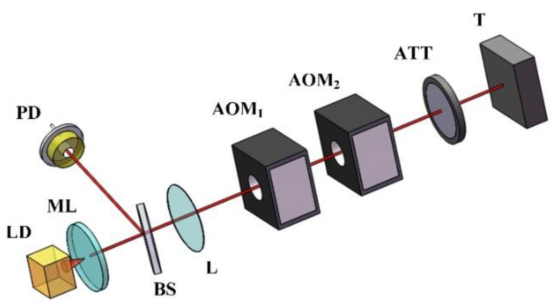
The experimental setup of the laser frequency-shifted optical feedback is shown in Figure 1. A 3 mm × 3 mm × 0.75 mm Nd:YVO4 crystal plate is employed to form a laser resonator with the coating on both surfaces. The left surface is coated to be antireflective at the pump wavelength of 808 nm and highly reflective (R > 99.8%) at the lasing wavelength of 1064 nm; the output surface is coated to be have 5% transmittance at a wavelength of 1064 nm. The pump light, produced using a fiber-coupled single-mode laser diode, is focused onto the center of the Nd:YVO4 crystal. The threshold of Nd:YVO4 is about 27 mW, and the range of the pump light is 0–200 mW. The output laser is split by the beam splitter (BS). The reflective part is detected by a photon detector (PD), and the transmitted part is collimated by the lens (L). Two acousto-optic modulators (AOMs) with working frequencies of Ω1 and Ω2 are utilized at a differential configuration to modulate the frequency of the output laser. By adjusting the AOMs and target (T), the laser frequency is shifted by Ω = 2|Ω1 − Ω2| after a round-trip as the measuring light. The attenuator (ATT) is inserted in the optical path to modify the feedback level.
In the weak feedback level, the laser power fluctuation under the effect of frequency-shifted feedback can be simulated using the modified Lang–Kobayashi equation [40,41]:
where N(t) is the population inversion, E(t) is the amplitude of the laser electric field, N0 is the inversion particle number under a small signal, γ is the decay rate of the population inversion, B is the Einstein coefficient, γc is the laser cavity decay rate, κ is the effective laser feedback level, ω is the optical running laser frequency, and τ is the photon round-trip time between the laser and the target.
The stationary solution of the Equation (1) can be obtained by setting the electric field E and population inversion N to be constant. Without feedback (κ = 0), the steady laser solutions are:
where Is is the stationary intensity of the laser field, and η = BN/γc is the normalized pumping rate.
The power spectrum of the continuous pumped Nd: YVO4 laser can be considered as slight fluctuations of the stable solutions. The electric field E(t) and the population inversion N(t) can be written as:
Substituting Equations (2) and (3) into Equation (1) and neglecting the second-order terms, we obtain:
where n*(t) = n(t)/NS and e*(t) = e(t)/ES are the normalized variation of the population inversion and the electric field.
The variation of laser intensity versus time can be derived according to Equation (3) as:
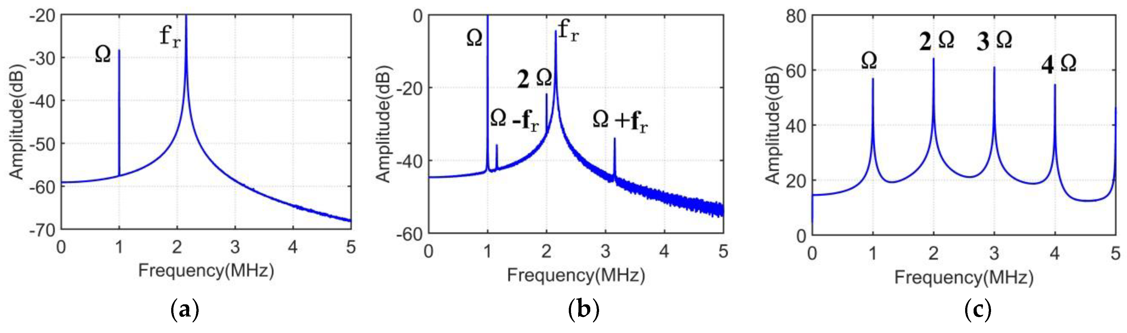
Thus, the solution of Equation (4) denotes the power spectrum of a Nd: YVO4 laser under frequency-shifted feedback. The results with different feedback levels using numerical solutions are shown in Figure 2. Three kinds of feedback levels are identified as weak, moderate, and strong feedback [42]. For the weak feedback level, there are two peaks at the relaxation oscillation frequency fr and shifted frequency Ω. When the feedback level is increasing, the signal to noise ratio (SNR) of the measuring light increases as well. However, the harmonic peaks (2Ω…) and parametric peaks (Ω+fr, Ω−fr …) appear. Especially, once the κ increases to the strong regime, the oscillating peak at fr disappears, and the signal at Ω and its harmonics (2Ω, 3Ω, 4Ω…) oscillate. In summary, the laser power spectrum with two peaks at the relaxation oscillation frequency fr and shifted frequency Ω is the desirable case for actual measurement. The appropriate κ can be adjusted by the ATT in the measurement. For strong feedback, the power spectrum is raised and disturbed by the shifted frequency signal, which cannot be utilized as a sensor.
The relative laser output power with the frequency of Ω is given as:
where ∆I denotes the intensity modulation of the measuring light, ϕs is a fixed phase, and ϕ is the phase related to the external cavity length. G is the frequency-dependent amplification factor, which can be expressed as:
The simulation based on the parameters of a Nd:YVO4 laser is as follows.
The nearer the shift frequency Ω is to the relaxation oscillation frequency fr, the larger the amplification factor G is, and it can be as high as 106 according to Figure 3. Therefore, the laser frequency-shifted optical feedback has ultrahigh sensitivity and excellent performance in the detection of weakly scattering light. However, it should be noted that the shift frequency Ω cannot coincide with the relaxation oscillation frequency fr in the actual experiment. Otherwise, the optical power spectrum will be in chaos, similar to that under a strong feedback level. Both the stability of the power spectrum and the signal amplification should be considered in the laser feedback interferometry.
2.2. Laser Confocal Feedback Tomography
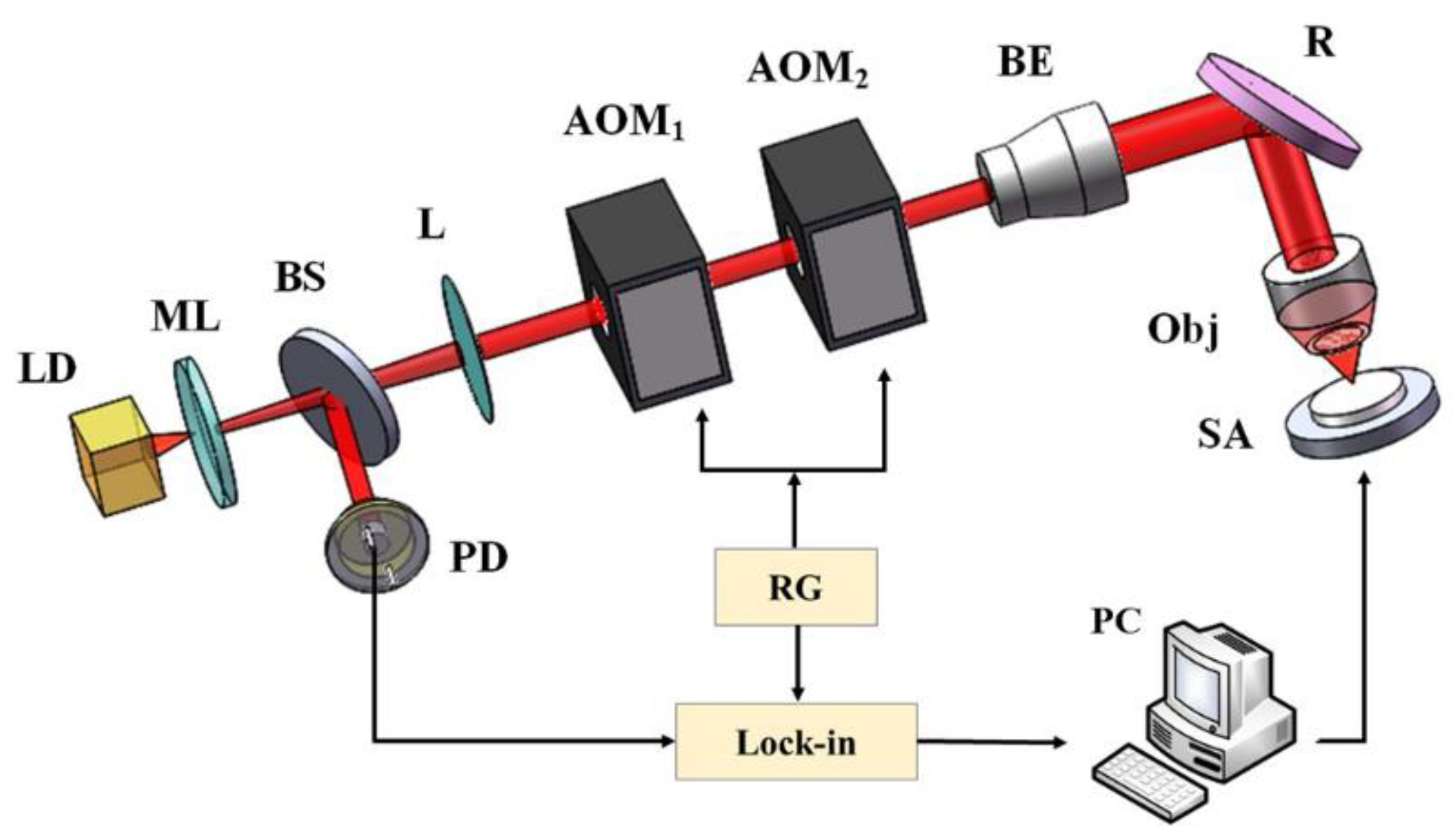
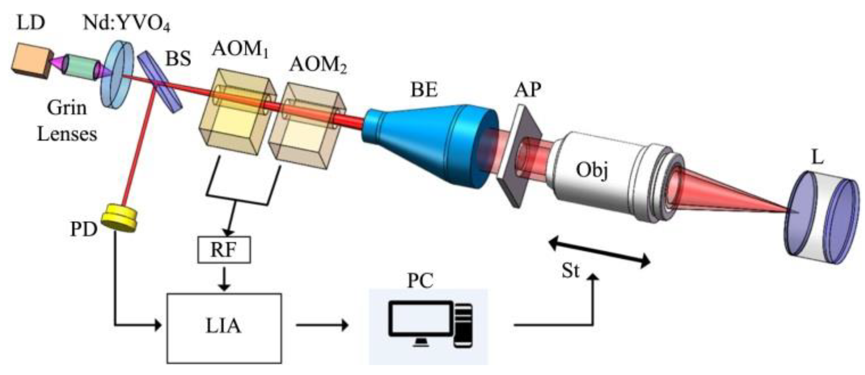
The basic schematic of the laser confocal feedback tomography is shown in Figure 4. The optical path before the AOMs is the same as that of the laser feedback interferometer as shown in Figure 1. Then the modulated light with the shift frequency of Ω/2 = |Ω1 − Ω2| is expanded by the beam expander (BE), reflected by the reflector (R), and finally, focused by the objective (Obj) onto the sample (SA). The reflected or scattered light by the SA returns back to the laser cavity along the same path, working as the measuring light with the shift frequency of Ω.
By sending the signal of the PD to the lock-in amplifier (Lock-in) as the measurement channel, generating the electrical signal with the Ω frequency from the radio-frequency generator (RG) as the reference channel, the intensity of the measuring light can be demodulated by the Lock-in. The optical power modulation of the measuring light can be induced as [38,39]:
I(u) is the light intensity response function of the traditional confocal system, and is given as [27,43]:
where u, ρ, and vd are the normalized de-focus parameter, radial coordinate, and diameter of the pinhole, respectively, and Kr is the normalized constant.
It is noted that there is no pinhole in Figure 4 because the laser in the setup is not only the light source but also the detector; therefore, the laser waist can be utilized as the pinhole filter. Thus, the structure of the laser confocal feedback tomography greatly simplified compared with the traditional confocal system.
3. Applications of the Laser Feedback Interferometer
3.1. Displacement Sensing
Displacement measurement is the basic application of the laser feedback interferometer. According to Equation (6), one cycle in the laser intensity modulation corresponds to half the wavelength in the length of the external cavity, which is similar to the traditional laser interferometer. Due to the existence of the amplification factor G, the laser feedback interferometer has a high sensitivity that it does not need a retroreflector or corner prism set on the target. Therefore, it is advantageous to realize the axial displacement measurement where no additional optical devices are installed.
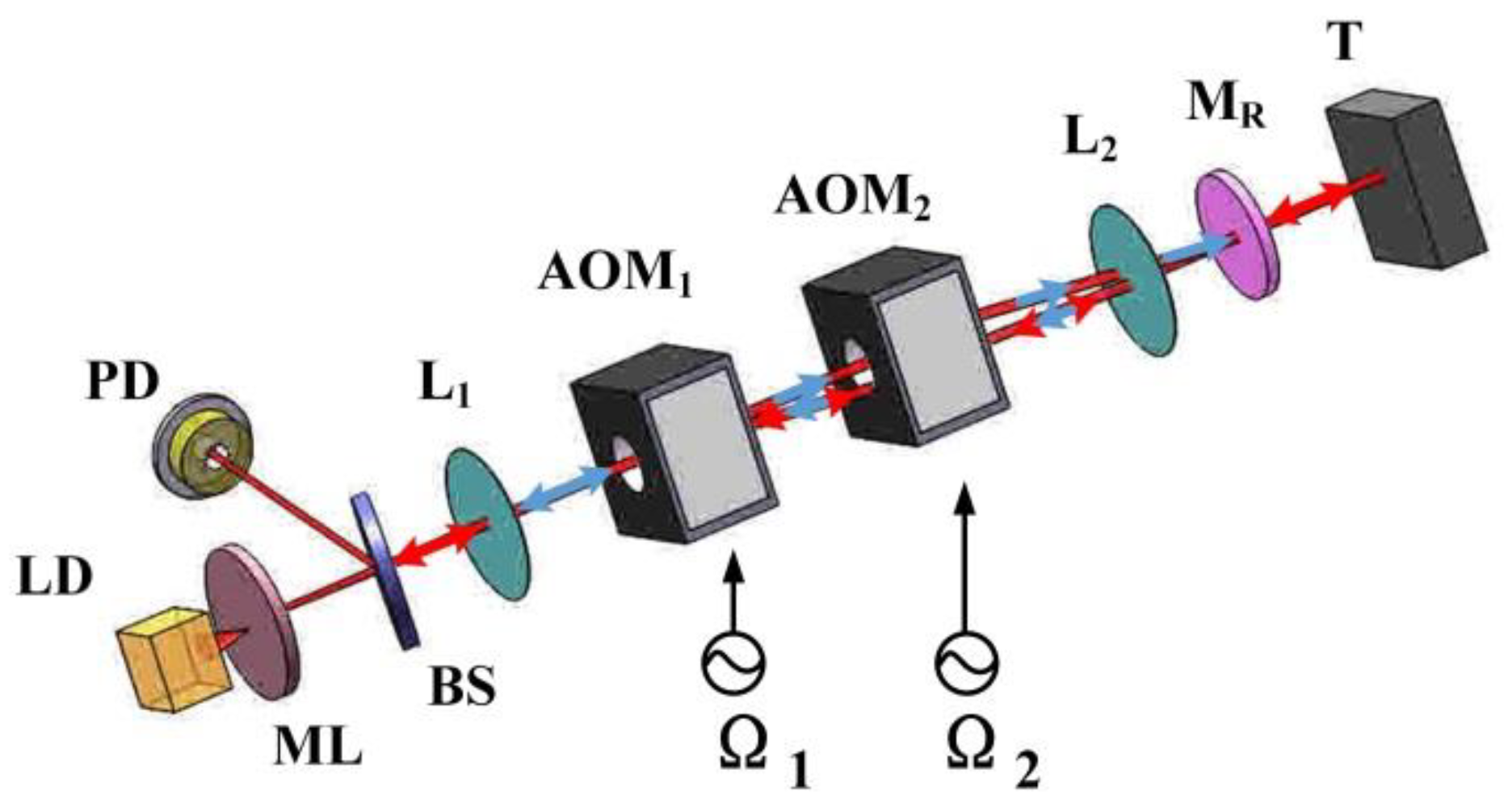
Wan [13] proposed a quasi-common-path configuration based on frequency shifting and multiplexing to compensate the air disturbance and the thermal effects of the components. The system structure is shown in Figure 5. It is innovative to put a reference mirror after the two AOMs to generate a feedback light. The original optical path without diffraction and the diffractive optical path with the shift frequency of Ω/2 = |Ω1 − Ω2| constitute a round-trip as the reference light, which is shown in blue arrows.
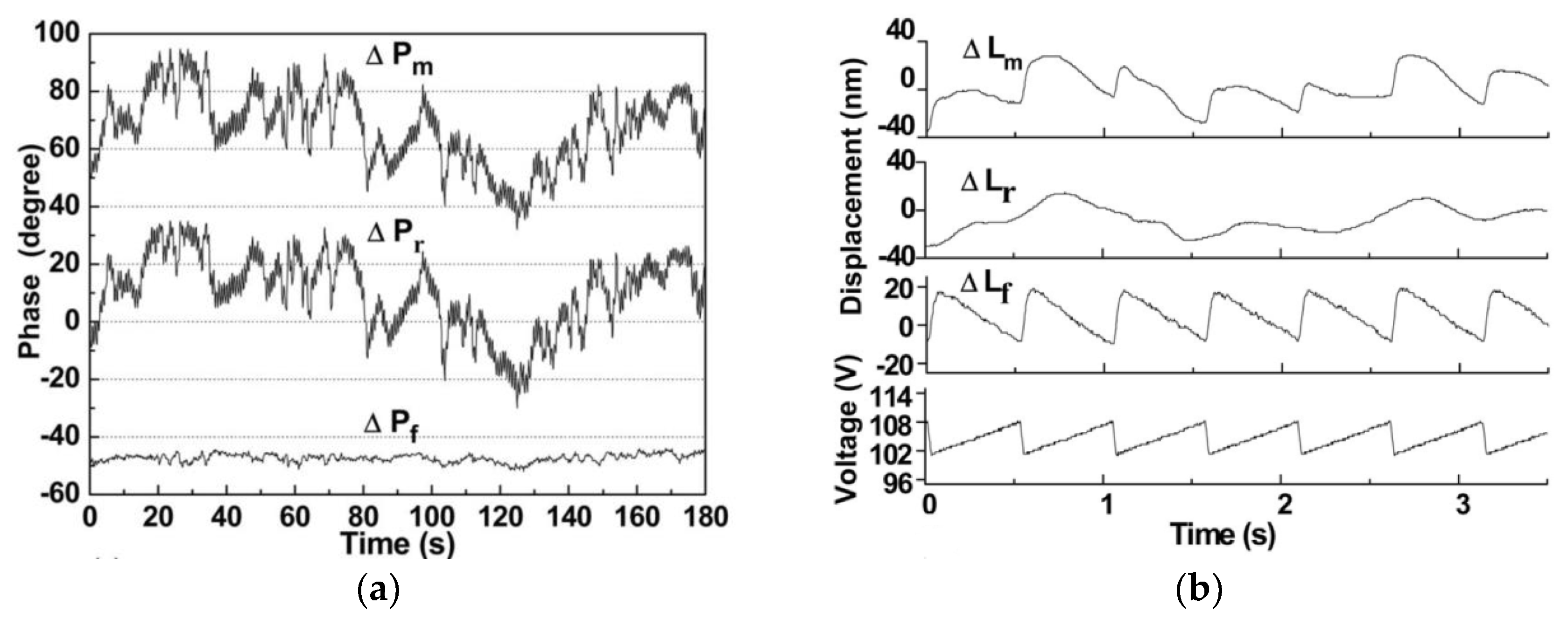
The displacement information of the measuring light and reference light can be demodulated at the frequency Ω/2 and Ω, respectively. The change of the displacement ΔL is related to the phase variation ΔP by:
where ΔPm is the phase variation of the measuring light, ΔPr is the phase variation of the reference light, ΔLm is the corresponding measurement displacement, ΔLr is the corresponding reference displacement, ΔPf is the final phase variation, and ΔLf is the final displacement.
The piezoelectric transducer (PZT) is tested in the system as the T in Figure 5. The reference mirror (MR) is placed 10 mm before the PZT. In the experiment, the PZT is driven by a ramp wave signal. The measured ΔPm and ΔPr, and the corresponding ΔLm, ΔLr, ΔPf, and ΔLf are shown in Figure 6. It is noted that the PZT vibration waveform cannot be revealed from ΔLm; however, it can be revealed from ΔLf accurately. The maximum nonlinear error of the ΔLf data is 1.8 nm, indicating that its short period resolution is better than 2 nm.
The quasi-common-path configuration has dramatically improved the performance of the laser feedback interferometer. However, two shortcomings remain to be improved. One is the measuring speed. The signal demodulation is based on the Lock-in in Ref. [13], which limits the measuring speed to be 100 μm/s. Zhang and Ren [44] proposed a new signal processing method replacing the Lock-in to a phase meter, and the measuring speed is improved to 10 mm/s. Then, Zhang [45] improved the performance of the system by replacing the laser source with a Nd: YVO4 crystal. The relaxation oscillation frequency increased from 300 kHz to 4.5 MHz, and the shifted frequencies were 2 MHz and 1 MHz, respectively. Finally, the measuring speed was improved to 120 mm/s.
The other shortcoming is the common path compensation. Due to the difference of the optical path between the measuring light and the reference light, the thermal effect produced by the AOMs is different; thus, quasi-common compensation cannot be completely eliminated. On the other hand, the position of the MR limits the compensation effect when sensing the displacement over a long distance. Ren [46] proposed a ring optical path configuration of the laser feedback interferometer. The paths of the reference light and the measured light coincide completely; thus, the thermal compensation effect is improved. Zhang [47,48,49] demonstrated a common-path heterodyne self-mixing interferometry with polarization and frequency multiplexing. The two mutual independent orthogonal polarized lights are used as the measuring and reference lights, of which the optical paths completely coincide in space; thus, the effect of the AOMs thermal creep and air disturbance can be eliminated. The short-term resolution is better than 2.5 nm, and the long-term zero drift is less than 60 nm over 7 h. Xu [50] proposed a novel approach to realize full path compensation laser feedback interferometry for remote sensing. The displacement of a steel block at a distance of 10 m is measured, of which the stability is ±12 nm over 100 s and ±50 nm over 1000 s, and the short-term resolution is better than 3 nm.
More recently, the two-dimensional (2-D) displacement measurement based on the self-mixing interferometry is revealed [14]. The system is shown in Figure 7. Two measuring beams at the different shift frequencies are incident on the same spot on the target. By heterodyne demodulating the phases of the two beams and deriving the relationship between the phases’ variations and the change of the in-plane and out-of-plane displacement, 2-D displacement measurement can be realized. Various movements in the track of Lissajous figures and random motion are measured in the experiments. The results show that the resolutions of the two dimensions are better than 5 nm and the standard deviation can be better than 0.1 μm.
The simultaneous measurements of in-plane and out-of-plane displacements are a significant issue to be researched, such as the grating interferometry [51,52], speckle pattern interferometry [53,54], digital image correlation [55,56], and laser Doppler distance sensing [57]. The resolution of the grating interferometer is a few nanometers, and the accuracy can reach a submicron scale. However, the 2-D grating needs to be set on the target, which limits the application. A laser Doppler distance sensor is appropriate for the dynamic position measurements of the fast-moving object, and the resolution of which is only on the submicron order. Speckle pattern interferometry and digital image correlation are two noncontact and full field displacement measurement methods, which are widely used in industrial nondestructive detection. However, they are limited to the static and quasi-dynamic displacement measurement field; the measurement range and accuracy are related to the speckle size obtained and come to a compromise in the application. Compared with other methods, laser feedback interferometry has the advantages of compactness, non-contact, high resolution, and high accuracy. However, the characteristic of the single-spot measurement limits the application in the full field measurement. It is a promising method to be applied in the 2-D deformation of materials measurement and 2-D thermal expansion measurement, among others.
3.2. Vibration Sensing
Besides the displacement sensing, the precise measurement of vibration has attracted wide attention as well. Vibration sensing can be utilized to analyze the dynamic characteristics of mechanical structures, fault diagnosis of mechanical systems, target identification, and sound visualization [58]. However, it is difficult to detect small vibration and displacement in many cases, especially the micro-vibration of non-cooperative targets at long distance.
Otsuka [16] proposed the real time nanometer vibration measurement using a self-mixing microchip solid-state laser. The experimental configuration is shown in Figure 8. The LiNdP4O12 (LNP) crystal with a 1-mm-thick plane-parallel Fabry–Perot cavity that is utilized as the microchip laser. The pump light is transformed into a circular beam using the anamorphic prism pairs and is focused onto the LNP crystal via an objective microscope lens. The output light is frequency-shifted by two AOMs and impinged upon a speaker with the Al-coated surface that is placed 90 cm from the laser. A frequency demodulation circuit, a digital oscilloscope, and a radio-frequency spectrum analyzer are utilized in the signal processing.
Figure 9a shows the power spectra for several voltages applied to the speaker. The measured vibration amplitudes (Av,m) at the modulation frequency of 8.42 kHz with the carrier frequency of 500 kHz are plotted in Figure 9b. The linear relation was Av,m/Va = 59 nm/V for the speaker we used. The measurable minimum vibration amplitude was 1 nm according to the carrier-to-noise ratio in the absence of a voltage to the speaker. The velocity range in the present vibrometry was 1 μm/s to 10 cm/s in the vibration frequency range 20 Hz to 20 kHz. The temporal evolutions of nanometer vibrations were measured by analyzing modulated output waveform using the Hilbert transformation. The almost unheard sound of music below a 20-dB pressure level is reproduced by the system.
Furthermore, three-channel real time nanometer vibration [59] was successfully developed with three pairs of acoustic optical modulators and a three-channel frequency-modulated wave demodulation circuit, realizing simultaneous independent measurement of three different nanometer-vibrating targets. On the other hand, the vibration of targets placed 2.5 km away through single-mode optical fiber access was successfully measured [60], due to the effective long-haul self-mixing interference.
There are also other researchers applying self-mixing interference effects in the vibration sensing. Huang [61] proposed a vibration system extreme points model and self-mixing vibration sensor based on the effect of LD; the amplitude-frequency response curve of the loudspeaker is drawn, and the value of the piezoelectric coefficient of PZT was obtained. Tao [62] presented a signal-processing synthesizing wavelet transform, and a Hilbert transform employed to the micro-vibration measurement based on the semiconductor laser self-mixing technology. The real-time micro vibration with a nanometer resolution and a much wider bandwidth than conventional modulation methods were proved. Dai [63] proposed the self-mixing interferometry in a fiber ring laser and its application for vibration measurement. The maximum error of the amplitude was about λ/10, and the maximum relative error of the frequency was about 10%.
3.3. Particle Sensing
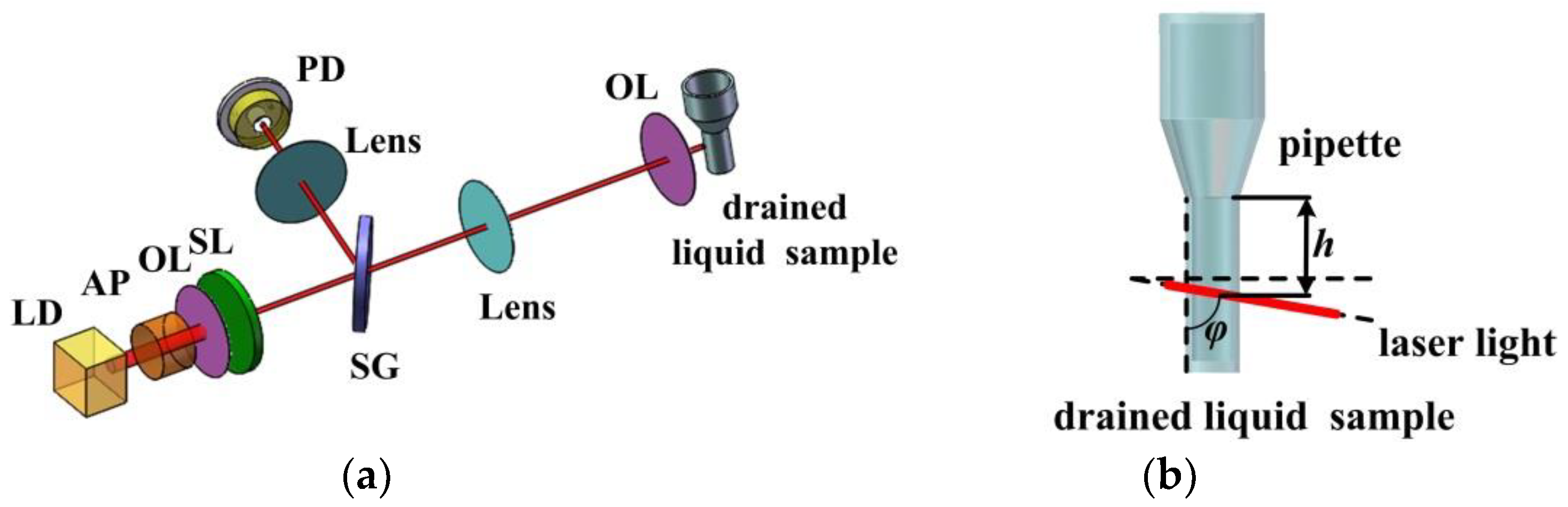
The self-mixing laser Doppler velocimeter is one of the promising technologies applied in the observation and detection of the particles flowing in liquid [64,65], which has been recognized as the simplest, most cost-effective, and most self-aligned metrology. The system is shown in Figure 10 using a drained suspension including polystyrene latex standard spheres (PLS). The output power is modulated by the frequency-shifted scattered light generated by the motion of moving targets. When the moving target moves at a uniform velocity, the Gaussian power spectrum can be observed, and the peak frequency corresponds to the Doppler shift frequency fd.
The angle of the incident laser light is set at ψ = 16° to the surface of the drained suspension. Here it is noted that the Gaussian spectrum is marked by the noise if the intensity of the light scattered from the moving particles is very weak. In this case, the motion can be revealed in its higher harmonics when the frequency of the relaxation oscillation of the laser output, fo2, is made to coincide with fd by tuning the pump current of the laser (ic) at ic = 335 mA, as shown in Figure 11b,c. Thus, the ultrahigh sensitivity measurement of extremely weak scattered light can be achieved. The spectral peak G in Figure 11 reflects the motion of the particles passing through the incident laser light. The frequency of the Gaussian is fd = 500 kHz, which is related to the average velocity of the particles. The amplitude is associated with the intensity of the light scattered, which is proportional to the concentration of the particles.
3.4. Liquid Evaporation Rate Measurement
Liquid evaporation measurement is fundamental in many industrial applications and scientific research, such as quantitative analysis, and physical and chemical reaction process monitoring. The common methods used to measure the liquid level variation, including the capacitive sensors, the fiber liquid level sensor, the laser triangulation, etc., are contact-based or have limited accuracy. Tan [66] reported the application of real-time evaporation of the liquid measurement based on the laser feedback interferometer. The experimental system is shown in Figure 12. The structure of the instrument belongs to the quasi-common-path laser feedback interferometer [44]. A hollow arm with a right-angled prism fixed on the edge is installed at the interface of the interferometer, turning the laser beam 90 degrees and adjusting it incident perpendicularly onto the liquid surface. Four different transparent liquids, including distilled water, absolute alcohol, acetone, and ether, are measured in the system. The results show that real-time direct measurement of liquid evaporation and liquid level measurement with a nanometer order is realized.
3.5. Refractive Index Measurement
The refractive index n of a material is a physical quantity that describes how light propagates through the material. Thus, accurate measurement of material refractive index is significant for optical system design. Different methods have been developed. The minimum deviation method has the highest accuracy (10−6), but the sample needs to be prism-shaped, which is complicated and costly. An Abbe refractometer is the most commonly used instrument, but the measurement range is limited from 1.3 to 1.7, and the accuracy is 10−4. In comparison, the interferometry methods have many advantages, such as easy sample processing, low cost, wide measuring range, high measurement accuracy, and they have been widely researched in the refractive index measurement field, including Michelson interferometry [67], Mach–Zehnder interferometry [68], Fabry–Perot interferometry [69] and plasmonic interferometry [70,71], etc. The common principle of these interferometry methods is to measure the optical path change caused by the sample rotation or displacement. However, these interferometers cannot avoid the environmental disturbance, and the measurement accuracies are hard to be further improved. Xu [72,73] proposed a method to measure the refractive index and thickness simultaneously based on the laser feedback interferometry. Compared with other methods, the influence of environmental disturbance can be eliminated by the quasi-common path structure of the laser feedback interferometry, and the absolute uncertainty in the refractive index measurement reaches ≈10−5. On the other hand, the refractive index measurement range is larger than the conventional interferometry due to the high sensitivity of the system. The system is shown in Figure 13.
By rotating a transparent parallel sample inside the external feedback cavity, the optical path difference ΔL can be derived as:
where λ is the laser wavelength; d is the thickness of the sample; n is the refractive index to be measured; n0 is the refractive index of the air; θ0 and θ are the angles between the laser beam and the normal of sample surface before and after rotation, respectively; and Pm and Pr are the phase variations of the measurement light and the reference light, respectively, which are demodulated by the phase meter.
θ and ΔL are measured at multiple angles in the experiment, then the overdetermined equation can be solved, and the refractive index of the sample can be obtained together with the thickness of the sample. Due to the high sensitivity of the laser feedback interferometry, the method can be used to measure the low transmittance materials, including calcium fluoride (CaF2), fused silica, and zinc selenide (ZnSe). The refractive indexes cover a large range from 1.42847 to 2.48272. The results demonstrate that the system has absolute uncertainties in the refractive index measurement of ≈10−5.
Xu [74] also reported a novel method to measure the liquid refractive index based on the double-beam laser frequency-shift feedback. The system is shown in Figure 14. Two parallel beams are adjusted to each monitor the displacement of the liquid surface and the MR at the bottom of the tank. When the liquid level increases by Δh, the change of the two external cavity lengths are:
where n0 is the air refractive index, and n is the liquid refractive index to be measured, which can be expressed as:
Since the liquid refractive index depends entirely on the displacement measurement of the two beams, the refractive index measurement is also traceable. Thus, the results can be used as a reference for calibration of the liquid refractive index. Five different liquid samples, including the distilled water, ethanol, cyclohexane, silicone oil, engine oil, and NaCl solution with various concentrations, are measured in the experiment, which proves that the repeatability is better than 0.00005.
3.6. Thermal Expansion Coefficient Measurement
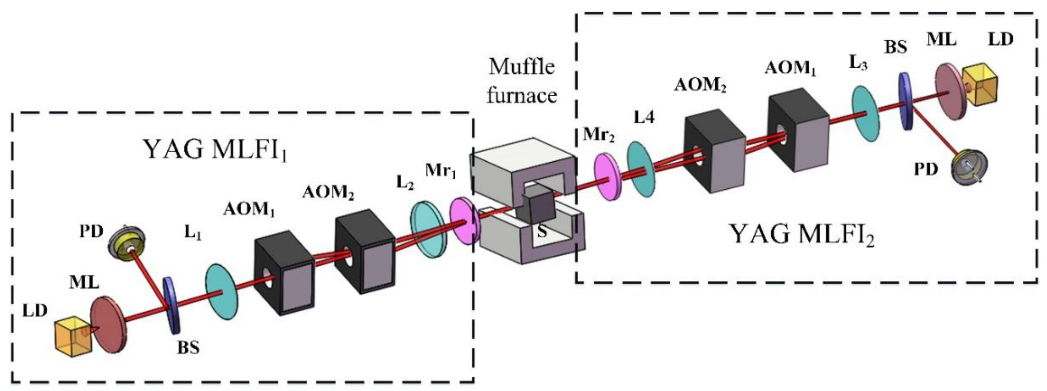
The thermal expansion coefficient is one of the most fundamental quantities of materials, which describes how the size of an object changes due to the temperature variation. The precise measurement of the thermal expansion coefficient is significant in basic scientific research and industrial application. Zheng [75,76] proposed a non-contact method to measure the thermal expansion coefficient of materials utilizing a pair of Nd: YAG microchip laser feedback interferometers (MLFIs). The schematic diagram of the system is shown in Figure 15.
The sample with a supporter is placed in the middle of the furnace chamber. Two symmetric laser feedback interferometers output two measurement beams, which are incident on each surface of the sample perpendicularly and coaxially, to compensate for the influence of the sample supporter distortion. Two Mrs are set close to the muffle furnace, generating the two reference signals, revealing the air flow and thermal lens effect disturbances outside the furnace chamber. By subtracting it, S1m − S1r and S2m − S2r are the compensated displacement of the two laser feedback interferometers, respectively. Thus, the length change of the sample from T0 to T1 can be expressed approximately as:
where S1m and S2m are the displacements of the two measurement beams, and S1r and S2r are the displacements of the two reference beams. Then, the thermal expansion coefficient can be obtained as:
where L0 is the length of the sample at T0.
The aluminum and the steel 45 samples are measured in the experiment from room temperature to 748 K, which proves that the measurement repeatability of thermal expansion coefficient is better than 0.6 × 10⁻⁶ (K−1) in the range 298 K–598 K and the high-sensitive non-contact measurement of the low reflectivity surface induced by the oxidization of the samples in the range of 598 K–748 K.
The existing methods for the thermal expansion coefficient measurement mainly include a mechanical dilatometer [77], speckle pattern interferometry [78], Fabry–Perot interferometry [79], etc. The mechanical dilatometer is an old and frequently utilized method, which has a wide temperature range but cannot satisfy the requirement for high-precision measurement. The performance of speckle pattern interferometry mostly depends on the algorithm model and speckle size; the measurement range and accuracy usually come to a compromise. Optical interference has a great performance in resolution and precision, but the measurable materials and working temperature range are limited. The thermal expansion coefficient measurement performed at the high temperature in our system solves the issues in special applications, such as aerospace materials, where the temperature of the environment can be as high as thousands of degrees, and the parameter of materials needs to be calibrated. It also shows the excellent advantages of the setup, because many measurement methods cannot be utilized at such high temperatures.
3.7. Gear Measurement
The possibility of the gear measurement using the laser feedback interferometer is discussed here. The gear is placed on a rotation stage with the measuring light incident perpendicularly at a certain eccentricity distance as shown in Figure 16. The unidirectional linear displacement curve is obtained in the experiment when the gear rotates in one direction. According to the Doppler theory, the integral of the velocity along the axis of light is the measuring displacement, which can be deduced as d = H × θ. Thus, the displacement measurement is related to the eccentricity distance and the rotation angles. The result is in agreement with the derived formula with the parameters of θ = 25° and H = 20 mm. Therefore, the system can be utilized for the measurement of gear speed or the alignment error of the central gear shaft. In further research, the gear profile measurement is considered and hopefully to be realized in on-line monitoring.
4. Applications of the Laser Confocal Feedback Tomography
4.1. Microstructure Imaging and Measuring
The schematic diagram of the laser confocal feedback tomography is shown in Figure 4 above. To realize the three-dimensional scanning in the inner structure of the sample, we fix the objective lens in a vertical translation stage to scan in the longitudinal direction, while the sample is set in the two-dimensional translation stage to get the horizontal movement.
The theoretical lateral resolution of the system is approximately given by Δx = 0.61λ/(√2×NA), for the objective with the NA = 0.42 utilized in the experiment, corresponding to 1.1 μm. The vertical resolution is evaluated via scanning the defocus curve and measuring the full width at half maximum (FWHM), which is about 15–20 μm. The system can be applied in the imaging of the structure of the micro-electro-mechanical system [80,81]. For example, the sandwich type sample with the patterned layer etched in a silicon film of 1 mm and two pieces of 0.5 mm thick glass is measured. The 2-D cross-sectional imaging with the depth of 3 mm and lateral range of 6 mm is obtained as shown in Figure 17.
A biological sample, such as onion inside water, can also be measured using the laser confocal feedback tomography [39]. Two onion samples are adopted, one (named onion-1) containing a pin that is inserted 0.5 mm beneath its surface, and the other (named onion-2) containing two separated pins inserted 1 mm below its surface. The section of the pin’s tip immerged into the onion is selected to obtain its 2-D cross-sectional image in the X-Y plane. As illustrated in Figure 18, the cross-sectional images denoted by the double-dot-dash lines clearly indicate the profile of the pins’ tip. What is more, the position of the pins in the onions can also be confirmed.
Furthermore, Wang [82] improved the axial resolution to nanometers when measuring the microstructure inside the sample based on the laser confocal feedback tomography by using the linear region EF in the defocusing curve as shown in Figure 19. It should be noted that the linear region EF needs to be calibrated experimentally. First, the light is focused on the sample surface; then the objective is moved at a certain step in the longitudinal direction using a one-dimensional motorized scanning stage with the resolution of 0.5 nm, and simultaneously detects the amplitude A. The fitted line is obtained between the amplitude and the defocus distance. With the different objective lenses utilized in the system, different linear ranges and different axial resolutions are realized. The experimental measurement axial resolutions are 2, 5, and 11 nm with the objective NA values of 0.65, 0.55, and 0.3, respectively.
When measuring the samples, the light is focused on the interesting point first, and then the sample is scanned in the horizontal direction. During the scanning, the amplitude of the feedback light intensity varies with the structure variation. The amplitude variation can be converted to the distance according to the calibrated line. Thus, the structure of the sample is measured at last. A micro-gyroscope is measured as shown in Figure 20. The system can realize the noninvasive inner structure measurement through the protection glass. The tilt angle of the inner side of the rotor should be tested according to actual demands. According to the vertical and horizontal structure variations of the rotor edge, tan(θ) can be calculated, and then θ can be obtained to estimate the verticality of the rotor edge. The results are in agreement with the value measured by the destructive method.
It can be deduced that the laser optical feedback imaging is well-adapted for various fields and has been widely researched. Bertling [83] introduced the optical feedback interferometry for the two-dimensional visualization of acoustic fields. Several pressure distributions including progressive waves, standing waves, diffraction, and interference patterns are presented. Girardeau [84] applied the laser optical feedback imaging setup to the detection of ultrasound vibrations with nanometric amplitude. The transient-harmonics ultrasound vibrations propagating in water were detected at the air/water interface, which shows the potential for the detection of photoacoustic signals. Mowla [85] proposed a compact system using a semiconductor laser as both transmitter and receiver. Three phantoms containing macro-structural changes in optical properties were imaged, which revealed the discrimination ability between healthy tissue and a tumor. Hugon [86] proposed a galvanometric mirrors scanner moving the beam on the sample and optimized the scanner positioning to reduce the vignetting effects. A micro-structured silicon sample and a red blood cell were presented.
4.2. Profilometry
In Section 4.1, only the amplitude information of the light is demodulated and utilized. When the system is applied to a surface measurement, the phase information can be demodulated, together with the amplitude information, to reveal the micro-nano structure [38,87]. The system is shown in Figure 21. Both the intensity modulations Im(2Ω) and Ir(Ω) can be obtained from the PD. By demodulating Im(2Ω), not only the amplitude (A), but also the phase (Pm) can be obtained. At the same time, the phase information (Pr) from Ir(Ω) is used to compensate the Pm to achieve high accuracy in phase measurement, and thereby result in the high axial accuracy with nanometer resolution.
When the profilometry is conducted, the objective lens is scanned in the longitudinal direction to obtain the defocus response curve, locating the sample surface. After that, scanning the sample in the horizontal direction and simultaneously detecting the feedback light intensity. When measuring the height difference Δh of two lateral positions on the sample surface, it obtains the integral number n of λ/2 contained in Δh based on the amplitude (A) variation of the laser intensity with the range of 10 μm, and the fractional number s of λ/2 using the phase measurement with a resolution of ≈2 nm. Finally, the height difference is computed as:
where ζ is a calibrated coefficient to take into consideration the influence of the high NA of the objective, whose value is carefully calibrated to be 0.93.
4.3. Lens Thickness Measurement
Lens thickness measurements play an important role in the optical industry and optical systems. Various optical methods have been applied in the lens thickness noncontact measurement. A machine vision method [88] has advantages of continuous measurement, it is flexible in the production line, and the accuracy is less than 0.005 mm. Chromatic confocal sensors [89] are based on spectrally broadband light to realize a special optical probe. The measuring range and the accuracy are influenced by the designed probe and the dispersion of the measured object material. Low coherence interferometry [90] is utilized to measure the central thickness of soft and rigid contact lenses with the accuracy of a few micrometers. A laser differential confocal technique [91,92] realizes the high-precision measurement of the lens’ axial space by detecting the absolute zero of an axial intensity curve. The measurement uncertainty is less than 0.05% for the thickness. Considering the high sensitivity of the laser feedback effect, it has great potential for the axial positioning, especially the multilayer lenses or the coated lens with the high anti-reflecting film. Tan [93] proposed a new method to realize the lens thickness and air gap measurement, as shown in Figure 22. The annular pupil is inserted into the path before the objective lens to create the annular beam, in order to reduce the axial aberration and decrease the positioning error.
When the objective lens moves along the optical axis, and the focused beam passes through the surfaces of the lenses, the defocus response curve can be obtained at each interface. The peak of the curve corresponds exactly to the beam focusing on the surface of the lens, as shown in Figure 23. Thus, the axial positioning can be realized via the synchronous acquisition of the light intensity and the displacement of the stage. Considering the refraction and reflection when the light passes through the lens, the relationship between the lens thickness and the axial positioning displacement can be deduced as:
where ε is the ratio of the inner and outer diameter of the AP, Ti is the ray tracing process function related to the lenses measured, and di is the displacement between each interface.
Different materials and kinds of lenses are measured in the experiment, including K9 plain glasses, fused silica plain glass, and K9 biconvex lens. The results prove that the uncertainty of the axial positioning is better than 0.0005 mm and the accuracy reaches the micron range.
4.4. Laser Confocal Feedback Imaging Combined with Other Technologies
4.4.1. Depth of Focus Extension in Laser Frequency-Shifted Feedback Imaging
For optical imaging, there is always a trade-off between the depth of focus (DOF) and the resolution [94,95]. Therefore, extending the DOF has drawn much attention, and various methods have been put forward. Numerically reconstructing a higher-resolved picture from a traditional beam is a main category of the methods, which is challenged by the decline of ballistic photons with the longer DOF. The laser feedback effect has the high sensitivity and could solve the problem. Thus, Lu [96] reported the depth of focus extension in laser frequency-shifted feedback imaging by filtering in the frequency domain. The system is shown in Figure 24. The measuring beam with the frequency shift after passing the BE is reflected by two galvanometric mirrors, then converged by objective lens L5; however, with the target located at the defocus plane.
The original image is acquired via a 2-D scanning point by point, which can be described as the convolution of the point diffusion function (PSF) with the target plane. In theory, the Fourier transform of PSF (CTF) at a defocus length (DL) of L can be deduced as:
By filtering in the frequency domain, the new CTF can be obtained as:
The inverse Fourier transform of the CTF corresponding to the new PSF can be calculated using:
Therefore, a resolution of r0/√2 is obtained by filtering in the frequency domain, and it is possible to keep the resolution even in the far defocus plane.
A three-dimensional target with three steps is tested in the experiment, and the processing of gradual refocusing is demonstrated as shown in Figure 25. The original blurred image is obtained using a 2-D scan. By filtering the image matrix in the frequency domain with a sequence of DL = 0.1:0.1:100 mm, three clear images of different steps can be obtained. The difference between the values of DL in filtering is exactly 5 mm, which equals the step height. In this way, the information along the optical axis can be obtained. The numerical experiments reveal that its depth of focus is capable of being extended to four times the length of the objective focal length.
4.4.2. Ultrasound Modulated Laser Confocal Feedback Imaging
When imaging objects inside turbid media, the number of ballistic photons decreases rapidly, compared to the scattered photons, as the penetration depth increases. As a result, the SNR is greatly reduced. The quality of the laser confocal feedback imaging is also affected by the scattered photons [39], and the generated speckles reduce the image contrast as well as the SNR. To solve the problem, Zhu [97] applied the ultrasound-modulated technology in the laser confocal feedback imaging. The system is shown in Figure 26. Except for the optical path focused into the sample, the ultrasound transducer is utilized, and the ultrasonic wave is focused into the same spot as well. As a result, the photons in the focal region are modulated with the shift frequency of the ultrasonic driving frequency [98,99]. Thus, the interesting photons are distinguished from the other scattered photons as the noise photons fall outside the focal region in the frequency domain. This is promising for reaching a larger penetration depth as well as a better SNR due to the reduction of noise photons.
When the measuring light returns to the laser cavity, the optical power modulation can be deduced as:
where ΔI denotes the intensity modulation of the measuring light, Is is the output power of the solitary laser, M1 is the ultrasound one-sided modulation depth, I(u) is the light intensity of the confocal system, κ is the coefficient of the feedback light strength, G is the frequency dependent amplification factor, ϕs is a fixed phase, and ϕ is the phase related to the external cavity length.
The simulations and experiment are conducted in the paper. The contrasting experimental results with the traditional laser confocal feedback imaging are shown in Figure 27, proving that it is an effective method to realize a better SNR with the increasing of the scattering coefficient and focused depth. Compared with other optical methods, it is possible to reach both a larger imaging depth and a better SNR, especially in the turbid media.
5. Conclusions
In this paper, an overview of the laser feedback technology is presented. Two major configurations, the laser feedback interferometer and the laser confocal feedback tomography, are introduced theoretically, and a series of applications are described respectively.
The laser feedback interferometer has great potential because it does not need a retroreflector or corner prism set on the target. However, the stability and the performance indicators of the instrument are not as good as the He-Ne laser interferometer nowadays. Therefore, improving the performance of the laser feedback interferometer to be comparable with the traditional laser interferometer is a major research area, which includes speed improvement [44,45] and common path compensation [46,47,48]. On the other hand, research on the application is an important part to solve the scientific or industrial problem utilizing the ultra-high sensitivity, such as the measurement of refractive index, thermal expansion coefficient, liquid evaporation rate, etc. [66,72,73,74,75,76].
The laser confocal feedback tomography is proposed to reach a greater imaging depth compared with the confocal microscopy or optical coherence tomography [38,39]. It also shows great performance in the structure measurement of the micro-electro-mechanical system [80,81,82]. However, the system is also challenged to realize both high resolution and large penetration depth the same as the other optical methods. Therefore, combining other technologies with the advantages of the laser confocal feedback tomography is interesting research, such as the numerically reconstructing imaging to extend the DOF and ultrasound-modulated technology to improve the SNR [96,97].
In conclusion, the frequency-shifted optical feedback can be applied in a vast range of fields such as metrology, physical quantities measurement, imaging, microstructure measurement, and others. It is promising to be developed in further study, and in new fields combined with other technologies in future research.
Author Contributions
K.Z. initiated the manuscript. All authors participated in the revision of the manuscript. Y.T. provided overall supervision.
Funding
This research was funded by the National Science Fund for Excellent Young Scholars of China, grant number 51722506; the National Natural Science Foundation of China, grant number 61475082; and the National Natural Science Foundation of China, grant number 61775118.
Conflicts of Interest
The authors declare no conflict of interest.
References
- King, P.G.R.; Steward, G.J. Metrology with an optical maser. New Sci. 1963, 17, 14. [Google Scholar]
- Taimre, T.; Nikolić, M.; Bertling, K.; Lim, Y.L.; Bosch, T.; Rakić, A.D. Laser feedback interferometry: A tutorial on the self-mixing effect for coherent sensing. Adv. Opt. Photonics 2015, 7, 570–631. [Google Scholar] [CrossRef]
- Li, J.; Niu, H.; Niu, Y. Laser feedback interferometry and applications: A review. Opt. Eng. 2017, 56, 050901. [Google Scholar] [CrossRef]
- Otsuka, K.; Kawai, R.; Asakawa, Y. Ultrahigh-sensitivity self-mixing laser Doppler velocimetry with laser-diode-pumped microchip LiNdP4O12 lasers. IEEE Photonics Technol. Lett. 1999, 11, 706–708. [Google Scholar] [CrossRef]
- Timmermans, C.J.; Schellekens, P.H.J.; Schram, D.C. A phase quadrature feedback interferometer using a two-mode He-Ne laser. J. Phys. E Sci. Instrum. 1978, 11, 1023. [Google Scholar] [CrossRef]
- Besnard, P.; Jia, X.; Dalgliesh, R.; May, A.D.; Stephan, G. Polarization switching in a microchip Nd: YAG laser using polarized feedback. J. Opt. Soc. Am. B 1993, 10, 1605–1609. [Google Scholar] [CrossRef]
- Lang, R.; Kobayashi, K. External optical feedback effects on semiconductor injection laser properties. IEEE J. Quantum Electron. 1980, 16, 347–355. [Google Scholar] [CrossRef]
- Lenstra, D.; Van Vaalen, M.; Jaskorzyńska, B. On the theory of a single-mode laser with weak optical feedback. Phys. B+C 1984, 125, 255–264. [Google Scholar] [CrossRef]
- Wang, W.M.; Boyle, W.J.O.; Grattan, K.T.V.; Palmer, A.W. Self-mixing interference in a diode laser: Experimental observations and theoretical analysis. Appl. Opt. 1993, 32, 1551–1558. [Google Scholar] [CrossRef]
- Bosch, T.; Servagent, N.; Lescure, M. A displacement sensor for spectrum analysis using the optical feedback in a single-mode laser diode. Proc. IEEE Instrum. Meas. Technol. Conf. 1997, 2, 870–873. [Google Scholar] [CrossRef]
- Otsuka, K. Effects of external perturbations on LiNdP4O12 lasers. IEEE J. Quantum Electron. 1979, 15, 655–663. [Google Scholar] [CrossRef]
- Arecchi, F.T.; Lippi, G.L.; Puccioni, G.P.; Tredicce, J.R. Deterministic chaos in laser with injected signal. Opt. Commun. 1984, 51, 308–314. [Google Scholar] [CrossRef]
- Wan, X.; Li, D.; Zhang, S. Quasi-common-path laser feedback interferometry based on frequency shifting and multiplexing. Opt. Lett. 2007, 32, 367–369. [Google Scholar] [CrossRef] [PubMed]
- Zhu, K.; Guo, B.; Lu, Y.; Zhang, S.; Tan, Y. Single-spot two-dimensional displacement measurement based on self-mixing interferometry. Optica 2017, 4, 729–735. [Google Scholar] [CrossRef]
- Otsuka, K. Self-mixing thin-slice solid-state laser Doppler velocimetry with much less than one feedback photon per Doppler cycle. Opt. Lett. 2015, 40, 4603–4606. [Google Scholar] [CrossRef]
- Otsuka, K.; Abe, K.; Ko, J.Y.; Lim, T.S. Real-time nanometer-vibration measurement with a self-mixing microchip solid-state laser. Opt. Lett. 2002, 27, 1339–1341. [Google Scholar] [CrossRef] [PubMed]
- Abe, K.; Otsuka, K.; Ko, J.Y. Self-mixing laser Doppler vibrometry with high optical sensitivity: Application to real-time sound reproduction. New J. Phys. 2003, 5, 8. [Google Scholar] [CrossRef]
- Sudo, S.; Miyasaka, Y.; Nemoto, K.; Kamikariya, K.; Otsuka, K. Detection of small particles in fluid flow using a self-mixing laser. Opt. Express 2007, 15, 8135–8145. [Google Scholar] [CrossRef]
- Zhang, S.; Tan, Y.; Zhang, S. Non-contact angle measurement based on parallel multiplex laser feedback interferometry. Chin. Phys. B 2014, 23, 114202. [Google Scholar] [CrossRef]
- Szwaj, C.; Lacot, E.; Hugon, O. Large linewidth-enhancement factor in a microchip laser. Phys. Rev. A 2004, 70, 033809. [Google Scholar] [CrossRef]
- Zhang, S.; Sun, L.; Tan, Y. Spectrum broadening in optical frequency-shifted feedback of microchip laser. IEEE Photonics Technol. Lett. 2016, 28, 1593–1596. [Google Scholar] [CrossRef]
- Qin, C.; Feng, J.; Zhu, S.; Ma, X.; Zhong, J.; Wu, P.; Jin, Z.; Tian, J. Recent advances in bioluminescence tomography: Methodology and system as well as application. Laser Photonics Rev. 2014, 8, 94–114. [Google Scholar] [CrossRef]
- Liba, O.; Lew, M.D.; SoRelle, E.D.; Dutta, R.; Sen, D.; Moshfeghi, D.M.; Chu, S.; de La Zerda, A. Speckle-modulating optical coherence tomography in living mice and humans. Nat. Commun. 2017, 8, 15845. [Google Scholar] [CrossRef] [PubMed] [Green Version]
- Hillman, E.M.; Burgess, S.A. Sub-millimeter resolution 3D optical imaging of living tissue using laminar optical tomography. Laser Photonics Rev. 2009, 3, 159–179. [Google Scholar] [CrossRef] [PubMed] [Green Version]
- Bychkov, A.; Simonova, V.; Zarubin, V.; Cherepetskaya, E.; Karabutov, A. The Progress in Photoacoustic and Laser Ultrasonic Tomographic Imaging for Biomedicine and Industry: A Review. Appl. Sci. 2018, 8, 1931. [Google Scholar] [CrossRef]
- Wang, L.V.; Wu, H. Biomedical Optics: Principles and Imaging; John Wiley & Sons: Hoboken, NJ, USA, 2007; pp. 1–8. ISBN 978–0-471-74304-0. [Google Scholar]
- Wilson, T. Confocal Microscopy; Academic Press: London, UK, 1990; pp. 1–64. ISBN 978–1-4899-1494-1. [Google Scholar]
- Qiu, L.; Liu, D.; Zhao, W.; Cui, H.; Sheng, Z. Real-time laser differential confocal microscopy without sample reflectivity effects. Opt. Express 2014, 22, 21626–21640. [Google Scholar] [CrossRef] [PubMed]
- Wang, Y.; Qiu, L.; Zhao, X.; Zhao, W. Divided-aperture differential confocal fast-imaging microscopy. Meas. Sci. Technol. 2017, 28, 035401. [Google Scholar] [CrossRef]
- Durduran, T.; Choe, R.; Baker, W.B.; Yodh, A.G. Diffuse optics for tissue monitoring and tomography. Rep. Prog. Phys. 2010, 73, 076701. [Google Scholar] [CrossRef] [Green Version]
- Eggebrecht, A.T.; Ferradal, S.L.; Robichaux-Viehoever, A.; Hassanpour, M.S.; Dehghani, H.; Snyder, A.Z.; Hershey, T.; Culver, J.P. Mapping distributed brain function and networks with diffuse optical tomography. Nat. Photonics 2014, 8, 448–454. [Google Scholar] [CrossRef] [Green Version]
- Hong, G.; Antaris, A.L.; Dai, H. Near-infrared fluorophores for biomedical imaging. Nat. Biomed. Eng. 2017, 1, 0010. [Google Scholar] [CrossRef]
- Sevick-Muraca, E.M. Translation of near-infrared fluorescence imaging technologies: Emerging clinical applications. Annu. Rev. Med. 2012, 217–231. [Google Scholar] [CrossRef] [PubMed]
- Huang, D.; Swanson, E.A.; Lin, C.P.; Schuman, J.S.; Stinson, W.G.; Chang, W.; Hee, M.R.; Flotte, T.; Gregory, K.; Puliafito, C.A. Optical coherence tomography. Science 1991, 254, 1178–1181. [Google Scholar] [CrossRef] [PubMed] [Green Version]
- Yi, L.; Sun, L.; Ding, W. Multifocal spectral-domain optical coherence tomography based on Bessel beam for extended imaging depth. J. Biomed. Opt. 2017, 22, 106016. [Google Scholar] [CrossRef]
- De Boer, J.F.; Leitgeb, R.; Wojtkowski, M. Twenty-five years of optical coherence tomography: The paradigm shift in sensitivity and speed provided by Fourier domain OCT. Biomed. Opt. Express 2017, 8, 3248–3280. [Google Scholar] [CrossRef] [PubMed]
- Lacot, E.; Day, R.; Stoecke, F. Laser optical feedback tomography. Opt. Lett. 1999, 24, 744–746. [Google Scholar] [CrossRef] [PubMed]
- Tan, Y.; Wang, W.; Xu, C.; Zhang, S. Laser confocal feedback tomography and nano-step height measurement. Sci. Rep. 2013, 3, 2971. [Google Scholar] [CrossRef] [PubMed]
- Tan, Y.; Zhang, S.; Xu, C.; Zhao, S. Inspecting and locating foreign body in biological sample by laser confocal feedback technology. Appl. Phys. Lett. 2013, 103, 101909. [Google Scholar] [CrossRef]
- Lacot, E.; Day, R.; Stoeckel, F. Coherent laser detection by frequency-shifted optical feedback. Phys. Rev. A 2001, 64, 043815. [Google Scholar] [CrossRef]
- Lacot, E.; Hugon, O. Frequency-shifted optical feedback in a pumping laser diode dynamically amplified by a microchip laser. Appl. Opt. 2004, 43, 4915–4921. [Google Scholar] [CrossRef]
- Tan, Y.; Xu, C.; Zhang, S.; Zhang, S. Power spectral characteristic of a microchip Nd:YAG laser subjected to frequency-shifted optical feedback. Laser Phys. Lett. 2013, 10, 025001. [Google Scholar] [CrossRef]
- Gu, M. Principles of Three Dimensional Imaging in Confocal Microscopes; World Scientific Publishing Co. Inc.: Singapore, 1996; pp. 311–324. ISBN 981-02-2550-4. [Google Scholar]
- Zhang, S.; Tan, Y.; Ren, Z.; Zhang, Y.; Zhang, S. A microchip laser feedback interferometer with nanometer resolution and increased measurement speed based on phase meter. Appl. Phys. B 2014, 116, 609–616. [Google Scholar] [CrossRef]
- Zhang, S.; Tan, Y.; Zhang, S. High-speed Non-contact Displacement Sensor Based on Microchip Nd:YVO4 Laser Feedback Interferometry. In Optical Sensors; Optical Society of America: Washington, DC, USA, 2014; p. SeTh1D-4. [Google Scholar]
- Ren, Z.; Li, D.; Wan, X.J.; Zhang, S. Quasi-common-path microchip laser feedback interferometry with a high stability and accuracy. Laser Phys. 2008, 18, 939–946. [Google Scholar] [CrossRef]
- Zhang, S.; Zhang, S.; Tan, Y.; Sun, L. Self-mixing interferometry with mutual independent orthogonal polarized light. Opt. Lett. 2016, 41, 844–846. [Google Scholar] [CrossRef] [PubMed]
- Zhang, S.; Zhang, S.; Tan, Y.; Sun, L. Common-path heterodyne self-mixing interferometry with polarization and frequency multiplexing. Opt. Lett. 2016, 41, 4827–4830. [Google Scholar] [CrossRef] [PubMed]
- Zhang, S.; Zhang, S.; Sun, L.; Tan, Y. Fiber self-mixing interferometer with orthogonally polarized light compensation. Opt. Express 2016, 24, 26558–26564. [Google Scholar] [CrossRef] [PubMed]
- Xu, L.; Tan, Y.; Zhang, S. Full path compensation laser feedback interferometry for remote sensing with recovered nanometer resolutions. Rev. Sci. Instrum. 2018, 89, 033108. [Google Scholar] [CrossRef]
- Shi, L.; Kong, L.; Guo, D.; Xia, W.; Ni, X.; Hao, H.; Wang, M. Note: Simultaneous measurement of in-plane and out-of-plane displacement by using orthogonally polarized self-mixing grating interferometer. Rev. Sci. Instrum. 2018, 89, 096113. [Google Scholar] [CrossRef]
- Hsieh, H.L.; Chen, J.C.; Lerondel, G.; Lee, J.Y. Two-dimensional displacement measurement by quasi-common-optical-path heterodyne grating interferometer. Opt. Express 2011, 19, 9770–9782. [Google Scholar] [CrossRef]
- Yang, S.; Gao, Z.; Ruan, H.; Gao, C.; Wang, X.; Sun, X.; Wen, X. Non-Contact and Real-Time Measurement of Kolsky Bar with Temporal Speckle Interferometry. Appl. Sci. 2018, 8, 808. [Google Scholar] [CrossRef]
- Barile, C.; Casavola, C.; Pappalettera, G.; Pappalettere, C. Remarks on residual stress measurement by hole-drilling and electronic speckle pattern interferometry. Sci. World J. 2014, 2014, 487149. [Google Scholar] [CrossRef]
- Lu, H.; Cary, P.D. Deformation measurements by digital image correlation: Implementation of a second order displacement gradient. Exp. Mech. 2000, 40, 393–400. [Google Scholar] [CrossRef]
- Hao, Y.; Bing, P. Three-dimensional displacement measurement based on the combination of digital holography and digital image correlation. Opt. Lett. 2014, 39, 5166–5169. [Google Scholar] [CrossRef]
- Pfister, T.; Günther, P.; Nöthen, M.; Czarske, J. Heterodyne laser Doppler distance sensor with phase coding measuring stationary as well as laterally and axially moving objects. Meas. Sci. Technol. 2009, 21, 025302. [Google Scholar] [CrossRef]
- Rothberg, S.J.; Allen, M.S.; Castellini, P.; Di Maio, D.; Dirckx, J.J.J.; Ewins, D.J.; Halkon, B.J.; Muyshondt, P.; Paone, N.; Ryan, T.; et al. An international review of laser Doppler vibrometry: Making light work of vibration measurement. Opt. Laser Eng. 2017, 99, 11–22. [Google Scholar] [CrossRef] [Green Version]
- Ohtomo, T.; Sudo, S.; Otsuka, K. Three-channel three-dimensional self-mixing thin-slice solid-state laser-Doppler measurements. Appl. Opt. 2009, 48, 609–616. [Google Scholar] [CrossRef] [PubMed]
- Otsuka, K. Long-haul self-mixing interference and remote sensing of a distant moving target with a thin-slice solid-state laser. Opt. Lett. 2014, 39, 1069–1072. [Google Scholar] [CrossRef] [PubMed]
- Huang, Y.; Du, Z.; Deng, J.; Cai, X.; Yu, B.; Lu, L. A study of vibration system characteristics based on laser self-mixing interference effect. J. Appl. Phys. 2012, 112, 023106. [Google Scholar] [CrossRef]
- Tao, Y.; Wang, M.; Xia, W. Semiconductor laser self-mixing micro-vibration measuring technology based on Hilbert transform. Opt. Commun. 2016, 368, 12–19. [Google Scholar] [CrossRef]
- Dai, X.; Wang, M.; Zhao, Y.; Zhou, J. Self-mixing interference in fiber ring laser and its application for vibration measurement. Opt. Express 2009, 17, 16543–16548. [Google Scholar] [CrossRef]
- Sudo, S.; Ohtomo, T.; Otsuka, K. Observation of motion of colloidal particles undergoing flowing Brownian motion using self-mixing laser velocimetry with a thin-slice solid-state laser. Appl. Opt. 2015, 54, 6832–6840. [Google Scholar] [CrossRef]
- Ohtomo, T.; Sudo, S.; Otsuka, K. Detection and counting of a submicrometer particle in liquid flow by self-mixing microchip Yb: YAG laser velocimetry. Appl. Opt. 2016, 55, 7574–7582. [Google Scholar] [CrossRef] [PubMed]
- Tan, Y.; Zhang, S.; Ren, Z.; Zhang, Y.; Zhang, S. Real-time liquid evaporation rate measurement based on a microchip laser feedback interferometer. Chin. Phys. Lett. 2013, 30, 124202. [Google Scholar] [CrossRef]
- Ince, R.; Hüseyinoglu, E. Decoupling refractive index and geometric thickness from interferometric measurements of a quartz sample using a fourth-order polynomial. Appl. Opt. 2007, 46, 3498–3503. [Google Scholar] [CrossRef] [PubMed]
- Harris, J.; Lu, P.; Larocque, H.; Xu, Y.; Chen, L.; Bao, X. Highly sensitive in-fiber interferometric refractometer with temperature and axial strain compensation. Opt. Express 2013, 21, 9996–10009. [Google Scholar] [CrossRef] [PubMed]
- Lee, C.; Choi, H.; Jin, J.; Cha, M. Measurement of refractive index dispersion of a fused silica plate using Fabry–Perot interference. Appl. Opt. 2016, 55, 6285–6291. [Google Scholar] [CrossRef] [PubMed]
- Li, X.; Tan, Q.; Bai, B.; Jin, G. Non-spectroscopic refractometric nanosensor based on a tilted slit-groove plasmonic interferometer. Opt. Express 2011, 19, 20691–20703. [Google Scholar] [CrossRef] [PubMed]
- Cennamo, N.; Zeni, L.; Catalano, E.; Arcadio, F.; Minardo, A. Refractive Index Sensing through Surface Plasmon Resonance in Light-Diffusing Fibers. Appl. Sci. 2018, 8, 1172. [Google Scholar] [CrossRef]
- Xu, L.; Zhang, S.; Tan, Y.; Sun, L. Simultaneous measurement of refractive-index and thickness for optical materials by laser feedback interferometry. Rev. Sci. Instrum. 2014, 85, 083111. [Google Scholar] [CrossRef]
- Xu, L.; Tan, Y.; Zhang, S.; Sun, L. Measurement of refractive index ranging from 1.42847 to 2.48272 at 1064 nm using a quasi-common-path laser feedback system. Chin. Phys. Lett. 2015, 32, 090701. [Google Scholar] [CrossRef]
- Xu, L.; Zhang, S.; Tan, Y.; Zhang, S.; Sun, L. Refractive index measurement of liquids by double-beam laser frequency-shift feedback. IEEE Photonics Technol. Lett. 2016, 28, 1049–1052. [Google Scholar] [CrossRef]
- Zheng, F.; Ding, Y.; Tan, Y.; Lin, J.; Zhang, S. The approach of compensation of air refractive index in thermal expansion coefficients measurement based on laser feedback interferometry. Chin. Phys. Lett. 2015, 32, 070702. [Google Scholar] [CrossRef]
- Zheng, F.; Tan, Y.; Lin, J.; Ding, Y.; Zhang, S. Study of non-contact measurement of the thermal expansion coefficients of materials based on laser feedback interferometry. Rev. Sci. Instrum. 2015, 86, 043109. [Google Scholar] [CrossRef] [PubMed]
- Xu, H.; Liu, W.; Wang, T. Measurement of thermal expansion coefficient of human teeth. Aust. Dent. J. 1989, 34, 530–535. [Google Scholar] [CrossRef] [PubMed]
- Casavola, C.; Lamberti, L.; Moramarco, V.; Pappalettera, G.; Pappalettere, C. Experimental analysis of thermo-mechanical behaviour of electronic components with speckle interferometry. Strain 2013, 49, 497–506. [Google Scholar] [CrossRef]
- Li, C.; Liu, Q.; Peng, X.; Fan, S. Measurement of thermal expansion coefficient of graphene using optical fiber Fabry-Perot interference. Meas. Sci. Technol. 2016, 27, 075102. [Google Scholar] [CrossRef]
- Xu, C.; Zhang, S.; Tan, Y.; Zhao, S. Inner structure detection by optical tomography technology based on feedback of microchip Nd:YAG lasers. Opt. Express 2013, 21, 11819–11826. [Google Scholar] [CrossRef]
- Xu, C.; Tan, Y.; Zhang, S.; Zhao, S. The structure measurement of Micro-Electro-Mechanical System devices by the optical feedback tomography technology. Appl. Phys. Lett. 2013, 102, 221902. [Google Scholar] [CrossRef]
- Wang, W.; Tan, Y.; Zhang, S.; Li, Y. Microstructure measurement based on frequency-shift feedback in a-cut Nd:YVO4 laser. Chin. Opt. Lett. 2015, 13, 121201. [Google Scholar] [CrossRef]
- Bertling, K.; Perchoux, J.; Taimre, T.; Malkin, R.; Robert, D.; Rakić, A.D.; Bosch, T. Imaging of acoustic fields using optical feedback interferometry. Opt. Express 2014, 22, 30346–30356. [Google Scholar] [CrossRef]
- Girardeau, V.; Jacquin, O.; Hugon, O.; Lacot, E. Ultrasound vibration measurements based on laser optical feedback imaging. Appl. Opt. 2018, 57, 7634–7643. [Google Scholar] [CrossRef]
- Mowla, A.; Du, B.W.; Taimre, T.; Bertling, K.; Wilson, S.; Soyer, H.P.; Rakić, A.D. Confocal laser feedback tomography for skin cancer detection. Biomed. Opt. Express 2017, 8, 4037–4048. [Google Scholar] [CrossRef] [PubMed]
- Hugon, O.; Joud, F.; Lacot, E.; Jacquin, O.; de Chatellus, H.G. Coherent microscopy by laser optical feedback imaging (LOFI) technique. Ultramicroscopy 2011, 111, 1557–1563. [Google Scholar] [CrossRef] [PubMed] [Green Version]
- Wang, W.; Zhang, S.; Li, Y. Surface microstructure profilometry based on laser confocal feedback. Rev. Sci. Instrum. 2015, 86, 103108. [Google Scholar] [CrossRef] [PubMed]
- Park, J.B.; Lee, J.G.; Lee, M.K.; Lee, E.S. A glass thickness measuring system using the machine vision method. Int. J. Precis. Eng. Manuf. 2011, 12, 769–774. [Google Scholar] [CrossRef]
- Miks, A.; Novak, J.; Novak, P. Analysis of method for measuring thickness of plane-parallel plates and lenses using chromatic confocal sensor. Appl. Opt. 2010, 49, 3259–3264. [Google Scholar] [CrossRef] [PubMed]
- Verrier, I.; Veillas, C.; Lépine, T. Low coherence interferometry for central thickness measurement of rigid and soft contact lenses. Opt. Express 2009, 17, 9157–9170. [Google Scholar] [CrossRef] [PubMed]
- Wang, Y.; Qiu, L.; Yang, J.; Zhao, W. Measurement of the refractive index and thickness for lens by confocal technique. Optik 2013, 124, 2825–2828. [Google Scholar] [CrossRef]
- Zhao, W.; Sun, R.; Qiu, L.; Shi, L.; Sha, D. Lenses axial space ray tracing measurement. Opt. Express 2010, 18, 3608–3617. [Google Scholar] [CrossRef]
- Tan, Y.; Zhu, K.; Zhang, S. New method for lens thickness measurement by the frequency-shifted confocal feedback. Opt. Commun. 2016, 380, 91–94. [Google Scholar] [CrossRef]
- Häusler, G. A method to increase the depth of focus by two step image processing. Opt. Commun. 1972, 6, 38–42. [Google Scholar] [CrossRef]
- Fernández-Domínguez, A.I.; Liu, Z.; Pendry, J.B. Coherent fourfold super-resolution imaging with composite photonic-plasmonic structured illumination. ACS Photonics 2015, 2, 341–348. [Google Scholar] [CrossRef]
- Lu, Y.; Zhu, K.; Li, J.; Zhang, S.; Tan, Y. Depth of focus extension by filtering in the frequency domain in laser frequency-shifted feedback imaging. Appl. Opt. 2018, 57, 5823–5830. [Google Scholar] [CrossRef] [PubMed]
- Zhu, K.; Lu, Y.; Zhang, S.; Ruan, H.; Usuki, S.; Tan, Y. Ultrasound modulated laser confocal feedback imaging inside turbid media. Opt. Lett. 2018, 43, 1207–1210. [Google Scholar] [CrossRef] [PubMed]
- Leutz, W.; Maret, G. Ultrasonic modulation of multiply scattered light. Phys. B Condens. Matter 1995, 204, 14–19. [Google Scholar] [CrossRef]
- Wang, L.V. Mechanisms of ultrasonic modulation of multiply scattered coherent light: An analytic model. Phys. Rev. Lett. 2001, 87, 043903. [Google Scholar] [CrossRef] [PubMed]
Figure 1.
Schematic diagram of the laser frequency-shifted optical feedback interferometer. LD: laser diode; ML: microchip Nd:YVO4 laser; BS: beam splitter; PD: photon detector; L: lens; AOM1, AOM2: acousto-optic modulators; ATT: attenuator; T: target.
Figure 1.
Schematic diagram of the laser frequency-shifted optical feedback interferometer. LD: laser diode; ML: microchip Nd:YVO4 laser; BS: beam splitter; PD: photon detector; L: lens; AOM1, AOM2: acousto-optic modulators; ATT: attenuator; T: target.

Figure 2.
Numerical power spectrum of the Nd: YVO4 laser with different feedback levels: (a) weak feedback, (b) moderate feedback, and (c) strong feedback.
Figure 2.
Numerical power spectrum of the Nd: YVO4 laser with different feedback levels: (a) weak feedback, (b) moderate feedback, and (c) strong feedback.

Figure 3.
The relationship between the amplification factor G and the shift frequency Ω.
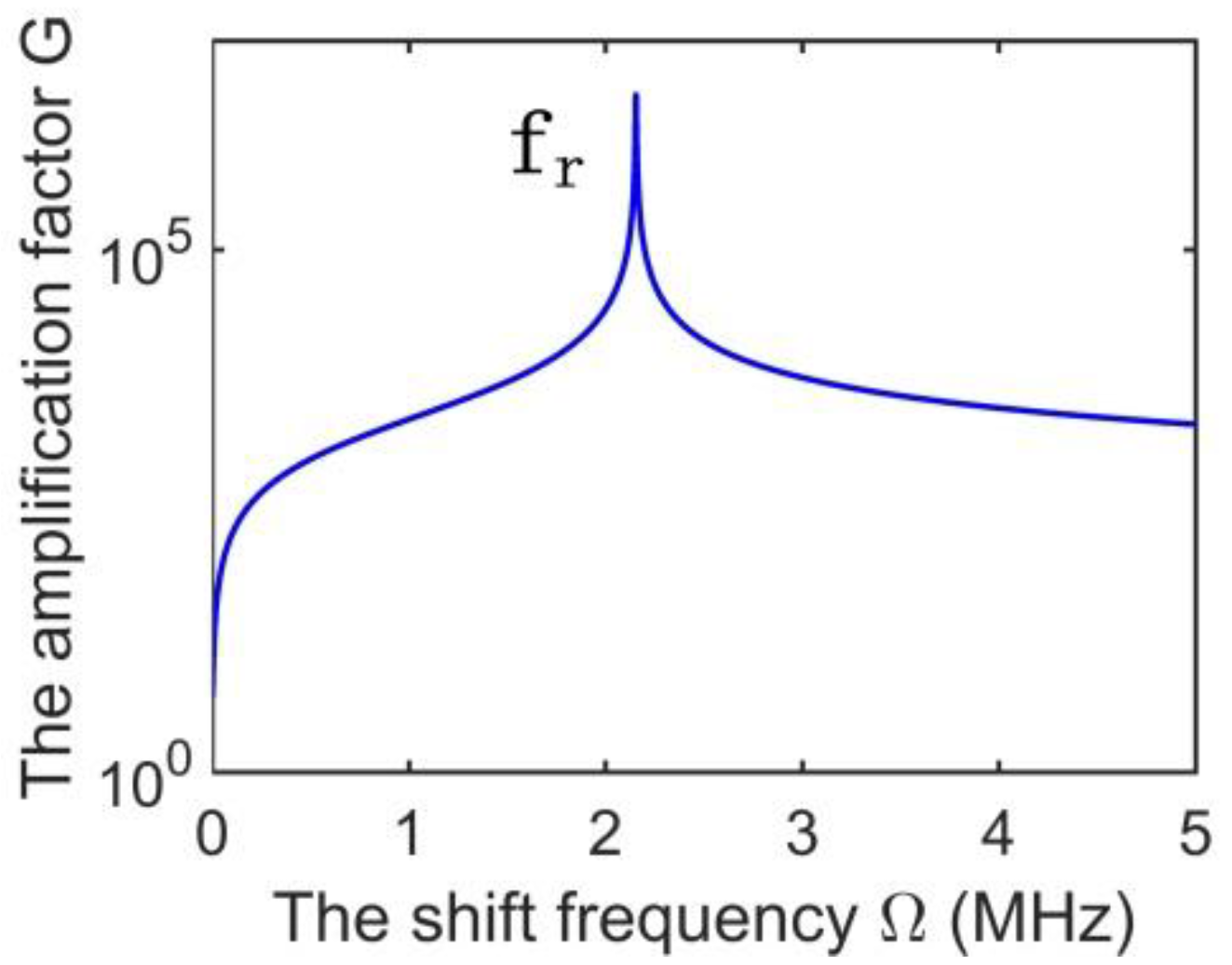
Figure 4.
Schematic diagram of the laser confocal feedback tomography. LD: laser diode; ML, microchip Nd:YVO4 laser; BS, beam splitter; PD, photodiode; L, lens; AOM1, AOM2, acousto-optic modulators; BE, beam expander; R, Reflector; Obj, objective; SA, sample (phantom); RG, radio-frequency generator; Lock-in, lock-in amplifier; PC, computer.

Figure 5.
Configuration of the quasi-common-path laser feedback interferometer. LD: laser diode; ML: microchip Nd: YAG laser; BS: beam splitter; PD: photon detector; L1, L2: lens; AOM1, AOM2: acousto-optic modulators; MR: reference mirror; T: target.
Figure 5.
Configuration of the quasi-common-path laser feedback interferometer. LD: laser diode; ML: microchip Nd: YAG laser; BS: beam splitter; PD: photon detector; L1, L2: lens; AOM1, AOM2: acousto-optic modulators; MR: reference mirror; T: target.

Figure 6.
Results of the displacement measurement: (a) phase stability test results, and (b) measurement result of PZT vibration. The bottom curve shows the PZT driving signal. (Figure reproduced from Ref. [13]).
Figure 6.
Results of the displacement measurement: (a) phase stability test results, and (b) measurement result of PZT vibration. The bottom curve shows the PZT driving signal. (Figure reproduced from Ref. [13]).

Figure 7.
Schematic diagram of the 2-D displacement measurement system. ML is the microchip laser; BS1, BS2, and BS3 are the beam splitters; L is the optical lens; AOM1, AOM2, and AOM3 are the acousto-optic modulators; R1, R2, R3, and R4, are reflectors; Iso is the optical isolator; T is the target; and PD is the photodetector. (Figure reproduced from Ref. [14]).

Figure 8.
Experimental configuration of self-mixing laser-Doppler vibrometry. LD, laser diode; APP, anamorphic prism pairs; OL, objective microscopelens; BS, glass-plate beam splitter; PD, photodiode receiver; SA, radio frequency spectrum analyzer; VA, variable attenuator; DO, digital oscilloscope; DC, frequency demodulation circuit; PC, personal computer. (Figure reproduced from Ref. [16]).

Figure 9.
(a) Power spectra (long-time average) for several applied voltages. (b) Maximum vibration amplitude versus voltage applied to the speaker. Carrier frequency, 500 kHz; modulation frequency, 8.42 kHz. (Figure reproduced from Ref. [16]).
Figure 9.
(a) Power spectra (long-time average) for several applied voltages. (b) Maximum vibration amplitude versus voltage applied to the speaker. Carrier frequency, 500 kHz; modulation frequency, 8.42 kHz. (Figure reproduced from Ref. [16]).
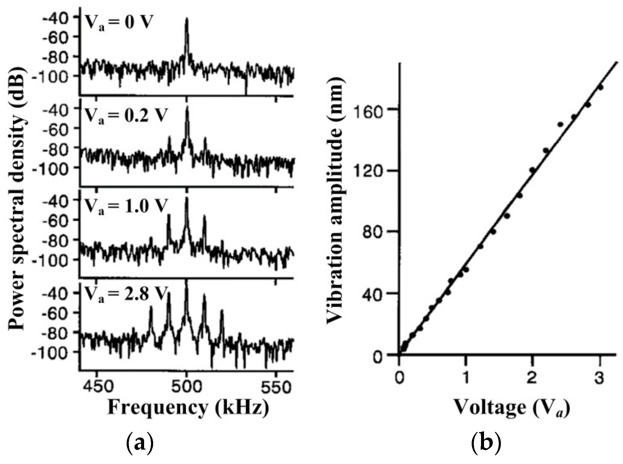
Figure 10.
(a) Experimental setup. LD, laser diode; AP, anamorphic prism pair; OL, objective lens; SL, Nd:GdVO4 solid-state laser; SG, slide glass; PD, photodiode receiver; PC, personal computer. (b) Configuration used to detect drained suspension. (Figure reproduced from Ref. [64]).
Figure 10.
(a) Experimental setup. LD, laser diode; AP, anamorphic prism pair; OL, objective lens; SL, Nd:GdVO4 solid-state laser; SG, slide glass; PD, photodiode receiver; PC, personal computer. (b) Configuration used to detect drained suspension. (Figure reproduced from Ref. [64]).

Figure 11.
(a) Power spectra of the laser output observed when the laser light is emitted into the atmosphere. Power spectra of the modulated wave observed in drained (b) 7 × 10⁻³ wt% and (c) 7 × 10⁻⁵ wt% PLS-water mixture with PLS 250 nm in diameter. (Figure reproduced from Ref. [64]).
Figure 11.
(a) Power spectra of the laser output observed when the laser light is emitted into the atmosphere. Power spectra of the modulated wave observed in drained (b) 7 × 10⁻³ wt% and (c) 7 × 10⁻⁵ wt% PLS-water mixture with PLS 250 nm in diameter. (Figure reproduced from Ref. [64]).
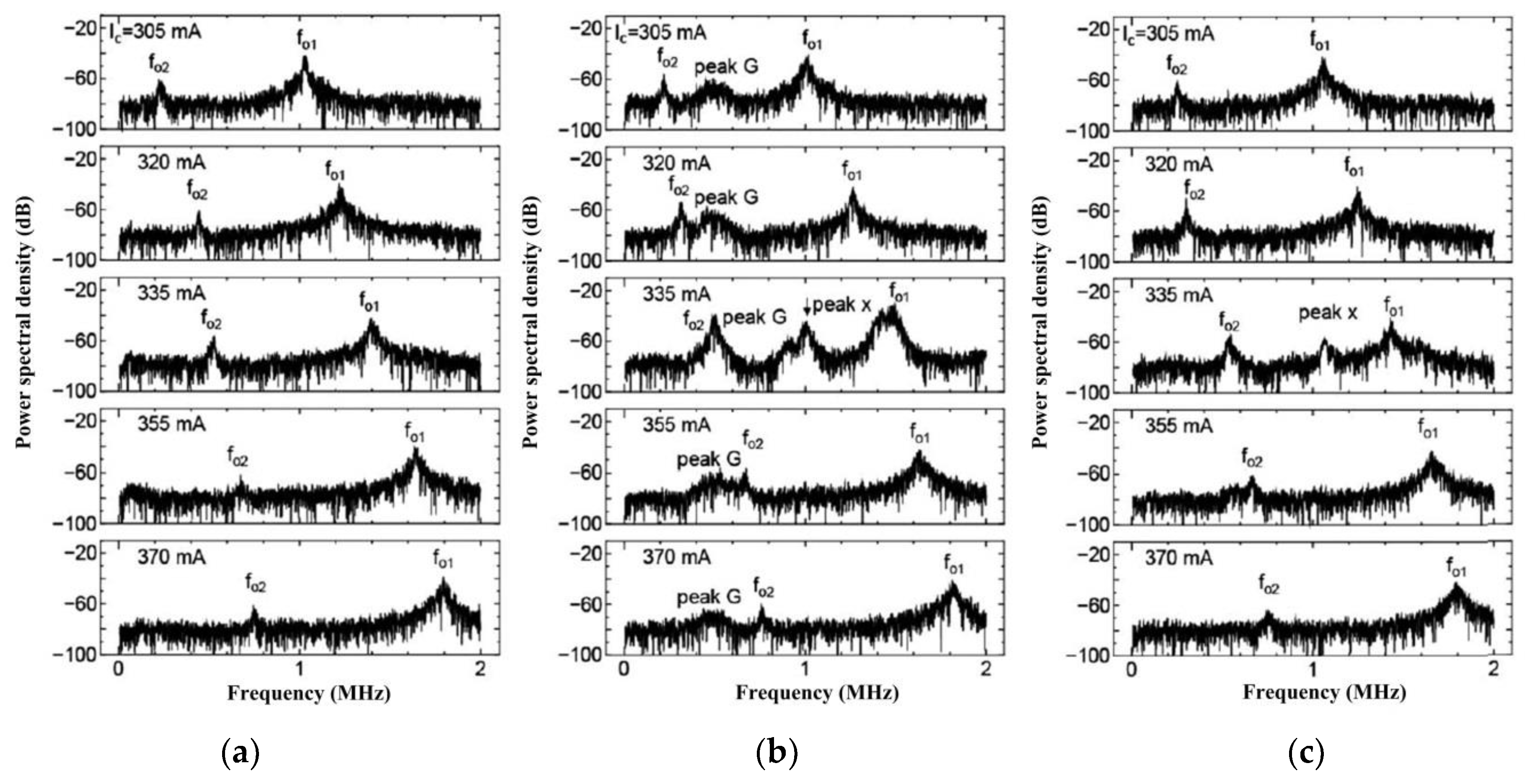
Figure 12.
Quasi-common-path laser feedback interferometer (QLFI) monitoring the liquid level. (Figure reproduced from Ref. [66]).
Figure 12.
Quasi-common-path laser feedback interferometer (QLFI) monitoring the liquid level. (Figure reproduced from Ref. [66]).
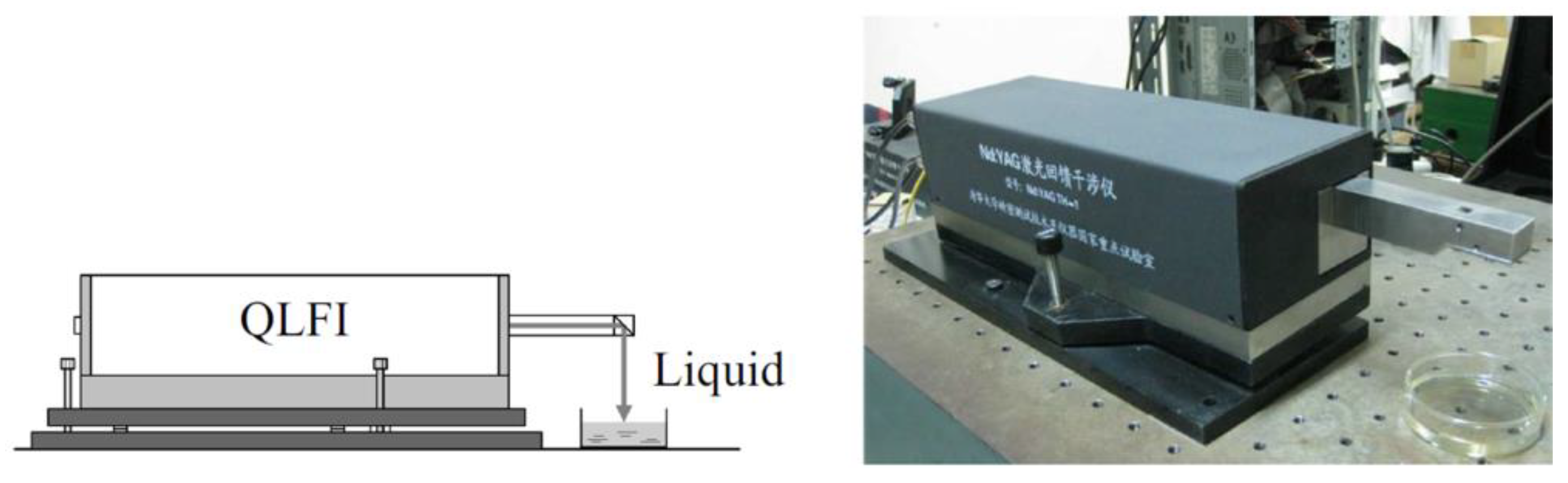
Figure 13.
Configuration of the refractive-index and thickness measurement using laser feedback interferometry. BS, beam splitter; PD, photo detector; AOM1 and AOM2, acousto-optic modulators; L, lens; Mr, reference mirror; S, sample; ME, optical wedge (measurement mirror); RF1 and RF2, radio frequency signal generators; FM, frequency mixer. (Figure reproduced from Ref. [73]).

Figure 14.
Experimental setup of the liquid refractive index measurement. LD1, LD2, laser diodes; ML1, ML2, microchip lasers; BS, beam splitter; PIN1, PIN2, detectors; AOM1, AOM2, acousto-optics modulators; L1, L2, L3, lenses; ATT, attenuator, M1, M2, MR, mirrors. (Figure reproduced from Ref. [74]).

Figure 15.
Schematic diagram of the measurement of thermal expansion coefficients based on the YAG MLFIs. YAG MLFI1 and YAG MLFI2, Nd:YAG microchip laser feedback interferometry systems; LD, laser diode; ML, microchip laser; BS, beam splitter; PD, photo detector; AOM1 and AOM2, acousto-optic modulators; L1, L2, L3, and L4, lenses; Mr1 and Mr2, reference mirrors; S, sample. (Figure reproduced from Ref. [76]).

Figure 16.
(a) Experimental system for the gear measurement; θ, rotation angle; H, eccentricity distance. (b) Experimental result with the θ = 25° and H = 20 mm.
Figure 16.
(a) Experimental system for the gear measurement; θ, rotation angle; H, eccentricity distance. (b) Experimental result with the θ = 25° and H = 20 mm.
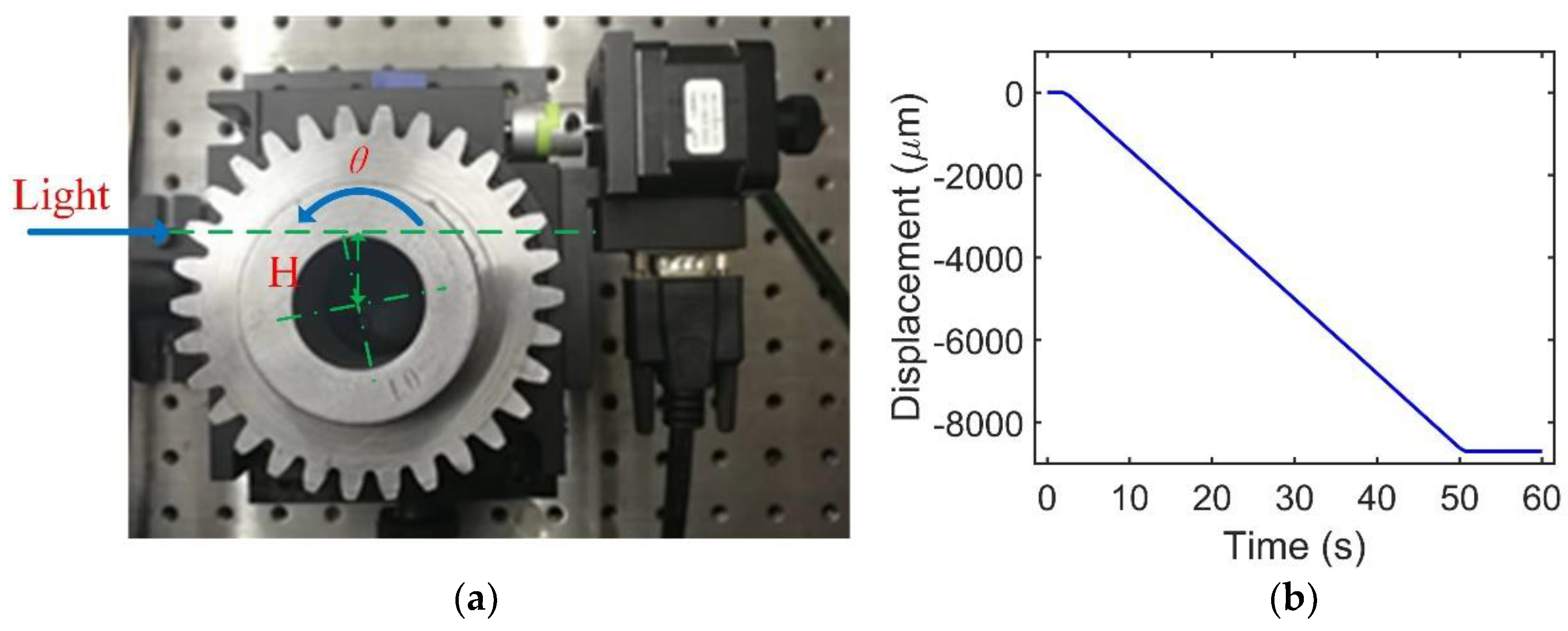
Figure 17.
Measurement of the sandwich type sample: (a) the profile of the sample, and (b) the scanning image of the sandwich type sample. (Figure reproduced from Ref. [81]).
Figure 17.
Measurement of the sandwich type sample: (a) the profile of the sample, and (b) the scanning image of the sandwich type sample. (Figure reproduced from Ref. [81]).
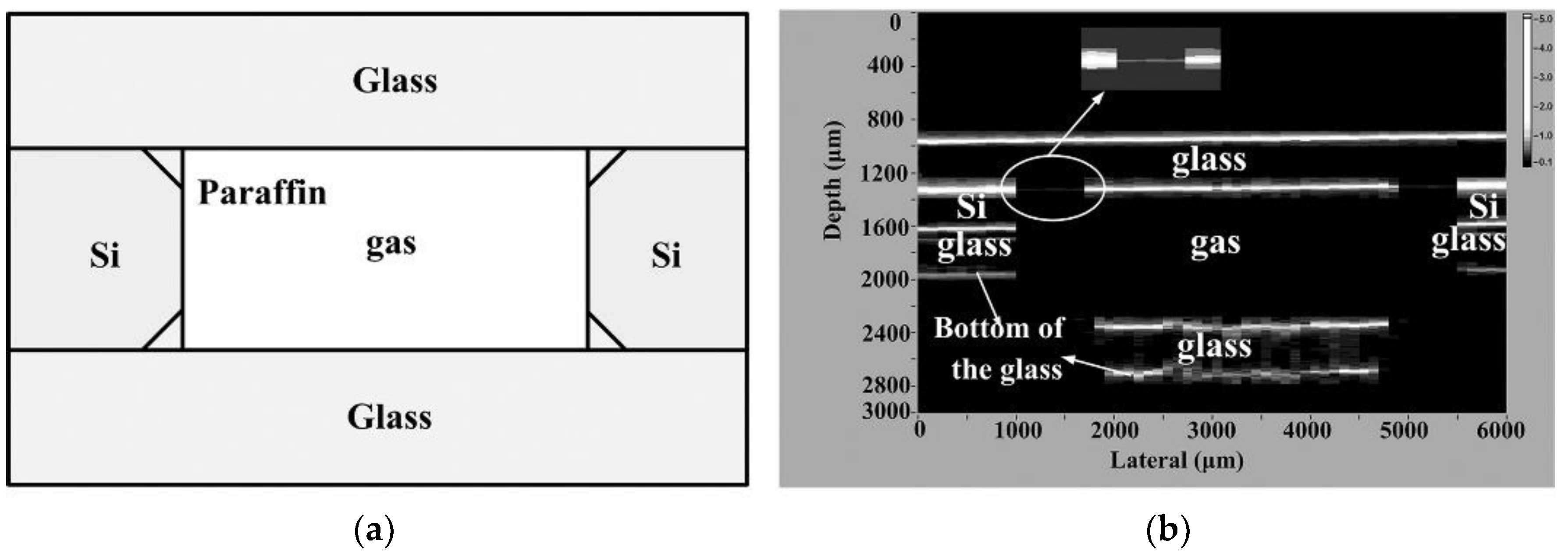
Figure 18.
Cross-sectional imaging of the pins in the onions: (a) the pin’s tip image, and (b) two parallel pin’s image. (Figure reproduced from Ref. [39]).
Figure 18.
Cross-sectional imaging of the pins in the onions: (a) the pin’s tip image, and (b) two parallel pin’s image. (Figure reproduced from Ref. [39]).
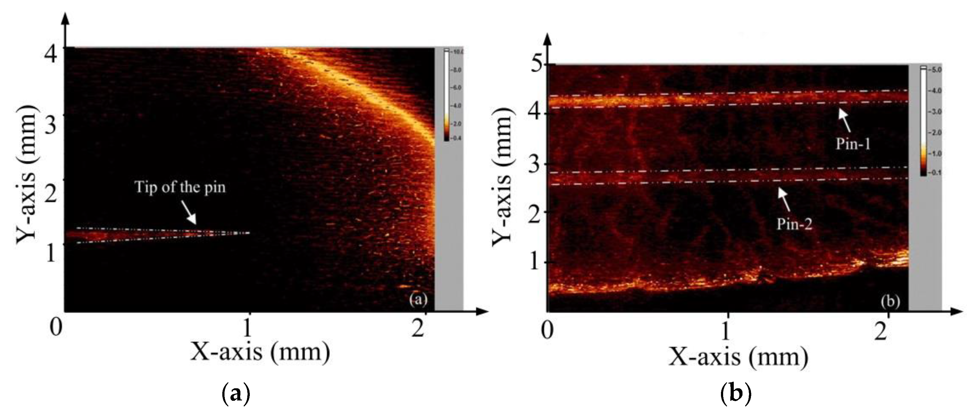
Figure 19.
(a) The normalized defocusing curve, and (b) the calibrated linear range with different objective lenses. I, NA = 0.65, II, NA = 0.55, III, NA = 0.3. (Figure reproduced from Ref. [82]).
Figure 19.
(a) The normalized defocusing curve, and (b) the calibrated linear range with different objective lenses. I, NA = 0.65, II, NA = 0.55, III, NA = 0.3. (Figure reproduced from Ref. [82]).
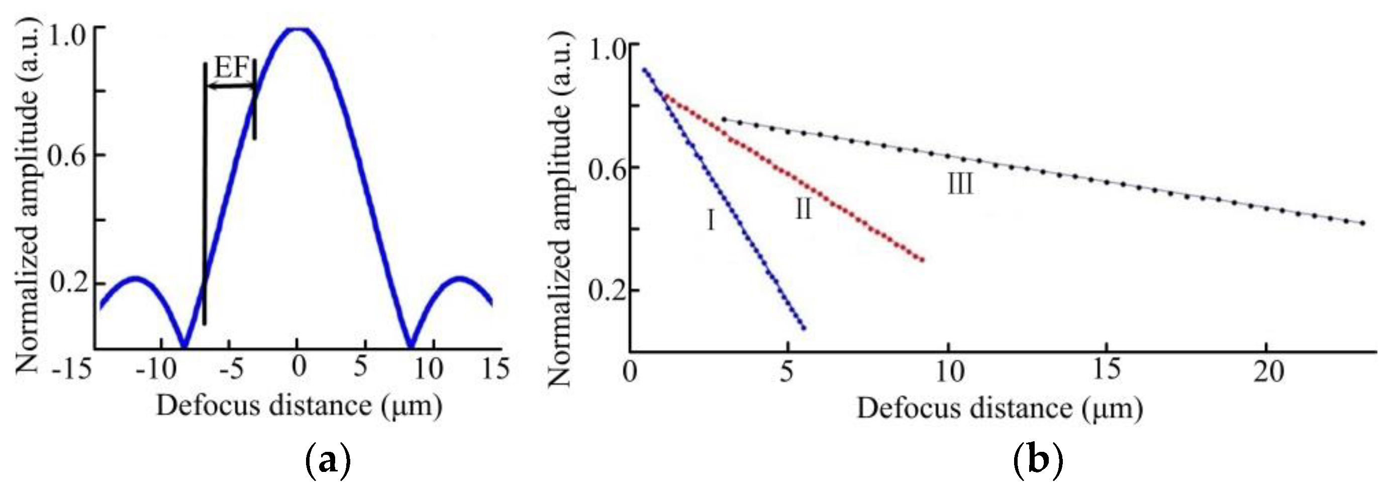
Figure 20.
(a) Physical maps of the micro-gyroscope and the rotor. (b) Measurement results of the lateral scanning. (Figure reproduced from Ref. [82]).
Figure 20.
(a) Physical maps of the micro-gyroscope and the rotor. (b) Measurement results of the lateral scanning. (Figure reproduced from Ref. [82]).

Figure 21.
Schematic of the surface measurement system. ML: microchip laser; L1–L3: lenses; BS1 and BS2: beam splitters; PD: photodiode; RF1 and RF2: reference signal generators; LIA: lock-in amplifiers; AOM1 and AOM2: acousto-optical demodulators; BE: beam expander; M1 and M2: reflect mirrors; Obj: objective lens; SA: sample; ST: stage. (Figure reproduced from Ref. [87]).
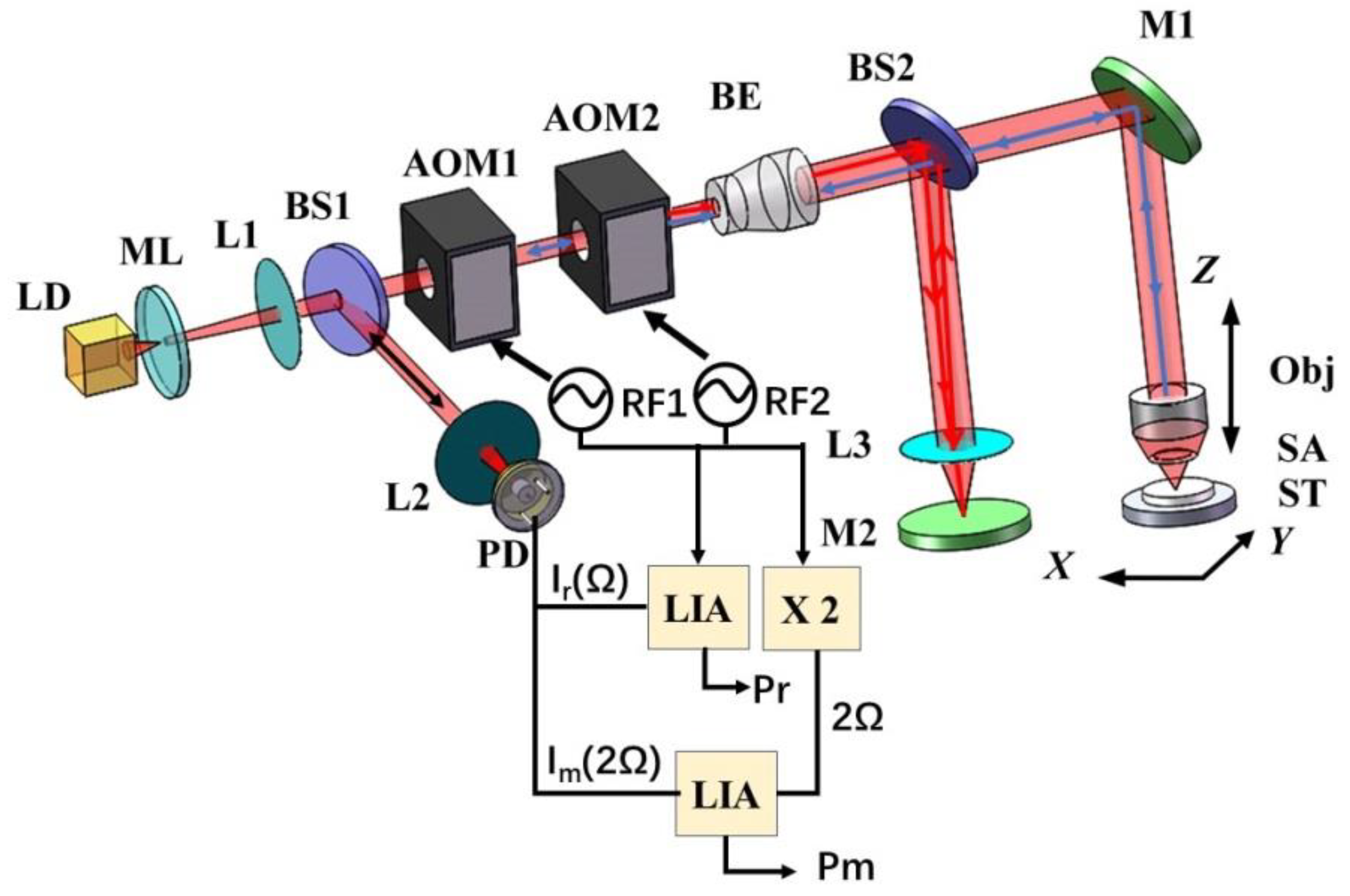
Figure 22.
Schematic of the lens thickness measurement system. LD, laser diode; Grin Lenses, graded index lenses; BS, beam splitter; AOM1 and AOM2, acousto-optic modulators; BE, beam expander; AP, annular pupil; Obj, objective lens; L, lenses; PD, photo detector; RF, reference signal generator; St, Stage; LIA, lock-in amplifier; PC, computer. (Figure reproduced from Ref. [93]).

Figure 23.
Experimental measuring results of two lenses. (Figure reproduced from Ref. [93]).
Figure 23.
Experimental measuring results of two lenses. (Figure reproduced from Ref. [93]).
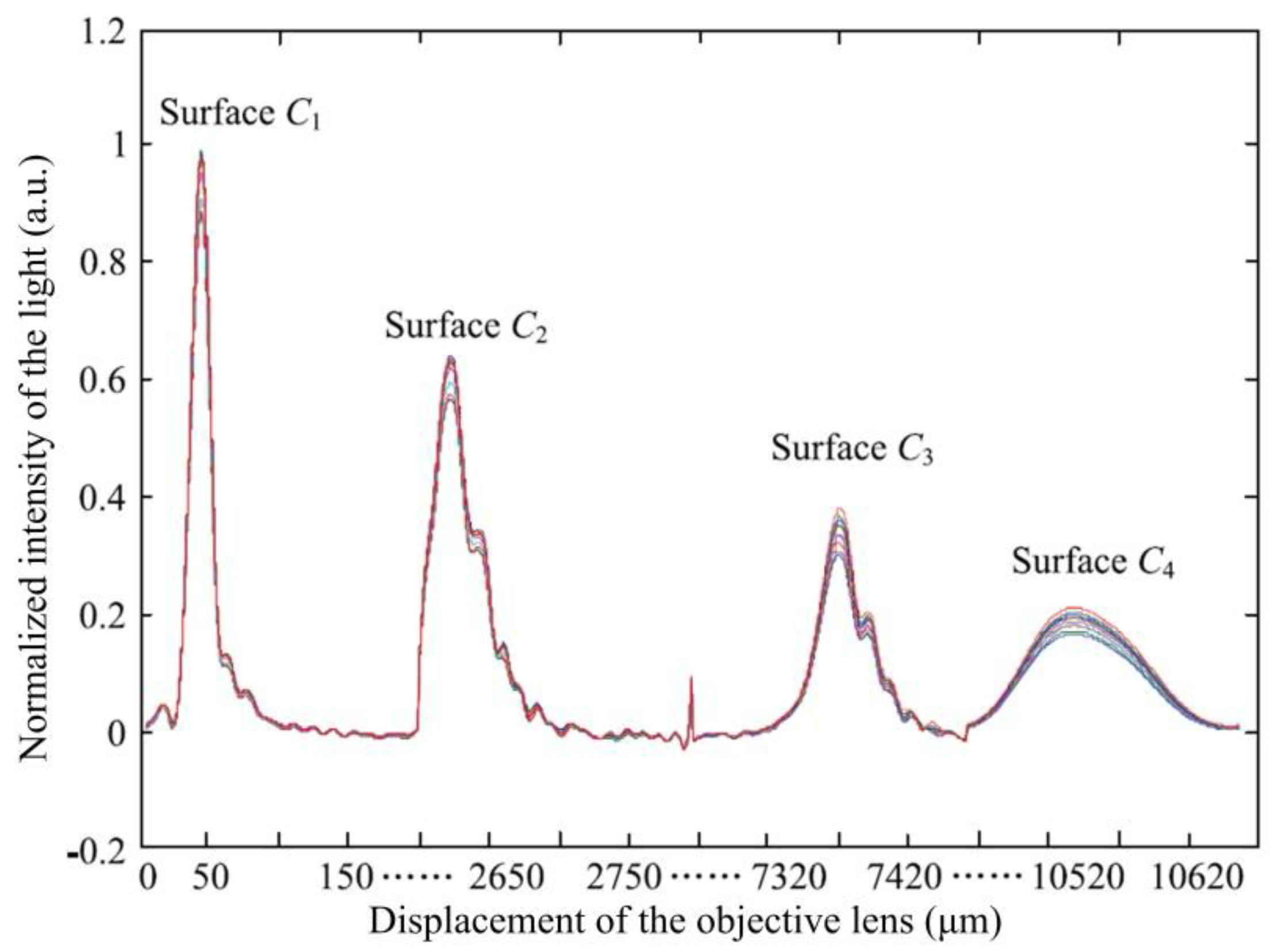
Figure 24.
Schematic diagram of the laser frequency-shifted feedback imaging system. ML, microchip laser; L1, collimator; BS, beam splitter; AOM1 and AOM2, acousto-optic modulators; L2, optical lens; Mr, reference mirror; AP, aperture; BE, beam expander; GM1 and GM2, galvanometric mirrors; L3 and L4, lenses forming the 4f system; L5, objective lens; T, target; PD, photodetector. The inset picture illustrates the physical meaning of the misalignment parameters θx and θy, where the dashed red line implies an ideal direction of the laser when θx = θy = 0. (Figure reproduced from Ref. [96]).
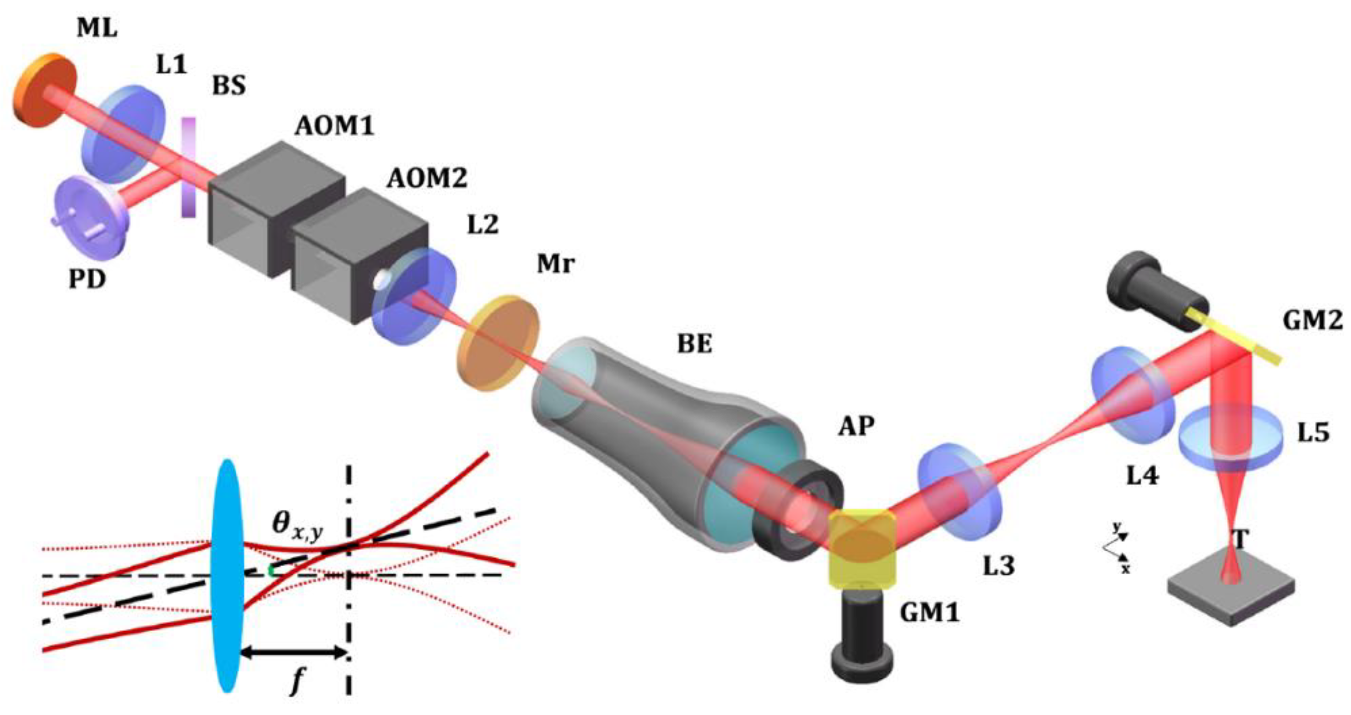
Figure 25.
Experiment results. (a) Image obtained by directly scanning. (b) Image after filtering with a DL of 48.5 mm. The three insets on the right are the magnified images that correspond to the rectangular regions labeled in the image. (c) Image after filtering with a DL of 53.5 mm. (d) Image after filtering with a DL of 58.5 mm. (Figure reproduced from Ref. [96]).
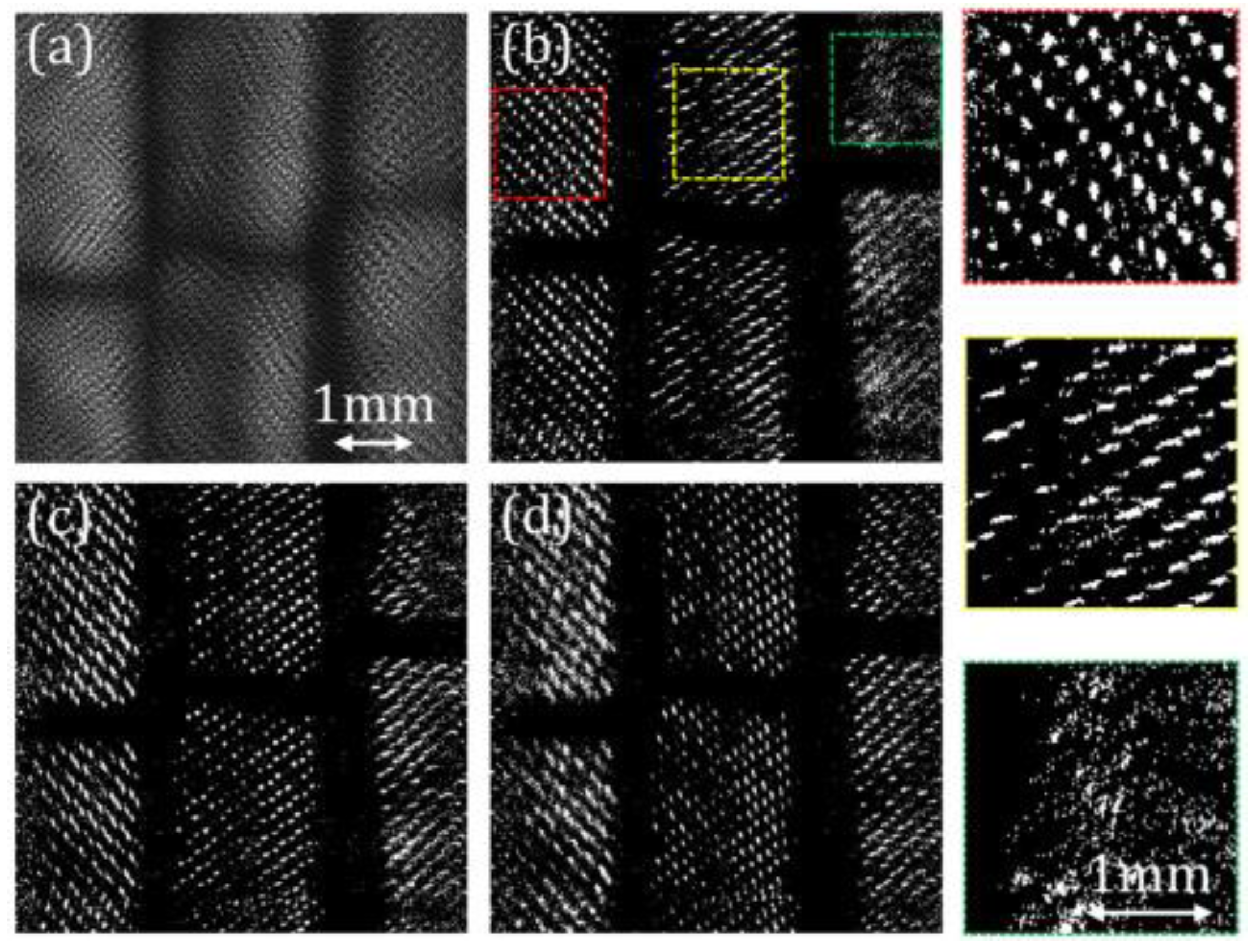
Figure 26.
Schematic diagram of the ultrasound tagged laser confocal feedback imaging system. ML, microchip Nd: YVO4 laser; BS, beam splitter; PD, photodiode; L, lens; AOM1, AOM2, acousto-optic modulators; BE, beam expender; R, reflector; Obj, objective; Sa, sample (phantom); UT, ultrasound transducer; Z, the axis of the incident light. (Figure reproduced from Ref. [97]).
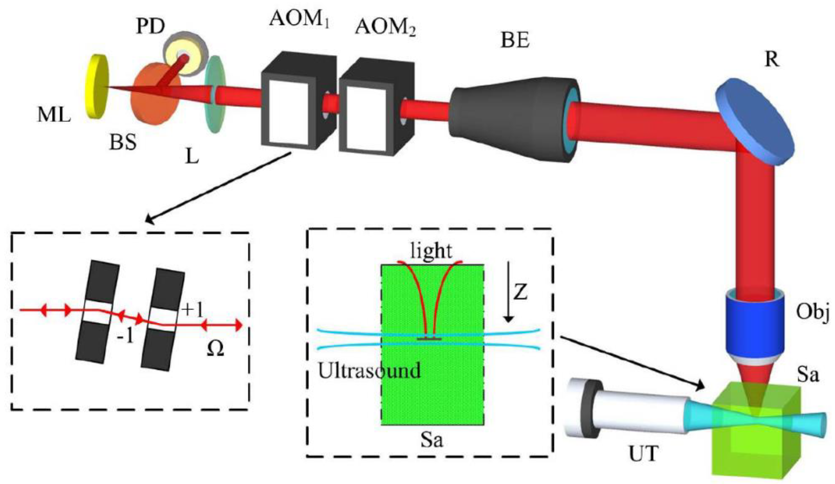
Figure 27.
Results of experimental imaging: (a) laser confocal feedback imaging, (b) ultrasound modulated laser confocal feedback imaging. (Figure reproduced from Ref. [97]).
Figure 27.
Results of experimental imaging: (a) laser confocal feedback imaging, (b) ultrasound modulated laser confocal feedback imaging. (Figure reproduced from Ref. [97]).
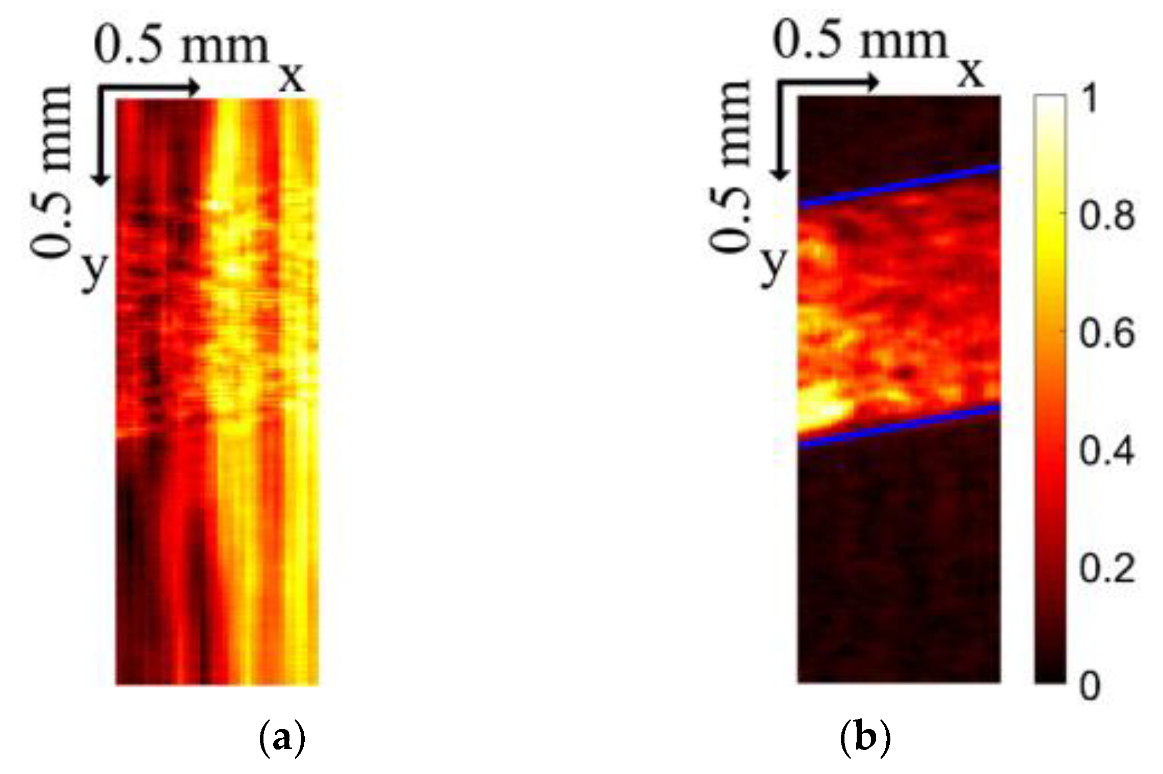
© 2018 by the authors. Licensee MDPI, Basel, Switzerland. This article is an open access article distributed under the terms and conditions of the Creative Commons Attribution (CC BY) license (http://creativecommons.org/licenses/by/4.0/).
Share and Cite
MDPI and ACS Style
Zhu, K.; Chen, H.; Zhang, S.; Shi, Z.; Wang, Y.; Tan, Y. Frequency-Shifted Optical Feedback Measurement Technologies Using a Solid-State Microchip Laser. Appl. Sci. 2019, 9, 109. https://doi.org/10.3390/app9010109
AMA Style
Zhu K, Chen H, Zhang S, Shi Z, Wang Y, Tan Y. Frequency-Shifted Optical Feedback Measurement Technologies Using a Solid-State Microchip Laser. Applied Sciences. 2019; 9(1):109. https://doi.org/10.3390/app9010109
Chicago/Turabian StyleZhu, Kaiyi, Hongfang Chen, Shulian Zhang, Zhaoyao Shi, Yun Wang, and Yidong Tan. 2019. "Frequency-Shifted Optical Feedback Measurement Technologies Using a Solid-State Microchip Laser" Applied Sciences 9, no. 1: 109. https://doi.org/10.3390/app9010109
Note that from the first issue of 2016, this journal uses article numbers instead of page numbers. See further details here.