Regular Equivalence for Social Networks

Abstract

Networks and graphs are highly relevant in modeling real-life communities and their interactions. In order to gain insight in their structure, different roles are attributed to vertices, effectively clustering them in equivalence classes. A new formal definition of regular equivalence is presented in this paper, and the relation with other equivalence types is investigated and mathematically proven. An efficient algorithm is designed, able to detect all regularly equivalent roles in large-scale complex networks. We apply it to both Barabási–Albert random networks, as well as real-life social networks, which leads to interesting insights.

1. Introduction

The availability of large datasets, derived from many sources of real-life social networks from different kinds, allows deep research into the underlying structure behind these networks. It is possible to distinguish between vertices on the basis of their local neighborhood structure in the graph, which allows one to attach a role to vertices, such that vertices with similar roles can be identified and clustered in groups. This clustering then forms a basis for higher-level analysis, focusing on the inherent structure that many social networks have in common, independent of their size, origin, or interpretation. In order to develop a full understanding of the underlying mechanics behind the interactions in a social network graph, it is also necessary to model these networks, i.e., generate artificial networks of different sizes, such that a maximum amount of observable properties of real-life networks are mimicked as well as possible.

In this work, we investigate social networks using minimal regular equivalence relations, attaching roles to vertices with a similar local neighborhood, which results in a good balance between being too strict or too loose when analyzing the network structure. The relation between minimal regular equivalence and other definitions, available in the literature, is then proven. We also introduce a fast and efficient algorithm to calculate these minimal regular equivalences, which allows researchers to quickly understand the structure of a network. We then apply our approach to both randomly generated networks as well as real-life social networks.

The paper is organized as follows. First, we provide a literature review containing references to previously published work in the field. Afterward, quite a few technical definitions are introduced, unambiguously describing our approach and positioning it with respect to other equivalence relations, through two rigorous mathematical proofs and accompanying counterexamples. This leads to the description of the regular equivalence algorithm, using pseudo-code and a proof of correctness. Closing this section is a discussion of the computational complexity of the approach. Next, the algorithm is put to the test. Apart from investigating the runtime, we use it to study randomly generated networks, culminating in a relation between the scaling exponent of the Barabási–Albert generator and the ratio of edges vs. vertices for maximal colorings. Subsequently, the algorithm is used to investigate real-life networks, which are compared with the randomly generated networks. A discussion of the results, together with an outlook to future work, closes the main body of the paper, while an appendix describes in detail the inner workings of the network generator used.

2. Background and Context

Random networks have a long history, starting with Erdos and Rényi in the late 1950s [1]. The basic idea is to generate graphs with a fixed number of vertices and afterwards adding edges, with each possible edge effectively added to the graph with fixed probability p. This approach immediately gives rise to interesting mathematical results but is inapt in modeling real-life networks [2]. Indeed, in many social networks, vertices can be grouped in relatively small clusters, a fact not observed in Erdos-Rényi random graphs. Watts and Strogatz [3] proposed a new model, which does exhibit this clustering property well and generates so-called small-world networks with weak links [4]. This model also sparked a large body of research and is successfully applied in many different contexts. However, networks generated through the procedure by Watts and Strogatz are not scale-free, a property that is sometimes observed in real-life networks: the distribution of vertex degrees in real-life networks might follow a power law [5,6,7], such that the probability that an arbitrary vertex has degree k is inversely proportional to $k^{\alpha }$ for some $\alpha >1$ called the scaling exponent. This behavior is modeled by the scale-free random network generator proposed by Barabási and Albert [8], which applies an iterative growth process combined with edge addition through preferential attachment [9,10]. Up to this date, the Barabási–Albert generator, together with its many variations, is used throughout the literature as it is the most realistic scale-free network generator available [11,12,13].

Equivalence relations, defined on the vertices of a graph, allow thorough network analysis through attaching positions or roles to vertices: the role of a vertex summarizes in some sense the structure of its neighborhood [14,15]. Attaching roles is, in effect, nothing less than identifying similarity between vertices based on the structure of surrounding subnetworks. Structural equivalence [16] and automorphic equivalence [17] are thoroughly studied in the literature, but are mathematically oriented, being defined in terms of purely graph-related definitions like automorphisms. From a practical point of view, it is more interesting to investigate looser definitions of equivalence, such as regular equivalence [18,19], which defines the role of a vertex not based on the set of its neighbors, but instead on the roles of its neighbors. This circular definition allows for a more functional approach to attaching roles to vertices and is a practical way to match the common concept of a vertex having a role in a social context.

In recent years, work has focused on theoretical investigations of social networks and the accompanying equivalences, focusing on axioms and logical characterizations [20,21,22], spectral methods [23], blocks/blockmodeling [24,25,26], and general analysis [27]. These approaches are in general much more mathematically oriented than ours, focusing on strict and rigorous scientific analysis. They have been generalized in many directions, e.g., fuzzy graphs [28], applying data-driven [29], and unsupervised role learning methods [30], some of these building upon massive amounts of data in contrast to our approach. New methods extend the ideas of equivalence through the use of additional measures when defining roles, like geodesic distance, modularity, community structure, and cliques [31,32,33], which make use of complimentary concepts beyond our definitions. Computationally, both theoretical considerations [34] as well as practical implementations have been presented [35,36,37,38].

3. Materials and Methods

This section introduces our approach in three steps: first, we exactly define some concepts, after which we introduce our regular equivalence algorithm that was specifically designed to tackle large-scale and complex networks. As a last step, we provide a proof of correctness for our approach, together with a computational complexity analysis that provides a theoretical upper bound for the calculation time.

3.1. Graphs and Equivalence Relations

In order to present our work unambiguously, we first need to introduce some classic concepts. This is necessary as, in literature, multiple (slightly different) definitions appear for these notions, sometimes leading to different conclusions which might turn out to be important to the discussion.

Definition (Graph/Network): We define a graph $G=(V,E)$ to consist of a set of vertices V and a set of edges E. An edge $e=\{u,v\}$ connects the vertices $u\in V$ and $v\in V$ and is undirected.

Throughout this paper, the vertices will be divided in groups, following several definitions all related to the concept of an equivalence relation from set theory.

Definition (Equivalence Relation): An equivalence relation $R:V\times V\to BOOL$ is a binary relation that is reflexive, symmetric, and transitive.

As is commonly known, an equivalence relation in V always induces a partition of V, which puts the vertices together in subsets of V such that every vertex is included in exactly one such subset. We write $uRv$ for two vertices u and v that are related to each other through R; they will be contained in the same subset of V in the partition of V induced by R.

In literature investigating the roles and relations of vertices in graphs or networks, one often encounters three specific equivalence relations, namely structural equivalence, automorphic equivalence, and regular equivalence, the latter having slightly differing definitions depending on the source [2,21,22,36].

Definition (Structural Equivalence): Two vertices u and v are structurally equivalent (notation: $seq(u,v)$) if and only if

$$\forall (w\in V-\{u,v\left\}\right):\{u,w\}\in E\iff \{v,w\}\in E.$$

That is, $seq(u,v)$ holds if and only if u and v have exactly the same set of neighbors, not counting the vertices u and v themselves. It is necessary to exclude u and v because otherwise two connected vertices could never be structurally equivalent.

To define automorphic equivalence, we first need to define the concept of an automorphism.

Definition (Automorphism): An automorphism of a graph is a permutation of vertices $A:V\to V$ (notation: $aut\left(A\right)$) such that edges are mapped to edges:

$$\forall (u,v\in V):\{u,v\}\in E\iff \left\{A\right(u),A(v\left)\right\}\in E.$$

Thus, an automorphism of a graph is a (possibly trivial) isomorphism of the graph and itself, hence the name.

Definition (Automorphic Equivalence): Two vertices u and v are automorphically equivalent (notation: $aeq(u,v)$) if and only if

$$\exists (A:V\to V):aut\left(A\right)\wedge A\left(u\right)=v.$$

Thus, $aeq(u,v)$ holds if and only if there exists an automorphism A that maps u to v.

The third type of equivalence relation will play an important role in this paper and is called regular equivalence. In contrast with the other two equivalence relations that were discussed above, there is no single definition of regular equivalence agreed upon in the literature. In order to define our interpretation of regular equivalence exactly, we first need to introduce additional concepts. Firstly, we have the concept of a coloring function $c:V\to \mathbb{N}$ that attaches a color (natural number) to every vertex of the graph. Coloring functions are used throughout graph theory in various contexts, like the chromatic number of a graph. Secondly, we also need the concept of a spectrum.

Definition (Spectrum): The spectrum of a vertex u under the coloring function c is the function

$$s_u:\mathbb{N}\to \mathbb{N}:n\mapsto \left|\{v\in V|\{u,v\}\in E\wedge c\left(v\right)=n\}\right|.$$

Thus, the spectrum of a vertex is a function that takes a color (natural number) as argument and returns the number of neighbors of the vertex with that color. Thirdly, we are now ready to define a regular coloring function.

Definition (Regular Coloring Function): A coloring function c is called regular (notation: $reg\left(c\right)$) if and only if

$$\forall (u,v\in V):c\left(u\right)=c\left(v\right)$$

$$\iff$$

$$\forall (n\in \mathbb{N}):\left|\right\{w\in V\left|\right\{u,w\}\in E\wedge c(w)=n\}|=|\{w\in V|\{v,w\}\in E\wedge c\left(w\right)=n\left\}\right|.$$

Thus, a regular coloring function attaches the same color to two vertices if and only if they have exactly the same distribution of colors among their respective neighbors, which can also be written using spectra as $\forall (u,v\in V):c\left(u\right)=c\left(v\right)\iff s_u=s_v$. Note that such a coloring always exists by giving each vertex a distinct color, which trivially fulfills the condition. We thus want to minimize the number of colors used in a regular coloring function, which gives rise to the fourth auxiliary definition.

Definition (Minimal Regular Coloring Function): A regular coloring function c is called minimal (notation: $minreg\left(c\right)$) if and only if

$$\forall (f:V\to \mathbb{N}):reg\left(f\right)\Rightarrow \left|\right\{n\in \mathbb{N}|\exists (u\in V):c(u)=n\}|\le |\{n\in \mathbb{N}|\exists (u\in V):f\left(u\right)=n\left\}\right|.$$

Thus, a minimal regular coloring function uses the minimal amount of colors among all regular coloring functions. Finally, we can now define regular equivalence.

Definition (Regular Equivalence): Two vertices u and v are regular equivalent (notation: $req(u,v)$) if and only if

$$\forall (c:V\to \mathbb{N}):minreg\left(c\right)\Rightarrow c\left(u\right)=c\left(v\right).$$

Thus, u and v need to have the same color for all minimal regular coloring functions. The algorithm that is presented in this paper will prove that the minimal regular coloring is uniquely defined for a graph, and thus an equivalent definition could have been that two vertices are regular equivalent if and only if $\exists (c:V\to \mathbb{N}):minreg\left(c\right)\wedge c\left(u\right)=c\left(v\right)$. We are aware that other definitions of regular equivalence are used throughout the literature, but for the entirety of this paper we will adhere to the one defined above.

As we have seen, multiple equivalence relations can be defined upon a graph. These different relations have interdependencies to each other, in the sense that some equivalence relations are more strict than others.

Definition (Strictness): For two equivalence relations $R_1$ and $R_2$, we say that $R_1$ is more strict than $R_2$ (notation: $R_1\prec R_2$) if and only if

$$\forall (u,v\in V):u{R}_{1}v\Rightarrow u{R}_{2}v.$$

It is now possible to prove that structurally equivalent vertices are also automorphically equivalent, but not necessarily vice versa. Additionally, automorphically equivalent vertices are regularly equivalent, but not necessarily vice versa. Stated otherwise, there is a clear ordering between the 3 equivalence definitions, which we now demonstrate through the following two proofs. We start by proving the relation between structural and automorphic equivalence.

Theorem 1.

Structural equivalence is more strict than automorphic equivalence

Proof. 

Consider a structural equivalence relation R. It is sufficient to demonstrate that an automorphism of the graph exists with $A\left(u\right)=v$ and $A\left(v\right)=u$, given $uRv$. Given that the neighbors of u and v are the same, possibly excepting u and v themselves, it is trivial to take the automorphism $A:V\to V$ such that

$$A\left(w\right)=\left\{\begin{array}{cc}v\hfill & \mathrm{if}w=u,\hfill \\ u\hfill & \mathrm{if}w=v,\hfill \\ w\hfill & \mathrm{otherwise}.\hfill \end{array}\right.$$

 □

In order to demonstrate that structural equivalence and automorphic equivalence are different concepts, we need to provide a counterexample: a graph containing two vertices u and v that are automorphically equivalent but not structurally equivalent. This can be done easily. A graph with four vertices which are linearly connected to each other in a single chain is sufficient, as the two outer vertices have different neighbors but are still automorphically equivalent.

We continue by proving the relation between automorphic and regular equivalence.

Theorem 2.

Automorphic equivalence is more strict than regular equivalence

Proof. 

We need to prove that $\forall (u,v\in V):aut(u,v)\Rightarrow reg(u,v)$. Consider an automorphic equivalence relation R and consider any two vertices $u,v\in V$ such that $uRv$, that is, there exists an automorphism $A:V\to V$ such that $A\left(u\right)=v$. We now need to prove that the minimal regular coloring function attaches the same color to u and v. We will first prove that the coloring corresponding to R is a regular coloring function.

Consider the coloring function $c:V\to V$ such that $\forall (u,v\in V):uRv\iff c\left(u\right)=c\left(v\right)$. We will now prove that $s_u=s_v$, that is, u and v have the same spectrum. Indeed, as A is an automorphism of the graph, every neighbor $w_u$ of u will be mapped by A to some neighbor $w_v$ of v; formally, $\forall (w_u\in V):\{u,w_u\}\in E\Rightarrow \exists (w_v\in V):A\left(w_u\right)=w_v\wedge \{v,w_v\}\in E$. Thus, there exists an automorphism that maps $w_u$ to $w_v$, namely A itself; thus, $w_{u}R{w}_v$ and thus $c\left(w_u\right)=c\left(w_v\right)$. We have thus proven that we can map any neighbor $w_u$ of u to a neighbor $w_v$ of v while preserving the color. This is tantamount to saying that the spectrum $s_u$ is equal to the spectrum $s_v$. Thus, the coloring function c is indeed a valid regular coloring function and $c\left(u\right)=c\left(v\right)$.

Now, although c is a valid regular coloring function, it still might be the case that it does not use the minimal number of colors; that is, it might not be a minimal regular coloring function. However, changing the regular coloring function c to a minimal regular coloring function $c^{\prime }$ involves attaching the same color to vertices that previously had a different color, because their spectrum is the same (although no automorphism exists that maps them to each other). Thus, $\forall (u,v\in V):reg\left(c\right)\wedge minreg\left(c^{\prime }\right)\wedge (c\left(u\right)=c\left(v\right))\Rightarrow (c^{\prime }\left(u\right)=c^{\prime }\left(v\right))$. This concludes our proof, as we already demonstrated that $c\left(u\right)=c\left(v\right)$. □

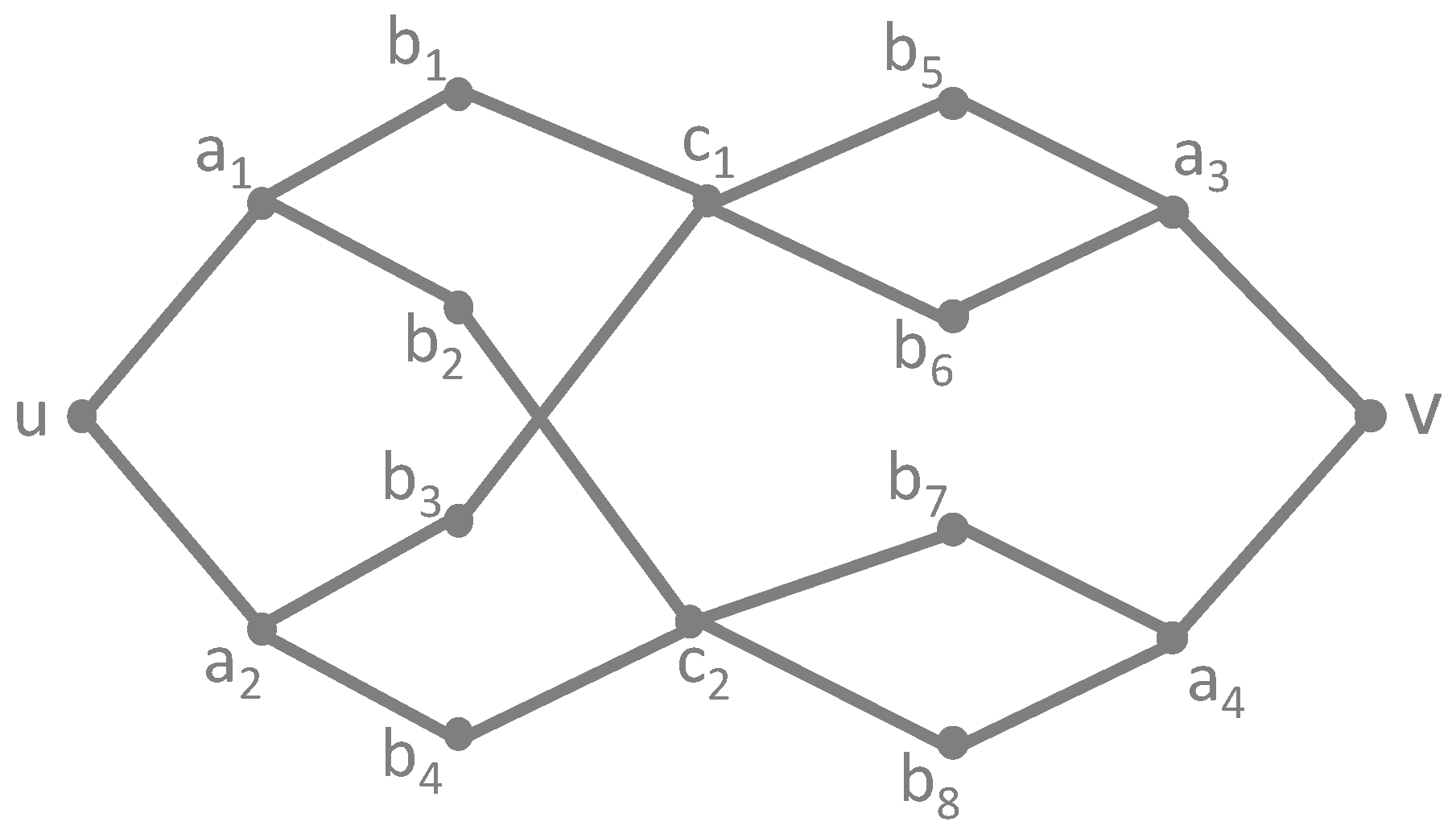
In order to demonstrate that automorphic equivalence and regular equivalence are different concepts, we need to provide a counterexample: a graph containing two vertices u and v that are regularly equivalent but not automorphically equivalent. Such a graph is more difficult to construct, and one example is given in Figure 1.

As strictness is transitive, we immediately obtain that structural equivalence is more strict than regular equivalence. In practice, both structural equivalence and automorphic equivalence are very strict when applied to real-life social networks, having only very little vertices being equivalent to each other. Indeed, two vertices are structurally equivalent if and only if they have exactly the same set of neighbors (excluding themselves), which is something that rarely happens in real-life networks. Additionally, two vertices are automorphic equivalent if and only if the connections of the whole, global graph look exactly the same from their respective points of view, which is what automorphic equivalence expresses informally. Thus, little structure is discovered when investigating these networks using only structural equivalence and automorphic equivalence. In contrast, regular equivalence is much “looser,” allowing more structure to be discovered, with more vertices being equivalent to each other. Thus, regular equivalence is an important tool that allows us to gain additional insight in network structure. It does not require neighbors to be exactly the same vertices, as it is sufficient that neighbors have the same role. Additionally, it takes into account the local connection-structure of the vertices instead of the global structure, which is once more relaxing the condition for vertices to be equivalent. It is thus possible to investigate the structure without having to look at too fine-grained details, discovering meaningful relations or roles between the vertices.

3.2. Regular Equivalence Algorithm

In order to compute the regular equivalence relation for a graph, we now present an algorithm that iteratively partitions the vertices in different groups. As we are looking for a coloring function that uses a minimal number of colors, we start by attaching the same color to all vertices, and iteratively add new colors to vertices that definitely cannot have the same color. This is determined through the use of the spectrum of a vertex, which shows how many vertices of each color are adjacent to the current vertex under scrutiny. The spectrum thus functions as a blueprint of the neighborhood of a vertex.

3.2.1. Description of the Algorithm

We now continue with a description of the algorithm. In short, we start with all vertices in one set, and iteratively split up this set in more sets, such that vertices that do not have the same spectrum are put in different sets, effectively building a partition of all vertices in each step. The algorithm stops when no vertices need to be separated from each other anymore, that is: each set in the partition only contains vertices that have the same spectrum.

As we are going to repeatedly calculate and update the spectra of the vertices, we need a function that keeps track of these spectra and groups the vertices with the same spectrum together, and effectively calculates the partition. We denote this partition-building function by p, and this p takes a spectrum $s_u$ as input, i.e., a function $\mathbb{N}\to \mathbb{N}$, and returns the set of vertices that have the same spectrum i.e., $\{v\in V|s_u=s_v\}$. This subset of V, which of course contains u itself, is an element of the powerset of V (notation: $2^V$ or $\mathcal{P}\left(V\right)$) and we can thus formally write down $p:(\mathbb{N}\to \mathbb{N})\to 2^V:s_u\mapsto \{v\in V|s_u=s_v\}$. It is key to our approach that the partition-building function p can be calculated efficiently.

We now have all ingredients to discuss the algorithm that calculates the regular equivalences. We first initialize the color of all vertices to the same temporary color, the number zero. In the repeat-loop, we will calculate the spectra of the vertices under this coloring, and split up vertices that have a different spectrum but still received the same temporary color during the previous iteration. We thus introduce additional colors when the need arises and update the coloring function accordingly. In this repeat-loop, we build up a new partition and initialize the partition to be the empty set. We then calculate the spectrum $s_u$ for all vertices u and group together the vertices with the same spectrum. After all vertices have been processed, the partition-building function p will actually exhibit a number of nonempty subsets of V, such that each $u\in V$ is contained in exactly 1 of these subsets, i.e., p will correspond to a partition. If this number of nonempty subsets is equal to the number of colors used in the previous iteration, this means that no colors have been updated since then and that no vertices u and v with the same color but a different spectrum have been encountered. We thus found a minimal regular equivalence coloring and can break the repeat-loop.

Otherwise, we remember the number of colors used in this iteration, and start updating the colors of the vertices. This is done by iterating over all subsets in the partition, and attaching the same color to all vertices in such a subset, starting with zero and incrementing the value of the color for each subset processed. After finishing the repeat-loop, the algorithm returns the minimal regular coloring function c, from which it is easy to derive the regular equivalence relation: two vertices u and v are regular equivalent if and only if they have the same color, i.e., $c\left(u\right)=c\left(v\right)$.

Algorithm 1 Regular equivalence.

Input: Graph G Output: Minimal regular coloring function c 1:  for $u\in V$ do $c\left(u\right)\leftarrow 0$ end for 2:  $ColorsUsed\leftarrow 1$ 3:  repeat 4:      for $s\in \mathbb{N}\to \mathbb{N}$ do $p\left(s\right)\leftarrow \varnothing$ end for 5:      for $u\in V$ do 6:          Calculate $s_u$ 7:          $p\left(s_u\right)\leftarrow p\left(s_u\right)\cup u$ 8:      end for 9:      if $\left|\right\{s\in \mathbb{N}\to \mathbb{N}\left|p\right(s)\ne \varnothing \}|=ColorsUsed$ then 10:        break repeat-loop 11:     end if 12:     $ColorsUsed\leftarrow \left|\right\{s\in \mathbb{N}\to \mathbb{N}\left|p\right(s)\ne \varnothing \}|$ 13:     $CurrentColor\leftarrow 0$ 14:     for $x\in \{p\left(s_u\right)\in 2^V|u\in V\}$ do 15:         for $y\in x$ do $c\left(y\right)\leftarrow CurrentColor$ end for 16:         $CurrentColor\leftarrow CurrentColor+1$ 17:     end for 18:  end repeat 19:  return c

This (mathematical) pseudocode leaves many choices for a practical implementation. The most important decision concerns the use of the datastructure for the partition-building function p. Our implementation uses a generic map-object. As such, the instruction for $s\in \mathbb{N}\to \mathbb{N}$ do $p\left(s\right)\leftarrow \varnothing$ corresponds to $p.clear\left(\right)$, the instruction $p\left(s_u\right)\leftarrow p\left(s_u\right)\cup u$ corresponds to $p.get\left(s_u\right).add\left(u\right)$, and the value $\left|\right\{s\in \mathbb{N}\to \mathbb{N}\left|p\right(s)\ne \varnothing \}|$ corresponds to $p.size\left(\right)$. Moreover, the for-loop over $x\in \{p\left(s_u\right)\in 2^V|u\in V\}$ corresponds to a loop over all $p.values\left(\right)$ and $y\in x$ is of course also implemented as a loop over x.

3.2.2. Proof of Correctness

We now prove the correctness of the above algorithm to calculate the regular equivalence relation. First, we need to prove that the coloring function is indeed a regular coloring function; i.e., two vertices have the same color if and only if they have the same spectrum. Second, we need to prove that this coloring is indeed minimal, i.e., that it uses a minimal number of colors. Third, we need to prove that the solution is reached eventually, i.e., that the algorithm will always terminate.

Theorem 3.

The regular equivalence algorithm calculates the minimal regular coloring function

Proof. 

The algorithm starts with attaching the same color to all vertices. It then repeatedly calculates all spectra; it groups together the vertices with the same spectra and separates vertices with different spectra by assigning a different color to them. If two vertices have the same spectrum, then the algorithm will assign the same color to them. If two vertices have a different spectrum, then the algorithm will assign a different color to them. This proves the first part of the theorem.

Secondly, it is never possible that two vertices with different colors should receive the same color again, as they already received a different color in a previous iteration due to the fact that they were already determined to have a different spectrum at that point. Indeed, introducing more colors can never simplify the spectrum of any vertex; the total number of colors present in the spectrum of a vertex can never decrease. The algorithm only introduces additional colors if needed; i.e., two vertices were identified with different spectra but had the same color, so they have to be separated. Thus, the algorithm will always use a minimal number of colors. This proves the second part of the theorem.

Thirdly, we start with assigning the same color to all vertices. In every iteration, at least one additional color is introduced; otherwise, the algorithm stops iterating. At most $\left|V\right|$ colors will be used, when all vertices receive a different color. At that point, the iteration stops because the number of colors used stays the same. Thus, in a finite number of steps, the algorithm will always terminate and return. □

3.3. Computational Complexity

Next, it is necessary to investigate the computational complexity of the algorithm at hand. Lines 1 and 2 are $O\left(\right|V\left|\right)$ and constant time respectively. An upper bound for the repeat-loop can be easily established as at least one color is added each iteration, with a maximum of $\left|V\right|$ colors. In Line 4, we initialize the partition-building function p, which can be done in constant time. The spectrum of a vertex can be calculated in linear time through the use of adjacency-lists, a standard implementation technique for graphs [39]. Adding the vertex u to the partition-building datastructure can be done in constant time. Calculating the number of sets in the partition (Lines 9 and 12) can be done in constant time, just like Line 13. Lines 14 and 15 together iterate over all vertices once ($O\left(\right|V\left|\right)$): each vertex gets assigned its new color. Line 16 is executed at most $\left|V\right|$ times and takes a constant time. Taking everything together, the total computational complexity is $O\left(\right|V{|}^2)$, as the repeat-loop in Line 3 combined with the iteration over all vertices in Lines 14 and 15 is the most significant part in the analysis.

4. Results

In this section, we present experimental results using real-life social graphs and complex graphs obtained using a generalized Barabási–Albert random network generator, described in Appendix A.

4.1. Runtimes for Calculating Regular Equivalences

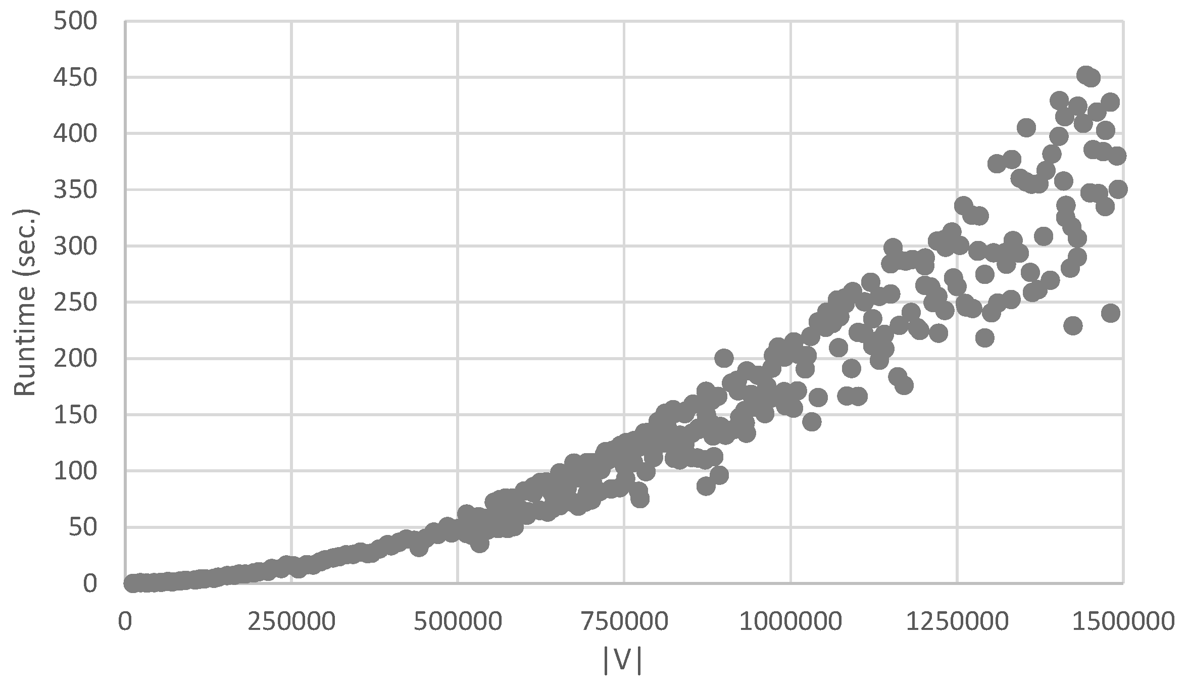
First of all, we investigate practical running times for calculating regular equivalences. We generated 350 random complex networks (using the algorithm in Appendix A), having ${10}^4\le \left|V\right|\le 1.5\times {10}^6$ vertices, each having $3\left|V\right|\le \left|E\right|\le 15\left|V\right|$ edges, which is representative for the real-life social networks studied in this paper. We then calculated the minimal regular equivalence relation using the algorithm above, and timed the execution, using Java 1.8.0_60 (x64) on an Intel Core i7-5600U 2.6 GHz with 16 GB RAM. Results can be seen in Figure 2. The quadratic polynomial $y\left(x\right)={10}^{-10}{x}^2+4\times {10}^{-5}x$ was fitted to the data with a coefficient of determination $R^2=0.93$, which means that the experimental values are statistically well explained by the quadratic polynomial. For an average randomly generated graph, the repeat-loop was executed only about four times, which explains the fact that the execution time is very low, although the computational complexity was shown to be quadratic in theory. Moreover, it turns out that for real-life social networks the execution time is very low as well. Our approach is thus a valid way to investigate real-life, large-scale, and complex networks, allowing deep analysis which was previously very demanding with respect to the required computational time.

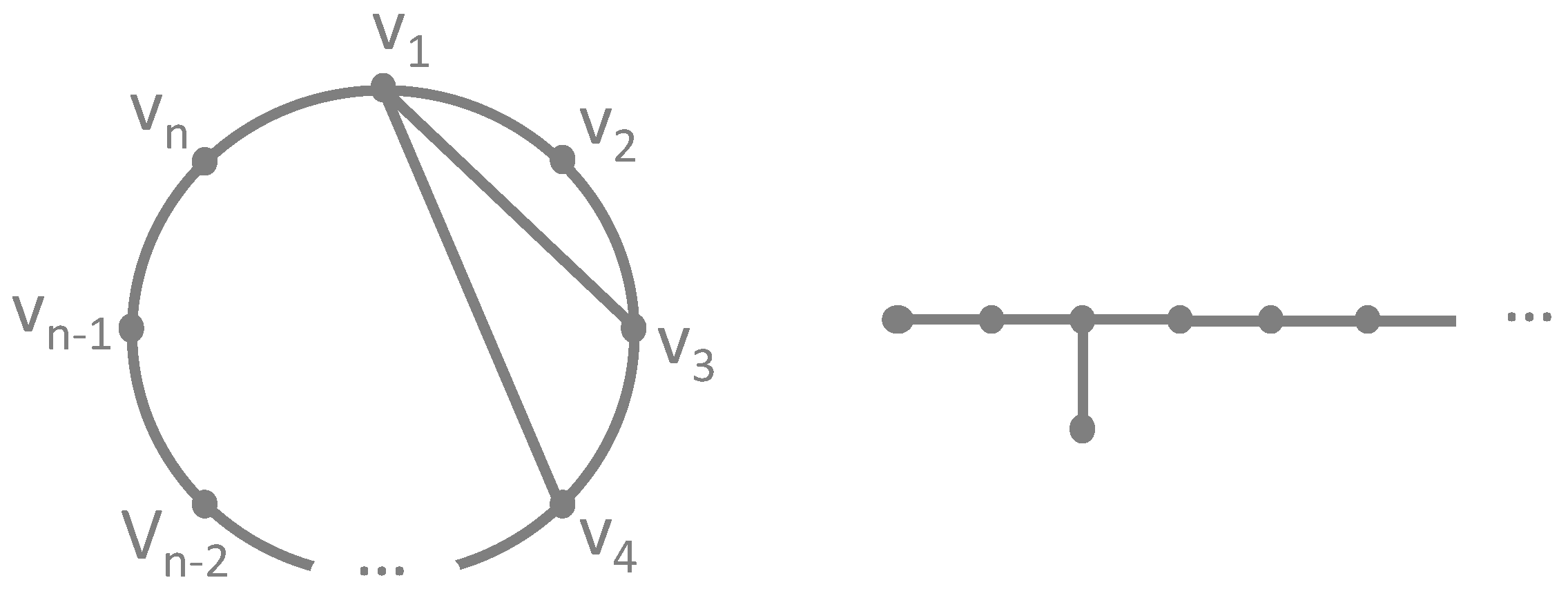
However, it is quite possible to construct a graph that needs $O\left(\right|V\left|\right)$ iterations, resulting in the maximum number of colors $\left|V\right|$ needed for the minimal regular coloring. Two such graphs are shown in Figure 3. For example, take some $n\in \mathbb{N}$ such that $6\le n$, then one can define the circular graph on the left of Figure 3 as $G=(V,E)$ with $V=\{v_i\in \mathbb{N}|1\le i\le n\}$ and $E=\left\{\{v_i,v_{i+1}\}\right|1\le i<n\}\cup \{\{v_n,v_1\},\{v_1,v_3\},\{v_1,v_4\}\}$. The algorithm will then need $O\left(\right|V\left|\right)$ iterations, after which all vertices will have received a unique color. A second example is shown on the right of Figure 3. The key to understanding that the algorithm takes many iterations in these cases follows from the fact that the vertices receive a new color one by one, each iteration changing the spectrum of only 2 other vertices (the neighbors). As such, the algorithm has to propagate through the graph linearly and that takes $O\left(\right|V\left|\right)$ iterations. Clearly, these two examples are fabricated and do not likely appear in real-life, making them pathological situations with which we are able to stress-test the algorithm.

4.2. Experiments

In this section, we will investigate properties of complex large-scale networks related to the minimal regular equivalence relation. We will investigate, for both random graphs obtained by a Barabási–Albert generator as well as for real-life social graphs, the minimal regular coloring function and the accompanying minimal regular equivalence relation. More specifically, we will look in detail at the number of colors required by such a minimal regular coloring function, and how this number evolves in relation to the size of the network.

First, we will look into randomly generated complex networks, and see how the required number of colors grows with respect to the size of the graph. We then will apply the algorithm to large-scale real-life social networks and interpret the results.

4.2.1. Random Barabási–Albert Graphs

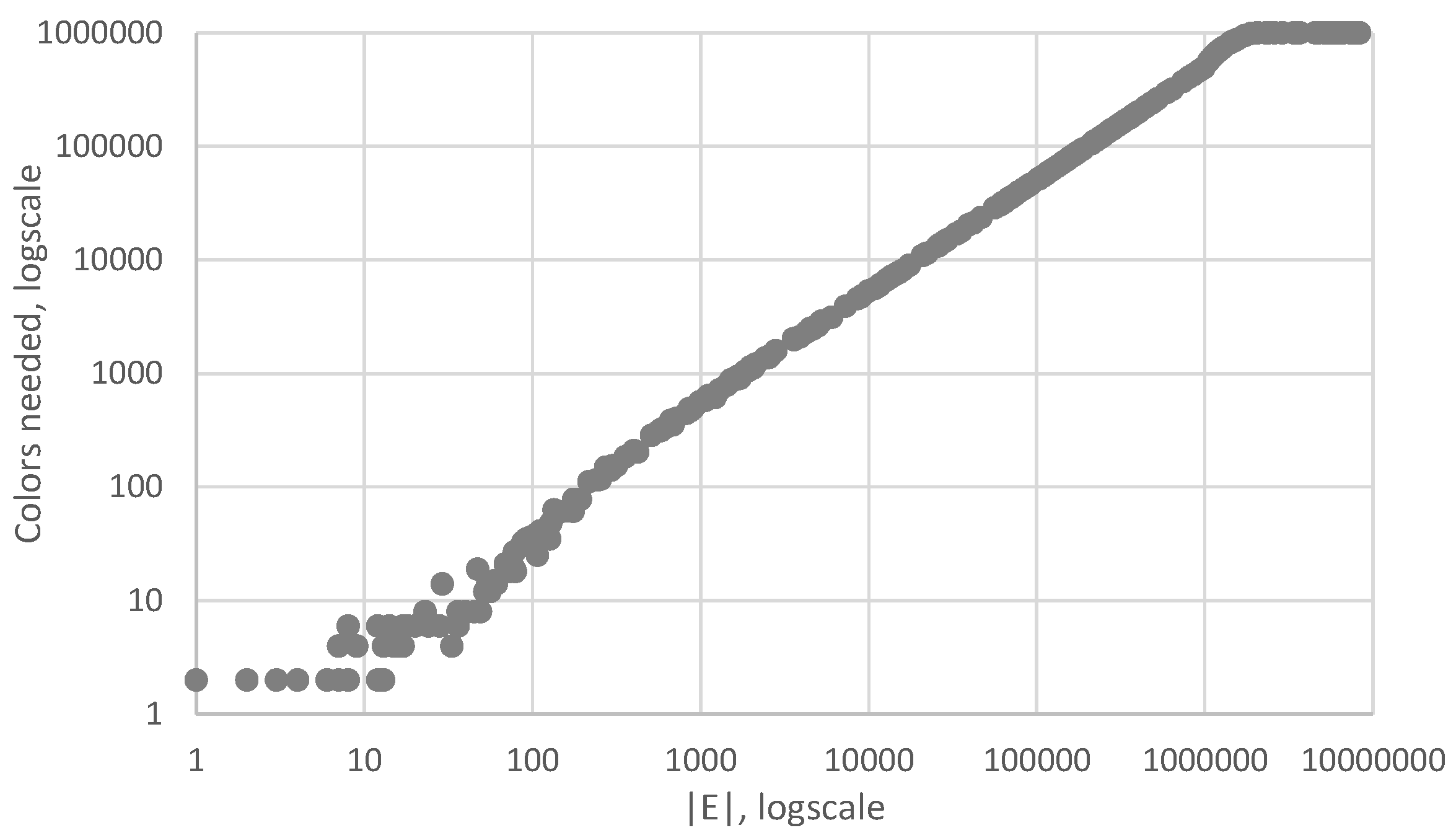
As a first experiment, we will investigate how the number of required colors for a minimal regular equivalence coloring grows in function of the number of edges in a graph. To that aim, we will generate 350 scale-free graphs, each having $\left|V\right|={10}^6$. However, each of these graphs will have a different number of edges, randomly generated such that $1\le \left|E\right|\le {10}^7$. These edges are distributed in a scale-free way, through the use of a Barabási–Albert graph generator with appropriate parameters, most important with scaling exponent $\alpha =3$ (see Appendix A for details). For each of these random graphs, we computed the minimal regular equivalence relation and obtained a minimal number of colors; see Figure 4. On average, one such experiment took a few minutes.

As can be expected, graphs with very low numbers of edges need only a very low number of colors, i.e., only a very small number of different spectra is obtained. As the number of edges in the graph grows, so does the number of colors needed. Note that both axes are logarithmically scaled in order to present the results in a clear way.

Note the flat top in the graph, occurring around $\left|E\right|\approx 2\times {10}^6$. At that point, we need ${10}^6$ colors, i.e., the maximum number of colors available as every vertex gets its own color (no color is used twice). We can conclude that, once a random graph contains a certain number of edges, the vertices are sufficiently connected to each other such that typically no two vertices have the same spectrum. If we continue adding edges, i.e., ${10}^7\ll \left|E\right|$ (not depicted in the graph), we can expect the number of colors needed in the long run to finally drop again, up until once again only one color is needed, in the case of a complete graph with $\left|E\right|=\left|V\right|\ast \left(\right|V|-1)/2$.

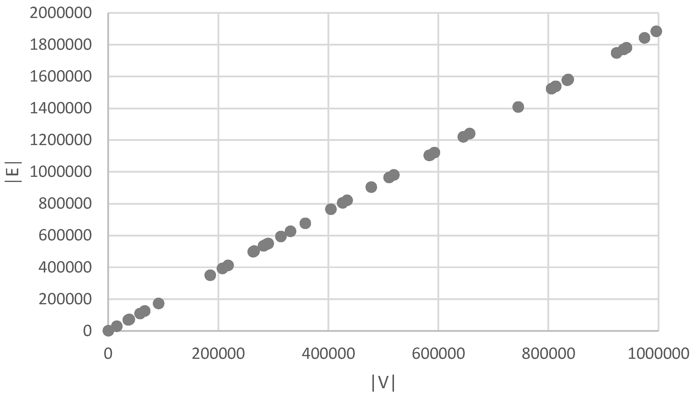
Of course, the exact location where the flat top occurs deserves further investigation. This is done in the following experiment, where we will investigate at what point the maximum number of colors is typically reached. Thus, for a certain number of vertices $\left|V\right|$, we will identify the number of edges $\left|E\right|$ needed in a random Barabási–Albert graph to reach the number of $\left|V\right|$ colors. As we are dealing with stochastic processes, we need to formulate this in a more formal way using confidence intervals. Formally, we will look for the number of edges needed, in order to obtain a $99\%$ chance that we need at least $99\%\ast \left|V\right|$ colors. We can rephrase this: for a graph with $\left|V\right|$ vertices, we need to find the number of edges $\left|E\right|$ such that, if we generate a random Barabási–Albert graph with $\left|V\right|$ vertices and $\left|E\right|$ edges, we have $99\%$ probability that the number of colors needed in the minimal regular equivalence coloring of that graph is at least $99\%\ast \left|V\right|$.

In order to compute meaningful results, a large number of experiments was performed using the algorithm below. The procedure accepts a number of vertices $\left|V\right|$ and calculates the number of edges $\left|E\right|$ that is required to guarantee a $99\%$ chance upon the required use of at least $99\%\ast \left|V\right|$ colors in the minimal regular coloring.

Algorithm 2 Relation between $\left|V\right|$ & $\left|E\right|$ to have many colors

Input:$\left|V\right|$ Output:$\left|E\right|$ 1:  $\left|E\right|\leftarrow \left|V\right|$ 2:  $intervalSize\leftarrow \left|V\right|$ 3:  while $intervalSize>0.01\ast \left|V\right|$ 4:      $passed\leftarrow 0$ 5:      for 1 to 100 do 6:          $G\leftarrow RandomBarabasiAlbert\left(\right|V|,|E\left|\right)$ 7:          $colorsRequired\leftarrow calcColors\left(G\right)$ 8:          if $colorsRequired\ge 99\%\ast \left|V\right|$ then 9:              $passed\leftarrow passed+1$ 10:         end if 11:     end for 12:     if $passed<99$ then 13:         $\left|E\right|\leftarrow \left|E\right|+intervalSize$ 14:     else 15:         $\left|E\right|\leftarrow \left|E\right|-intervalSize$ 16:     end if 17:     $intervalSize\leftarrow intervalSize/2$ 18:  end while 19:  return $\left|E\right|$

In practice, the method has been parametrized by the number of experiments and the confidence-probability, and it moreover contains some shortcuts and optimizations for speed.

Using this algorithm allows us to accurately estimate the relation between $\left|V\right|$ and $\left|E\right|$ to have a $99\%$ chance upon a coloring with more than $99\%\ast \left|V\right|$ colors. The algorithm has been executed 50 times, for various numbers of vertices up to ${10}^6$. Results are shown in Figure 5.

Strikingly, we obtain that the relation is linear, and careful investigation of the data reveals that the slope of the graph $\left|E\right|=s\left|V\right|$ corresponds to about $s\approx 1.89$.

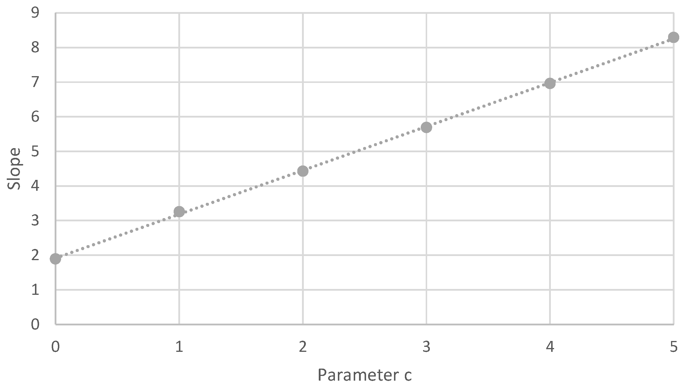
The above results were, as already mentioned, obtained using a Barabási–Albert procedure that always generates random scale-free networks with scaling exponent $\alpha =3$ (see Appendix A). However, these results can be generalized for other scaling exponents, through the use of the parameter c that is used in the Generalized Barabási–Albert generator. This parameter c is related to the scaling exponent $\alpha$ through the equation $\alpha =2+\frac{1}{1+2c}$ and can be used to let $\alpha$ range between 2 and 3 for the resulting generated network.

Using different values for c with $0\le c\le 5$, a number of experiments were run with corresponding values for $\alpha$ such that $2.09<\alpha \le 3$. Most notably, the slope of the graph depicting the relation between $\left|V\right|$ and $\left|E\right|$ (when $99\%$ of the colors is reached, cf. Figure 5) was recalculated for these different values of c and is plotted in Figure 6. Clearly, for $c=0$, we obtain again the slope of Figure 5 itself, which was $s\approx 1.89$. For larger values of c, the value of the corresponding slope grows linearly. These results are striking and puzzling at first sight. However, they can be intuitively understood as follows (using the Barabási–Albert algorithm from Appendix A).

Both for $c=0$ and $c>0$, “Step 2 edges” are added to connect the new vertex to already existing vertices in the network growth process (see Step 2 in Appendix A). Moreover for $c>0$, another $c\ast m$ “Step 3 edges” are added to vertices that are already present in the network (see Step 3 in Appendix A). As these Step 3 edges are added proportionally to the product of the degrees of the vertices involved, they have a strong tendency to confirm the already existing vertex degree structures. Hence, if two vertices have similar roles in the growing network, this similarity tends to be more or less preserved while adding these $c\ast m$ Step 3 edges (despite some random noise effects). This preservation effect is stronger for a Step 3 edge being added than for a Step 2 edge: in the latter case, only the degree weight of one vertex is taken into account, not the degree weight of the new vertex (all new vertices start with the same weight). Looking closely to Figure 6, we can derive from the slope of the graph that adding a single Step 3 edge has approximately the same disruptive effect as adding $0.67$ Step 2 edges.

4.2.2. Real-Life Social Networks

The previous section contained experiments on the behavior of randomly generated networks w.r.t. regular equivalence. We now look at regular equivalence for real-life social networks. To that aim, we downloaded some large networks from the Stanford SNAP data collection [40], which is maintained for the Stanford Network Analysis Project. It is a collection of more than 50 large network datasets with sizes up to tens of millions of vertices and edges. Social networks, web graphs, road networks, internet networks, citation networks, collaboration networks, and communication networks are all represented. We downloaded the following networks for use in our experiments, in order of increasing number of vertices.

• CA-AstroPh: This graph represents a collaboration network on astrophysics obtained from arXiv. It covers scientific collaborations between authors that submitted papers within the Astrophysics category. If two authors u and v co-authored a paper, the graph will contain an (undirected) edge $\{u,v\}$. It will thus contain a small complete subgraph for every paper in the database, as all authors on a single paper always induce a complete graph for these authors.
• CA-CondMat: This dataset corresponds to the collaboration network obtained from arXiv within the Condense Matter Physics category. It was derived in a similar way as the CA-AstroPh network. It has about $23\%$ more vertices than CA-AstroPh but only about half the number of edges.
• Email-Enron: This is an email-communication network, covering email communication within the company Enron, and consisting of about half a million emails. It was disclosed to the public by the Federal Energy Regulatory Commission during the investigation into the Enron scandal in 2001. Vertices represent email-addresses, and an undirected edge $\{u,v\}$ is added to the graph if either u or v sent at least one email to v or u, respectively. Thus, the original direction of communication is not available in the dataset.
• Slashdot0811: This dataset represents a social network derived from the website Slashdot, which is a news website focusing on technology-related subjects. Users can post messages and tag each other as friend or foe. They are represented by vertices and the tags are represented as undirected edges. No distinction is made between friend-tags and foe-tags, so an edge $\{u,v\}$ can have four different meanings. This explains the reduction in $\left|E\right|$ compared to the original dataset.
• DBLP: The DBLP-dataset is derived from the DBLP-database maintained by the University of Trier, which contains a computer science bibliography with a comprehensive list of academic research papers in different subjects all related to computer science. The dataset represents a collaboration network where two authors (vertices) are connected through an (undirected) edge if and only if they co-authored at least one paper.
• LiveJournal: This dataset was derived from LiveJournal, a website community allowing free blogs. People can befriend each other and form groups together. We consider being friends/foes a symmetric relation, and represent users as vertices and their friendships as undirected edges.

The networks were processed in order to prepare them for analysis by our software. This involved, among other things, ensuring edges are undirected, removing double edges, and checking for inconsistencies. The resulting networks that were used for the rest of the analysis are listed in

Table 1. Real-life social networks.

Network	|V|	|E|	|E|/|V|
CA-AstroPh	18,772	198,050	10.6
CA-CondMat	23,133	93,439	4.0
Email-Enron	36,692	183,831	5.0
Slashdot0811	77,360	469,180	6.1
DBLP	317,080	1,049,866	3.3
LiveJournal	3,997,962	34,681,189	8.7

.

After calculation of the actual number of colors required in the minimal regular coloring of these real-life social networks, it was obtained that they required only a relatively small fraction of colors. Results are shown in

Table 2. Results for real-life social networks.

Network	|C|	|C|/|V|	Runtime (s)
CA-AstroPh	14,734	$78\%$	0.9
CA-CondMat	17,131	$74\%$	0.5
Email-Enron	20,417	$56\%$	0.4
Slashdot0811	61,457	$79\%$	1.4
DBLP	233,466	$74\%$	14.5
LiveJournal	3,703,526	$93\%$	1684

. In this table, we will denote the number of colors used in the minimal regular coloring as $\left|C\right|$. As can be seen in the column $\left|C\right|/\left|V\right|$, the percentage of colors used ranges from $56\%$ to $93\%$, while the minimal coloring was typically calculated very fast, matching the results from Figure 2.

It is striking that 4 out of 6 real-life complex social networks have about the same ratio $\left|C\right|/\left|V\right|$, around $76\%$. In contrast, the two other networks investigated have either a much lower ($56\%$) or much higher ($93\%$) ratio. Additionally, the runtime for processing the LiveJournal dataset seems to be higher than expected on the basis of its size alone. The underlying social phenomena and/or topological structures that give rise to these wildly differing values is not clear and should be further investigated.

5. Discussion

In this work, we investigated social networks using regular equivalences. Minimal regular equivalence was introduced, which allows one to attach roles to vertices with a similar local neighborhood-structure, and which keeps a very good balance between being too strict and too loose for efficient analysis of the global network structure. The hierarchic position of minimal regular equivalence with respect to other equivalence relations was proven, and a fast and efficient algorithm was introduced. Six real-life social networks with up to $4\times {10}^6$ vertices and $35\times {10}^6$ edges were investigated, next to networks obtained with a Barabási–Albert random network generator. It was obtained that, for a certain value of the scaling exponent $\alpha$, the ratio of the number of edges to the number of vertices is directly related to the minimum number of regular colors needed. The tipping point, where almost all possible colors are needed, is reached at a certain ratio which is constant for all networks with the same scaling exponent $\alpha$. Moreover, this ratio was demonstrated to have a linear relation to the parameter c that is used in the generalized Barabási–Albert generator, and an intuitive explanation for this effect was given. Because regular equivalence as defined in this paper is a fast and useful method to structurally analyze networks, it can also be used to test whether network-generators mimic these equivalences well.

Future Work

First of all, it is of prime importance to apply the approach to many more real-life social networks, and to investigate the underlying social phenomena that are the reasons for the different values for $\left|C\right|/\left|V\right|$. What are the structures of the classes found? Are they homogeneous across the network? How different are they from other (regular) equivalences? If we want to calculate the regular equivalence relation for really large networks with up to ${10}^9$ vertices, we might need to scale up the approach taken, which can be done through improving the algorithm even further via incremental updates of spectra instead of a double loop, which will decrease the computational complexity. By then, it will be possible to compare the number of colors needed for real networks with their generated counterparts and investigate any potential significant discrepancies. We expect these mismatches to occur for at least certain types of real-life networks, and as such network generators should be redesigned so their output mimics the regular equivalence structure in a more accurate way. Interesting future work can thus include a thorough study of different types of real-life networks with respect to regular equivalence as defined in this paper and the design of new network generators whose output features the same regular equivalence structure as real-life networks. Lastly, the entire approach should be adapted to directed networks. This involves an appropriate definition for directed regular equivalence, and accompanying algorithms for both calculating the directed colorings and generating random directed networks with matching colorings.

References

- Erdos, P.; Rényi, A. On random graphs. Publ. Math. Debr. 1959, 6, 290–297. [Google Scholar]
- van Steen, M. Graph Theory and Complex Networks: An Introduction; On Demand Publishing, LLC-Create Space: North Charleston, SC, USA, 2010. [Google Scholar]
- Watts, D.J.; Strogatz, S.H. Collective dynamics of’small-world’networks. Nature 1998, 393, 440–442. [Google Scholar] [CrossRef] [PubMed]
- Csermely, P. Weak Links: The Universal Key to the Stability of Networks and Complex Systems; Springer-Verlag: Berlin/Heidelberg, Germany, 2006. [Google Scholar]
- Barabási, A.; Ravasz, E.; Vicsek, T. Deterministic scale-free networks. Physica A 2001, 299, 559–564. [Google Scholar] [CrossRef] [Green Version]
- Albert, R.; Barabasi, A.L. Statistical mechanics of complex networks. Rev. Mod. Phys. 2002, 74, 47–97. [Google Scholar] [CrossRef] [Green Version]
- Barabási, A.L. Linked: The New Science Of Networks; Perseus Books Group: New York, NY, USA, 2002. [Google Scholar]
- Barabási, A.L.; Albert, R. Emergence of Scaling in Random Networks. Science 1999, 286, 509–512. [Google Scholar] [Green Version]
- Dorogovtsev, S.N.; Mendes, J.F.F. Evolution of Networks; Oxford University Press, Inc.: New York, NY, USA, 2003. [Google Scholar]
- Vega-Redondo, F. Complex Social Networks; Cambridge University Press: Cambridge, UK, 2007. [Google Scholar]
- Dorogovtsev, S.N.; Mendes, J.F.F.; Samukhin, A.N. Structure of Growing Networks with Preferential Linking. Phys. Rev. Lett. 2000, 85, 4633–4636. [Google Scholar] [CrossRef] [Green Version]
- Holme, P.; Kim, B.J. Growing scale-free networks with tunable clustering. Phys. Rev. E 2002, 65, 026107. [Google Scholar] [CrossRef] [Green Version]
- Chen, Q.; Shi, D. The modeling of scale-free networks. Physica A 2004, 335, 240–248. [Google Scholar] [CrossRef]
- Wasserman, S.; Faust, K. Social Network Analysis; Cambridge University Press: Cambridge, UK, 1995. [Google Scholar]
- Easley, D.; Kleinberg, J. Networks, Crowds, and Markets; Cambridge University Press: New York, NY, USA, 2010. [Google Scholar]
- Lorrain, F.; White, H.C. Structural equivalence of individuals in social networks. J. Math. Soc. 1971, 1, 49–80. [Google Scholar] [CrossRef]
- Hanneman, R.; Riddle, M. Introduction to Social Network Methods; University of California: Oakland, CA, USA, 2005. [Google Scholar]
- Newman, M. Networks: An Introduction; OUP Oxford: Oxford, UK, 2010. [Google Scholar]
- Borgatti, S.P.; Everett, M.G. Notions of Position in Social Network Analysis. Sociol. Methodol. 1992, 22, 1–35. [Google Scholar] [CrossRef]
- Jin, R.; Lee, V.E.; Li, L. Scalable and Axiomatic Ranking of Network Role Similarity. ACM Trans. Knowl. Discov. Data 2014, 8, 3:1–3:37. [Google Scholar] [CrossRef]
- Fan, T.F.; Liau, C.J. Logical characterizations of regular equivalence. Artif. Intell. 2014, 214, 66–88. [Google Scholar] [CrossRef]
- Marx, M.; Masuch, M. Regular equivalence and dynamic logic. Soc. Netw. 2003, 25, 51–65. [Google Scholar] [CrossRef] [Green Version]
- Brandes, U.; Lerner, J. Structural Similarity: Spectral Methods for Relaxed Blockmodeling. J. Class 2010, 27, 279–306. [Google Scholar] [CrossRef] [Green Version]
- Boyd, J.P.; Jonas, K.J. Are social equivalences ever regular?: Permutation and exact tests. Soc. Netw. 2001, 23, 87–123. [Google Scholar] [CrossRef]
- Casse, J.I.; Shelton, C.R.; Hanneman, R.A. A new criterion function for exploratory blockmodeling for structural and regular equivalence. Soc. Netw. 2013, 35, 31–50. [Google Scholar] [CrossRef]
- Prota, L.; Doreian, P. Finding roles in sparse economic hierarchies: Going beyond regular equivalence. Soc. Netw. 2016, 45, 1–17. [Google Scholar] [CrossRef]
- Barrière, L.; Comellas, F.; Dalfó, C.; Fiol, M.A. Deterministic hierarchical networks. Physica A 2016, 49. [Google Scholar] [CrossRef]
- Fan, T.F.; Liau, C.J.; Lin, T.Y. A theoretical investigation of regular equivalences for fuzzy graphs. Int. J. Approx. Reason. 2008, 49, 678–688. [Google Scholar] [CrossRef] [Green Version]
- Doran, D. On the discovery of social roles in large scale social systems. Soc. Netw. Anal. Min. 2015, 5, 1–18. [Google Scholar] [CrossRef]
- Henderson, K.; Gallagher, B.; Eliassi-Rad, T.; Tong, H.; Basu, S.; Akoglu, L.; Koutra, D.; Faloutsos, C.; Li, L. RolX: Structural Role Extraction and Mining in Large Graphs. In Proceedings of the 18th ACM SIGKDD International Conference on Knowledge Discovery and Data Mining, KDD 2012, Beijing, China, 12–16 August 2012. [Google Scholar]
- Vega, D.; Magnani, M.; Montesi, D.; Meseguer, R.; Freitag, F. A new approach to role and position detection in networks. Soc. Netw. Anal. Min. 2016, 6, 1–23. [Google Scholar] [CrossRef]
- Vega, D.; Meseguer, R.; Freitag, F.; Magnani, M. Role and Position Detection in Networks: Reloaded. In Proceedings of the 2015 IEEE/ACM International Conference on Advances in Social Networks Analysis and Mining (ASONAM), Paris, France, 25–28 August 2015. [Google Scholar]
- Rossi, R.A.; Ahmed, N.K. Role Discovery in Networks. IEEE Trans. Knowl. Data Eng. 2015, 27, 1112–1131. [Google Scholar] [CrossRef] [Green Version]
- Purcell, C.; Rombach, P. On the complexity of role colouring planar graphs, trees and cographs. J. Discr. Alg. 2015, 35, 1–8. [Google Scholar] [CrossRef] [Green Version]
- Chen, J.; Saad, Y. Dense Subgraph Extraction with Application to Community Detection. IEEE Trans. Knowl. Data Eng. 2012, 24, 1216–1230. [Google Scholar] [CrossRef]
- Borgatti, S.; Everett, M. Two algorithms for computing regular equivalence. Soc. Netw. 1993, 15, 361–376. [Google Scholar] [CrossRef] [Green Version]
- Newman, M.E.J. Fast algorithm for detecting community structure in networks. Phys. Rev. E 2004, 69, 066133. [Google Scholar] [CrossRef] [Green Version]
- Boyd, J.P. Finding and testing regular equivalence. Soc. Netw. 2002, 24, 315–331. [Google Scholar] [CrossRef]
- Sedgewick, R.; Wayne, K. Algorithms; Pearson Education: London, UK, 2011. [Google Scholar]
- Leskovec, J.; Krevl, A. SNAP Datasets: Stanford Large Network Dataset Collection. Available online: http://snap.stanford.edu/data (accessed on 30 November 2018).
Figure 1.
Vertices u and v are regularly equivalent, but not automorphically.