Predicting the Aqueductal Cerebrospinal Fluid Pulse: A Statistical Approach


1
Institute for Sport, Physical Activity and Leisure, Leeds Beckett University, Leeds LS6 3QT, UK
2
Medical Biophysics Laboratory, University of Bradford, Bradford BD7 1DP, UK
3
IRCCS Fondazione Don Carlo Gnocchi ONLUS, 20148 Milan, Italy
*
Author to whom correspondence should be addressed.
Appl. Sci. 2019, 9(10), 2131; https://doi.org/10.3390/app9102131
Submission received: 31 March 2019
/
Revised: 9 May 2019
/
Accepted: 22 May 2019
/
Published: 24 May 2019
(This article belongs to the Section Applied Biosciences and Bioengineering)
Abstract
:The cerebrospinal fluid (CSF) pulse in the Aqueduct of Sylvius (aCSF pulse) is often used to evaluate structural changes in the brain. Here we present a novel application of the general linear model (GLM) to predict the motion of the aCSF pulse. MR venography was performed on 13 healthy adults (9 female and 4 males—mean age = 33.2 years). Flow data was acquired from the arterial, venous and CSF vessels in the neck (C2/C3 level) and from the AoS. Regression analysis was undertaken to predict the motion of the aCSF pulse using the cervical flow rates as predictor variables. The relative contribution of these variables to predicting aCSF flow rate was assessed using a relative weights method, coupled with an ANOVA. Analysis revealed that the aCSF pulse could be accurately predicted (mean (SD) adjusted r2 = 0.794 (0.184)) using the GLM (p < 0.01). Venous flow rate in the neck was the strongest predictor of aCSF pulse (p = 0.001). In healthy individuals, the motion of the aCSF pulse can be predicted using the GLM. This indicates that the intracranial fluidic system has broadly linear characteristics. Venous flow in the neck is the strongest predictor of the aCSF pulse.
1. Introduction
The cerebrospinal fluid (CSF) pulse in the Aqueduct of Sylvius (AoS) (the aqueductal CSF (aCSF) pulse) is closely linked with the motion of the lateral ventricles [1] and can be used as a surrogate measure of brain tissue ‘stiffness’ [2]. As such, the aCSF pulse is often measured in order to evaluate structural changes that may occur in the brain parenchyma. Numerous studies have found increased pulsatility of the aCSF to be associated with multiple sclerosis (MS) [3,4,5,6,7], normal pressure hydrocephalus (NPH) [8,9,10,11,12,13], and white matter (WM) alterations [14,15], suggesting that increases in the amplitude of the aqueductal pulse may be linked to pathological changes.
It has been shown that the dynamics of the aCSF pulse are influenced by the patency of the cerebral venous drainage vessels [16], with compression of the internal jugular veins (IJVs) leading to: (i) accumulation of blood in the cortical veins [17]; (ii) increased brain tissue ‘stiffness’ [2]; and increased aCSF pulse amplitude [2]. As such, a relationship exists between the intracranial fluid dynamics and blood flow in the neck. This is because the cranium is a rigid container and the parenchymal tissue and fluids enclosed within it are incompressible [18]. Consequently, it is possible to characterize the behaviour of the various intracranial fluids by interpreting fluid flow signals acquired from the arterial, venous and CSF vessels in the neck [19,20,21,22]. Given this, we hypothesized that it should be possible to predict aCSF motion from the extracranial arterial, venous and CSF flow rate signals. Therefore, we designed the ‘proof-of-concept’ pilot study presented here, in which we used the general linear model (GLM) to predict the motion of the aCSF pulse. The primary aim of the study was to test whether or not a statistical linear model could accurately predict the motion of the aCSF pulse using only data acquired from the vessels in the neck. As a secondary aim, we also wanted to identify the cervical flow signals (i.e., arterial, venous or CSF) that best predicted the motion of the aCSF, as this might assist in better understanding the factors that influence the motion of the CSF in the AoS. As such, we hoped to gain new insights into the physiology of the intracranial fluidic system in healthy individuals. Furthermore, we anticipated that the model might be a useful tool for identifying changes in the dynamics of the intracranial fluidic system that could be of clinical importance.
2. Materials and Methods
2.1. Subjects
Thirteen healthy adults were enrolled in the study. Because the prevalence of diseases such as Alzheimer’s disease and vascular dementia, which are associated with brain atrophy [23], greatly increases over the age of 65 years [24], inclusion criteria were age <65 years and a normal neurological examination. Exclusion criteria were: history of neurological, cardiovascular or metabolic disorders and abnormalities on brain anatomical MRI.
The study was approved by the local Ethics Committee of Don Gnocchi Foundation (Milan, Italy) and a written informed consent was obtained from all subjects prior to study entry.
2.2. Magnetic Resonance Acquisition and Processing
Brain and neck MRI were acquired from all subjects, using a 1.5 Tesla scanner (Siemens Magnetom Avanto, Erlangen, Germany), equipped with an 8-channel head coil and a 4-channel neck coil. The acquisition protocol consisted of brain anatomical scan and neck vein morphological and hemodynamic sequences. First, brain and neck T1-weighted localizer, were acquired for the slice positioning of the subsequent sequences. Then, brain 2D dual-echo turbo spin echo allowed us to assess any anatomical abnormalities (TR = 2,650 ms, TE = 28/113 ms, echo train length = 5, flip angle = 150°, 50 interleaved, 2.5-mm-thick axial slices with a matrix size = 256 × 256, interpolated to 512 × 512, FOV = 250 × 250 mm). The neck vein morphology was assessed using a 2D time-of-flight (TOF) MR venography of the neck, with a saturation band positioned caudal to the 128 axial slices (in-plane resolution = 0.5 × 0.5 mm2, slice thickness = 3 mm, distance factor between subsequent slices = −20, FOV = 256 × 192 mm2, TR = 26 ms, TE = 7.2 ms, flip angle = 70°). Maximum intensity projection (MIP) was performed for the visualization of the veins with sagittal and coronal views. The MIPs allowed us to position the following sequence and to evaluate the morphology of the IJV and secondary drainage routes. Finally, arterial and venous flows through the main cervical vessels, CSF flow between the second and the third cervical vertebrae (C2/C3 level) (cCSF) and aCSF were assessed using three retrospective cardiac gated 2D PC MRI. The sequence parameters were respectively (blood/cCSF/aCSF): TR = 33.75/30.2/30.2 ms, TE = 5.11/7.6/7.6 ms, flip angle = 30°/10°/10°, matrix size = 288 × 384/256 × 256/256 × 256, pixel size = 0.67 × 0.67/0.62 × 0.62/0.45 × 0.45 mm2, slice thickness = 4/4.5/4.5 mm, and maximum encoding velocity Venc 60//15/15 cm/s. A finger pulse oximeter was used in order to reconstruct different time points in the cardiac cycle (CC), depending on the heart rate frequency. The slice of the PC sequences were positioned perpendicularly to the flow of interest: for the cervical blood flow, the sagittal neck localizer (Figure 1A) and the sagittal and coronal TOF MIP on the images (Figure 1B,C) were used for positioning the PC slice at the C2/C3 level perpendicularly to the IJVs (Figure 1A,B,C); for the cCSF flow the sagittal neck localizer was used for positioning perpendicularly to the spinal canal at C2/C3 level (Figure 1A); for the aCSF flow the sagittal T1-weighted brain localizer was used (Figure 1D) for positioning perpendicularly to the AoS.
The flow data were processed with FlowQ software, an in-house program written in MATLAB (The Mathworks, Natick, MA, USA), with the methods described in [25] by a single trained examiner. Briefly, for every PC sequence, the processing consisted in manually drawing two kinds of regions of interest (ROIs) on the magnitude and phase images. The first one was placed in the structures of interest for their flow quantification, and the second one consisted of at least three ROIs in stationary structures near to the structure of interest, for the estimation and removal of the phase offset. The IJVs, vertebral veins (VVs), deep cervical veins (DCVs), internal carotid arteries, and vertebral arteries were segmented on the PC images with Venc = 60 cm/s (Figure 2A,B)). The contours were drawn in the first time point and copied for every time point in the CC, manually adjusting them if needed. When we visually detected a ROI that was affected by phase aliasing, pixel phase values were corrected with the algorithm described in a previous work [26]. Briefly, the FlowQ software performs phase unwrapping evaluating the phase value inside the vessel during the whole CC, detecting the phase values lower/greater than 0.3π/−0.3π, for pixels inside an artery/vein respectively, and then increasing/decreasing them by 2π.
The cCSF (Figure 2C,D) and the aCSF (Figure 2E,F) were segmented on the PC images with Venc = 15cm/s. The CSF contours were drawn on the phase image corresponding to the time point with the highest caudal flow velocity (Figure 2D,F), as this shows the highest contrast. The magnitude image (Figure 2C,E)) was used to increase the confidence of the contours. For every pixel inside the segmented vessels or the CSF, and for every time point, the phase value was corrected by the offset subtracting the average phase of the stationary tissue ROIs, then it was corrected by the aliasing, and finally it was mapped to velocity. According to Siemens convention, positive CSF flow corresponds to the cranial direction, negative CSF flow corresponds to the caudal direction. The flow rate (in ml/s) was computed for each time point, based on the mean velocity and the cross sectional area of the corresponding structure.
2.3. Flow Data Analysis
Flow data and statistical analysis were undertaken using in-house algorithms written in Matlab (Mathworks, Natick, Mass) and R (R Core Team (2013). R: A language and environment for statistical computing. R Foundation for Statistical Computing, Vienna, Austria). Arterial flow rate was computed as the sum of the flow in the internal carotid and vertebral arteries and the venous flow rate as the sum of the IJV, VV, and DCV flow rates. The arterial, venous, cCSF and aCSF flow rate signals were resampled to 32 data points over the CC (Figure 2G,H). For each fluid, the flow rate caudal and cranial peak amplitudes were computed. The pulsatility index (PI) and the resistance index (RI) [27] were calculated as the difference between systolic and diastolic peaks normalized by the mean or the systolic peak flow rate, respectively. For the CSF, we computed a caudal and a cranial RI, normalizing by the systolic or diastolic peak, respectively. The cCSF and aCSF stroke volumes (i.e., the average CSF volume displaced throughout the CC) were calculated by averaging the absolute positive and negative flow rate integrals [28]. The arteriovenous delay (AVD) between the peaks in the arterial and inverted venous flow rate signals was also computed [29,30].
2.4. Statistical Analysis
The mean and median values across the subjects were computed for all the continuous variables. For each subject the Pearson correlations between the arterial, venous, cCSF and aCSF flow rates were calculated and the mean and SD of the respective r-values computed. Correlations (r values) of 0.30–0.49 (r2 = 0.09–0.24) were considered weak, 0.50–0.69 (r2 = 0.25–0.48) were moderate, 0.70–0.89 (r2 = 0.49–0.80) were strong and higher than 0.90 (r2 = 0.81) was very strong.
For each subject, multiple linear regression analysis was undertaken using the GLM to evaluate the extent to which the cervical arterial, venous and cCSF flow rate signals (predictor variables) could be used to predict the aCSF signal (response variable). The relative contribution of the predictor variables in predicting the aCSF flow rate was assessed using the relative weights method described by Johnson [31,32] (see Appendix A for further explanation). This involved creating a series of orthogonal counterparts of the original predictors and applying singular value decomposition to identify the relative importance of the predictor variables with respect to aCSF. The resulting relative weights for the predictor variables were then evaluated using a one-way ANOVA with post-hoc pairwise t-tests, which were Holm corrected for multiple comparisons [33]. Differences between the fit (adjusted r2 value) achieved by the GLM in the male and female subjects was assessed using an independent two-tailed t-test. For all tests, p values <0.05 were deemed to be significant.
3. Results
3.1. Demographic Results
The 13 subjects included in this study were 9 female and 4 males, average age 33.2 years old (SD = 10.6 years; range 20–60 years). Demographics are shown in Table 1.
3.2. Magnetic Resonance Imaging Results
The average and SD (across subjects) of the arterial, venous, cCSF, and aCSF flow rate curves are shown in Figure 3. The mean value and SD of their peaks, average value, and PI are reported in Table 2. The pulsatility of the cervical venous flow rate (range –8.89 to −15.71 mL/s; mean (SD) PI = 0.56 (0.23); mean (SD) RI = 0.43 (0.14)) was less (p < 0.001) than that of the arterial flow rate (range 8.36 to 19.59 mL/s; PI mean (SD) = 0.906 (0.224); mean (SD) RI = 0.57 (0.07)), with the cCSF flow fluctuating (range –2.70 to 1.72 mL/s; mean (SD) caudal RI = −1.65 (0.12); cranial RI = 2.58 (0.28)) around a mean flow rate close to zero. The amplitude of the aCSF pulse (range: –0.10 to 0.09 mL/s; mean (SD) caudal RI = −1.95 (0.26); cranial RI = 2.14 (0.34)) was an order of magnitude smaller than the cCSF pulse, with the mean stroke volume of the two being 24.10 (SD = 14.50) µL/beat and 530.80 (SD = 208.00) µL/beat (Table 1), respectively. The mean AVD was 87.67 (SD = 78.78) ms (Table 1).
3.3. Data Analysis Results
The results of the correlation analysis, which are presented in Table 3, reveal a strong negative correlation (mean (SD) r = −0.837 (0.126)) between the arterial and cCSF flow rates over the CC. Conversely; a strong positive correlation (mean (SD) r = 0.763 (0.266)) was observed between the venous and aCSF flows. Moderate correlations were also found between the venous and cCSF (mean (SD) r = 0.621 (0.178)), and venous and arterial (mean (SD) r = −0.601 (0.293)) flow rates, while the remaining correlations were weaker.
Multiple linear regression analysis (Table 4) revealed that it was possible with a high degree of accuracy (mean (SD) adjusted r2 = 0.794 (0.184)) to predict the aCSF flow rate signal using the arterial, venous and cCSF signals as predictors (p < 0.001 for all models except that for subject 5031 which was p = 0.004). Partial adjusted r2 values were: arterial (mean r2 = 0.342 (SD = 0.278)); venous (mean r2 = 0.641 (SD = 0.260)); and cCSF (mean r2 = 0.408 (SD = 0.264)). However, no correlation was observed between AVD values and the model adjusted r2 values (r = −0.041; p = 0.893). No significant difference (p = 0.658) was observed between the adjusted r2 values for the male (mean (SD) adjusted r2 = 0.830 (0.165)) and female (mean (SD) adjusted r2 = 0.778 (0.198)) subjects.
The relative importance weights of the aCSF signal predictor variables are presented in Table 4. These reveal that the venous flow rate was the strongest predictor (F = 7.86 (df = 2 & 36), p = 0.001). Post-hoc t-tests subsequently revealed that the relative weight of the venous flow rate (48.886 ± 20.415) was significantly higher compared to that of the arterial (20.721 ± 22.027, p = 0.001) and cCSF signals (30.393 ± 10.705, p = 0.030).
4. Discussion
The principal finding of the study is that the motion of the aCSF pulse can be accurately predicted using the arterial, venous and cCSF flow rates in the neck and a simple linear regression model (i.e., GLM). An exemplificative typical subject (subject 5005) is shown in Figure 1 and Figure 2, where the arterial, venous, cCSF (Figure 2G), aCSF (Figure 2H) and predicted aCSF (Figure 2H) flow rate curves are shown. The venous morphology is also shown, with the subject’s coronal TOF MIP (Figure 1C), where the symmetric IJVs are well visible. Given that the cranium is a rigid container filled with incompressible gels (i.e., the brain parenchyma) [18] and fluids (i.e., blood, CSF and interstitial fluid), it is perhaps not unexpected that the craniospinal fluid system should behave in a linear manner. Like all hydraulic systems involving rigid vessels and incompressible fluids, one would expect expansion in one fluid component within the system to have an instantaneous effect on the other fluid components in the system. Therefore, it is to be expected that motion of the aCSF will be influenced by the characteristics of the fluids entering and leaving the cranium via the neck. Indeed, it has been shown that the volumetric changes in the various fluid compartments of the intracranial space can be computed using fluid flow rates in the vessels of the neck [20]. As such, our finding that the GLM can be used to predict aCSF appears to support the opinion that the intracranial fluidic system behaves in a broadly linear manner.
In our study, we found that the median adjusted r2 value for the model was 0.857. This implies that, on average, approximately 86% of the variance in the aCSF pulse could be explained by the cervical arterial, venous and cCSF flow rates. While this demonstrates that the behaviour of the system is broadly linear, it is noticeable that about 14% of the variance in the cCSF remained unexplained, suggesting that other, possibly non-linear, factors may influence the dynamics of the cCSF pulse. Chief amongst these is the presence of compliance in the system, as indicated by the presence of an AVD between the arterial blood entering the cranium and the venous blood leaving it (Table 1), which in healthy adults has been reported as 89 ± 40 ms [29], very similar to the value of 87.7 ± 78.8 ms observed in our study (p = 0.97). Although intracranial compliance is not fully understood, it is thought that it is strongly influenced by compliance in the spinal column [34] and also by the characteristics of the cerebral venous drainage system [12,35,36,37]. Although the cranium contains incompressible fluids and gels, it is not a closed system, because venous blood can freely exit the cranium via the IJVs and VVs—something that imparts a functional compliance to the whole system. However, if the venous drainage pathways become constricted, then blood will tend to accumulate in the cerebral veins [17] causing the brain parenchyma to become stiffer [2] and intracranial compliance to decrease. Given also that constricted IJVs have been associated with increased aCSF pulsatility [2], it is perhaps not surprising that the variable importance analysis (Table 4) found the cervical venous flow rate signal to be the best predictor of the aCSF pulse. As such, this supports the findings of Lagana et al. [20] who observed that the motion of the aCSF pulse was strongly correlated with accumulation of venous blood in the cranium. It also reinforces the opinion [12,38] that the cerebral veins play an important role in the regulation of the dynamic intracranial equilibrium.
While most of the subjects in our study exhibited similar characteristics with regard to the performance of the linear model, it is noticeable that for a couple of individuals (subjects 5010 and 5031) the explained variance (i.e., the adjusted r2 value) was much lower than the median adjusted r2 value for the whole study cohort. For example, with subject 5031 the GLM was only able to explain 29.5% of the variance in the aCSF pulse, which was much less than that explained in the other subjects. If we compare subject 5031 (a 21 year old female—Figure 4) with a typical individual such as subject 5005 (a 38 year old male—Figure 2), for whom the model explained 88.4% of the variance, it can be seen that the arterial systolic peak was much greater in subject 5031 than in subject 5005. Also the venous flow rate profile in subject 5031 was atypical, with the venous diastolic ‘peak’ (i.e., the minimum value in the inverted venous signal shown in Figure 2G and Figure 4A) occurring much earlier in the CC in subject 5031 compared with subject 5005. Furthermore, subject 5031 exhibited a somewhat atypical aCSF flow rate profile (Figure 4B) compared with subject 5005 (Figure 2H), who was more representative of the study cohort. Having said this, both subjects exhibited venous morphologies that appeared normal (Figure 1B,C; and Figure 4C). Noticeably however, the AVD for subject 5031 was 151.6 ms, while it was only 89.9 ms for subject 5005, indicating that intracranial compliance was much greater in the former compared with the latter. While the increase in intracranial compliance provides a plausible explanation for the poor prediction performance of the model in subject 5031, it should be noted that we found no correlation between AVD and model adjusted r2 value in the study cohort as a whole. Therefore, we cannot be certain that the observed model performance in subject 5031 is directly attributable to the increase in the AVD as other unobserved factors might be at work.
Interestingly, while for most subjects the cervical venous flow rate signal was the best predictor of aCSF pulse, for subjects 5010 and 5031 (the two subjects with the lowest adjusted r2 values) it was the cCSF signal that was the dominant predictor (Table 4). As such, this suggests that venous anomalies might have contributed to the lower r2 values observed for these subjects. Indeed, subject 5010 was found to have turbulent and low flow in the left IJV (Figure 5A), as well as a particularly high aCSF stroke volume of 51 µL/beat (Table 1). By contrast, no morphological venous abnormalities were observed in subject 5031 (Figure 4C), although the profile of the venous flow signal in Figure 4A was atypical. While the reasons for this atypical behaviour are unknown, given that 70% of the intracerebral blood volume lies within the veins [39] and that these are thought to play an important role in regulating cerebral compliance [12,35,36,37], it may be that the changes in the dynamics of the cerebral venous drainage system contributed to the low adjusted r2 value in this subject. Intracranial compliance is dependent on the cerebral venous drainage system, which because it is ‘open’ allows fluid to move out of the cranium [36]. This process is however mediated by the interaction between the CSF and the cortical bridging veins in the subarachnoid space, which regulates the accumulation of venous blood in the cranium [20]. If for any reason this mechanism should become impaired, then it has the potential to alter both the dynamics of the intracranial fluidic system and the compliance of the intracranial space. However, while changes in the venous system may have contributed to the observed results for subjects 5010 and 5031, further work will be required to fully explain why the r2 values observed for these subjects were appreciably lower than for the other subjects. Notwithstanding this, it should be noted that the low turbulent flow in the left IJV of subject 5010 would have resulted in a less precise PC MRI flow estimate for this vessel, something that might have contributed to a less accurate prediction of the aCSF pulse in this subject. With regard to this, it is noticeable that for subject 5006, who exhibited extensive collateral veins and posterior veins but no turbulence (Figure 5B), the model adjusted r2 value was 0.894 (Table 4), further suggesting that the presence of turbulent flow might have a detrimental effect on the predictive accuracy of the aCSF model.
The dynamics of the aCSF pulse are an issue of clinical importance. Increased amplitude of the aCSF pulse has been shown to be associated with MS [3,4,5,6,7], NPH [8,9,10,11,12,13], and early-stage WM changes [14,15]. However, the mechanism linking aCSF pulse dynamics with these pathologies is poorly understood. Because the phenomenon has been linked with an increase in the ‘stiffness’ of the brain tissue [2], it may be that increased aCSF stoke volume is a sign that the cerebral windkessel mechanism [40,41,42], which regulates blood flow through the parenchyma, has become impaired [43]. Impairment of the windkessel mechanism has been shown to occur with bilateral compression of the IJVs, resulting in increased pulsation in the pial arteries [44]. This has been linked with WM changes in elderly individuals, with increased pulsatility in the parenchymal vascular bed associated with WM microstructural changes [15], small vessel disease [45] and leukoaraiosis [43]. Increased aCSF stroke volume might also be associated with transependymal seepage of CSF into the parenchyma, reversing the normal direction of flow [46]. Being a semipermeable barrier between the brain parenchyma and the CSF in the ventricles [47] the ependymal wall is vulnerable to disruption [46]. Indeed, in NPH patients the periventricular tissue is characterized by disruption of the ependyma, and by oedema, neuronal degeneration, and ischemia [48]. In patients with communicating hydrocephalus transependymal CSF resorption appears to be associated with caudal-to-cranial net aqueductal flow, whereas the direction is cranial-to-caudal in healthy individuals [12]. Collectively, this highlights the need to better understand the dynamics of the aCSF pulse and its role as an indicator neurological well-being. As such, there is a need for new methodologies, such as the statistical linear model outlined above, which evaluate the aCSF pulse, so that a better understanding can be gained of its behaviour in relation to changes in the cervical arterial, venous and CSF flows.
It should be noted that the present work was intended to be a ‘proof-of-concept’ pilot study designed to test the validity of the statistical linear model presented above. As such the study was subject to a number of limitations. Chief amongst these was the small size of the study cohort. Although we found that the model could predict the motion of the aCSF pulse with a high degree of accuracy (r2 > 0.85) for the most of the healthy subjects in this pilot study, further work, involving a larger cohort, will be required to confirm this finding. Furthermore, because only four male subjects were recruited to the pilot study, it was not possible to undertake any meaningful statistical comparison between the sexes, as this analysis would have been grossly statistically underpowered. Therefore, it is recommended that in future studies sufficient numbers of males and females be recruited in order to make comparisons between the sexes. More work will also be required to evaluate the clinical potential of the linear model. In particular, it is important to understand why certain individuals, such as subject 5031, who otherwise appeared healthy, should behave in such an atypical manner. It may be that in these individuals the model is identifying signs of early-stage structural changes in the intracranial fluid dynamics, which might ultimately lead to a pathology. If this is the case then the model may have considerable potential as a diagnostic tool. Further work is also needed to better understand the intracranial fluid dynamic changes that occur in MS and NPH patients. In both these conditions the amplitude of the aCSF pulse has been shown to markedly increase [4,5,12,13] and it may be that the linear model might be able to shed new insights into the altered fluid dynamics associated with these neurological diseases.
5. Conclusions
In this pilot study we have shown that it is possible in healthy individuals to predict the motion of the aCSF pulse with a high degree of accuracy (median r2 = 0.857) using arterial, venous and CSF flow rate data acquired from vessels in the neck and a simple linear model. This indicates that the intracranial fluidic system behaves in a broadly linear manner. Furthermore, we have been able to show that cervical venous flow rate is the most influential predictor of the aCSF pulse. As such, our findings support those of other researchers [2,16,20], all of whom suggested a biomechanical link between the CSF pulse in the AoS and the cerebral venous drainage system. Notwithstanding this, the study was limited by its small cohort size and therefore further work will be required involving a larger sample size to confirm our findings.
Author Contributions
Conceptualization, C.B., M.L. and S.S.; Methodology, C.B. and M.L.; Software, C.B. and M.L.; Formal Analysis, C.B. and M.L.; Investigation, C.B., P.C., M.L.; Resources, C.B., P.C., M.L.; Data Curation, C.B. and M.L.; Writing—Original Draft Preparation, C.B.; Writing—Review & Editing, C.B., S.S., P.C., M.L; Supervision, C.B.,M.L.; Project Administration, C.B., P.C., M.L.; Funding Acquisition, C.B., P.C., M.L.
Funding
This research received no external funding
Conflicts of Interest
The authors declare no conflict of interest.
Appendix A
Relative weights method. When multiple regression is used for explanatory purposes, it is often the case that investigators are interested in the extent to which each predictor variable contributes to prediction of the response variable. In short, investigators often want to quantify the relative importance of the predictor variables as the proportionate contribution that each makes to the overall r2 value of the model.
In order to draw inference about the relative importance of predictors, researchers often examine the standardized regression coefficients. While this is acceptable when the predictor variables are uncorrelated, this method can be problematic when the predictors are correlated and may lead to erroneous conclusions being drawn. To overcome this problem, Johnson proposed a relative weights methodology [31], which involved mean centering and standardizing to unit variance the predictor and response variables, and then performing singular value decomposition (SVD) of the standardized predictor variables [32].
Using SVD it is possible to obtain a new set of variables (ZX) that relate to the original set of correlated predictor variables (X), but which are orthogonal to each another.
Using the Moore–Penrose pseudoinverse algorithm [49], it is possible to regress the standardized response variable (Y) onto the new set of orthogonal predictor variables (ZX) to obtain a new set of orthogonal regression coefficients (B), as follows:
Likewise, the original standardized correlated variables (X) can be regressed onto their orthogonal counterparts (ZX), as follows:
where Q is a [j x j] matrix of regression coefficients of X on ZX.
In order to estimate the proportionate contribution that any particular variable Xj makes to Y, we simply multiply the squares of Q and B together, and divide by the sum of the squares of B, as follows:
This produces a vector of absolute weights for the original variables (Wabs), which can be expressed as relative weights (Wrel) (i.e., as a percentage contribution to the overall r2 value of the model), as follows:
In summary, the relative weight approach enables the proportionate contribution that each predictor variable Xj makes to the prediction of Y to be determined, by multiplying the proportion of variance in each orthogonal Zxj accounted for by Xj by the proportion of variance in Y accounted for by Zxj and then summing these products [31,32].
References
- Zhu, D.C.; Xenos, M.; Linninger, A.A.; Penn, R.D. Dynamics of lateral ventricle and cerebrospinal fluid in normal and hydrocephalic brains. J. Magn. Reson. Med. 2006, 24, 756–770. [Google Scholar] [CrossRef] [PubMed]
- Hatt, A.; Cheng, S.; Tan, K.; Sinkus, R.; Bilston, L.E. MR Elastography Can Be Used to Measure Brain Stiffness Changes as a Result of Altered Cranial Venous Drainage During Jugular Compression. Am. J. Neuroradiol. 2015, 36, 1971–1977. [Google Scholar] [CrossRef] [PubMed] [Green Version]
- Zivadinov, R.; Magnano, C.; Galeotti, R.; Schirda, C.; Menegatti, E.; Weinstock-Guttman, B.; Marr, K.; Bartolomei, I.; Hagemeier, J.; Malagoni, A.M.; et al. Changes of cine cerebrospinal fluid dynamics in patients with multiple sclerosis treated with percutaneous transluminal angioplasty: A case-control study. J. Vasc. Interv. Radiol. 2013, 24, 829–838. [Google Scholar] [CrossRef] [PubMed]
- Magnano, C.; Schirda, C.; Weinstock-Guttman, B.; Wack, D.S.; Lindzen, E.; Hojnacki, D.; Bergsland, N.; Kennedy, C.; Belov, P.; Dwyer, M.G.; et al. Cine cerebrospinal fluid imaging in multiple sclerosis. J. Magn. Reson. Imaging 2012, 36, 825–834. [Google Scholar] [CrossRef] [PubMed]
- Zamboni, P.; Menegatti, E.; Weinstock-Guttman, B.; Schirda, C.; Cox, J.L.; Malagoni, A.M.; Hojnacki, D.; Kennedy, C.; Carl, E.; Dwyer, M.G.; et al. The severity of chronic cerebrospinal venous insufficiency in patients with multiple sclerosis is related to altered cerebrospinal fluid dynamics. Funct. Neurol. 2009, 24, 133–138. [Google Scholar]
- Gorucu, Y.; Albayram, S.; Balci, B.; Hasiloglu, Z.I.; Yenigul, K.; Yargic, F.; Keser, Z.; Kantarci, F.; Kiris, A. Cerebrospinal fluid flow dynamics in patients with multiple sclerosis: A phase contrast magnetic resonance study. Funct. Neurol. 2011, 26, 215–222. [Google Scholar]
- Oner, S.; Kahraman, A.S.; Ozcan, C.; Ozdemir, Z.M.; Unlu, S.; Kamisli, O.; Öner, Z. Cerebrospinal Fluid Dynamics in Patients with Multiple Sclerosis: The Role of Phase-Contrast MRI in the Differential Diagnosis of Active and Chronic Disease. Korean J. Radiol. 2018, 19, 72–78. [Google Scholar] [CrossRef] [PubMed]
- Luetmer, P.H.; Huston, J.; Friedman, J.A.; Dixon, G.R.; Petersen, R.C.; Jack, C.R.; McClelland, R.L.; Ebersold, M.J. Measurement of cerebrospinal fluid flow at the cerebral aqueduct by use of phase-contrast magnetic resonance imaging: Technique validation and utility in diagnosing idiopathic normal pressure hydrocephalus. Neurosurgery 2002, 50, 534–543. [Google Scholar]
- Gideon, P.; Stahlberg, F.; Thomsen, C.; Gjerris, F.; Sorensen, P.S.; Henriksen, O. Cerebrospinal fluid flow and production in patients with normal pressure hydrocephalus studied by MRI. Neuroradiology 1994, 36, 210–215. [Google Scholar] [CrossRef]
- Kim, D.S.; Choi, J.U.; Huh, R.; Yun, P.H.; Kim, D.I. Quantitative assessment of cerebrospinal fluid hydrodynamics using a phase-contrast cine MR image in hydrocephalus. Child’s Nerv. Syst. 1999, 15, 461–467. [Google Scholar] [CrossRef]
- Bradley, W.G.; Scalzo, D., Jr.; Queralt, J.; Nitz, W.N.; Atkinson, D.J.; Wong, P. Normal-pressure hydrocephalus: Evaluation with cerebrospinal fluid flow measurements at MR imaging. Radiology 1996, 198, 523–529. [Google Scholar] [CrossRef]
- Baledent, O.; Gondry-Jouet, C.; Meyer, M.E.; De Marco, G.; Le Gars, D.; Henry-Feugeas, M.C.; Idy-Peretti, I.M. Relationship between cerebrospinal fluid and blood dynamics in healthy volunteers and patients with communicating hydrocephalus. Investig. Radiol. 2004, 39, 45–55. [Google Scholar] [CrossRef]
- Hamilton, R.B.; Scalzo, F.; Baldwin, K.; Dorn, A.; Vespa, P.; Hu, X.; Bergsneider, M. Opposing CSF hydrodynamic trends found in the cerebral aqueduct and prepontine cistern following shunt treatment in patients with normal pressure hydrocephalus. Fluids Barriers CNS 2019, 16, 2. [Google Scholar] [CrossRef] [Green Version]
- Beggs, C.B.; Magnano, C.; Shepherd, S.J.; Belov, P.; Ramasamy, D.P.; Hagemeier, J.; Zivadinov, R. Dirty-Appearing White Matter in the Brain is Associated with Altered Cerebrospinal Fluid Pulsatility and Hypertension in Individuals without Neurologic Disease. J. Neuroimaging 2016, 26, 136–143. [Google Scholar] [CrossRef]
- Jolly, T.A.; Bateman, G.A.; Levi, C.R.; Parsons, M.W.; Michie, P.T.; Karayanidis, F. Early detection of microstructural white matter changes associated with arterial pulsatility. Front. Hum. Neurosci. 2013, 7, 782. [Google Scholar] [CrossRef] [Green Version]
- Beggs, C.B.; Magnano, C.; Shepherd, S.J.; Marr, K.; Valnarov, V.; Hojnacki, D.; Hojnacki, N.; Belov, P.; Grisafi, S.; Dwyer, M.G.; et al. Aqueductal cerebrospinal fluid pulsatility in healthy individuals is affected by impaired cerebral venous outflow. J. Magn. Reson. Imaging 2014, 40, 1215–1222. [Google Scholar] [CrossRef]
- Kitano, M.; Oldendorf, W.H.; Cassen, B. The Elasticity of the Cranial Blood Pool. J. Nucl. Med. 1964, 5, 613–625. [Google Scholar]
- Bilston, L.E. Brain tissue mechanical properties. In Biomechanics of the Brain; Miller, K., Ed.; Springer: New York, NY, USA, 2011; pp. 69–89. [Google Scholar]
- Ambarki, K.; Baledent, O.; Kongolo, G.; Bouzerar, R.; Fall, S.; Meyer, M.E. A new lumped-parameter model of cerebrospinal hydrodynamics during the cardiac cycle in healthy volunteers. IEEE Trans. Biomed. Eng. 2007, 54, 483–491. [Google Scholar] [CrossRef]
- Lagana, M.M.; Shepherd, S.J.; Cecconi, P.; Beggs, C.B. Intracranial volumetric changes govern cerebrospinal fluid flow in the Aqueduct of Sylvius in healthy adults. Biomed. Signal Process. Control 2017, 36, 84–92. [Google Scholar] [CrossRef]
- Alperin, N.J.; Lee, S.H.; Loth, F.; Raksin, P.B.; Lichtor, T. MR-Intracranial pressure (ICP): A method to measure intracranial elastance and pressure noninvasively by means of MR imaging: Baboon and human study. Radiology 2000, 217, 877–885. [Google Scholar] [CrossRef]
- Agarwal, N.; Contarino, C.; Limbucci, N.; Bertazzi, L.; Toro, E. Intracranial fluid dynamics changes in idiopathic intracranial hypertension: Pre and post therapy. Curr. Neurovasc. Res. 2018, 15, 164–172. [Google Scholar] [CrossRef]
- O’brien, J.T.; Paling, S.; Barber, R.; Williams, E.D.; Ballard, C.; McKeith, I.G.; Gholkar, A.; Crum, W.R.; Rossor, M.N.; Fox, N.C. Progressive brain atrophy on serial MRI in dementia with Lewy bodies, AD, and vascular dementia. Neurology 2001, 56, 1386–1388. [Google Scholar] [CrossRef]
- Vijayan, M.; Reddy, P.H. Stroke, vascular dementia, and Alzheimer’s disease: Molecular links. J. Alzheimer’s Dis. 2016, 54, 427–443. [Google Scholar] [CrossRef]
- Lagana, M.M.; Chaudhary, A.; Balagurunathan, D.; Utriainen, D.; Kokeny, P.; Feng, W.; Pietro, C.; David, H.; Haacke, M.E. Cerebrospinal fluid flow dynamics in multiple sclerosis patients through phase contrast magnetic resonance imaging. Curr. Neurovasc. Res. 2014, 11, 349–358. [Google Scholar] [CrossRef]
- Haacke, E.M.; Feng, W.; Utriainen, D.; Trifan, G.; Wu, Z.; Latif, Z.; Katkuri, Y.; Hewett, J.; Hubbard, D. Patients with multiple sclerosis with structural venous abnormalities on MR imaging exhibit an abnormal flow distribution of the internal jugular veins. J. Vasc. Interv. Radiol. 2012, 23, 60–68. [Google Scholar] [CrossRef]
- Bude, R.O.; Rubin, J.M. Relationship between the resistive index and vascular compliance and resistance. Radiology 1999, 211, 411–417. [Google Scholar] [CrossRef]
- Stoquart-ElSankari, S.; Baledent, O.; Gondry-Jouet, C.; Makki, M.; Godefroy, O.; Meyer, M.E. Aging effects on cerebral blood and cerebrospinal fluid flows. J. Cereb. Blood Flow Metab. 2007, 27, 1563–1572. [Google Scholar] [CrossRef]
- Bateman, G.A. Vascular compliance in normal pressure hydrocephalus. Am. J. Neuroradiol. 2000, 21, 1574–1585. [Google Scholar]
- Bateman, G.A.; Loiselle, A.M. Can MR measurement of intracranial hydrodynamics and compliance differentiate which patient with idiopathic normal pressure hydrocephalus will improve following shunt insertion? Acta Neurochir. 2007, 149, 455–462. [Google Scholar] [CrossRef]
- Johnson, J.W. A heuristic method for estimating the relative weight of predictor variables in multiple regression. Multivar. Behav. Res. 2000, 35, 1–19. [Google Scholar] [CrossRef]
- LeBreton, J.M.; Tonidandel, S. Multivariate relative importance: Extending relative weight analysis to multivariate criterion spaces. J. Appl. Psychol. 2008, 93, 329. [Google Scholar] [CrossRef]
- Holm, S. A simple sequentially rejective multiple test procedure. Scand. J. Stat. 1979, 6, 65–70. [Google Scholar]
- Tain, R.W.; Bagci, A.M.; Lam, B.L.; Sklar, E.M.; Ertl-Wagner, B.; Alperin, N. Determination of cranio-spinal canal compliance distribution by MRI: Methodology and early application in idiopathic intracranial hypertension. J. Magn. Reson. Imaging 2011, 34, 1397–1404. [Google Scholar] [CrossRef] [Green Version]
- Bateman, G.A. The reversibility of reduced cortical vein compliance in normal-pressure hydrocephalus following shunt insertion. Neuroradiology 2003, 45, 65–70. [Google Scholar] [CrossRef]
- Beggs, C.B. Cerebral venous outflow and cerebrospinal fluid dynamics. Veins Lymphat. 2014, 3, 1867. [Google Scholar] [CrossRef]
- Hakim, S.; Venegas, J.G.; Burton, J.D. The physics of the cranial cavity, hydrocephalus and normal pressure hydrocephalus: Mechanical interpretation and mathematical model. Surg. Neurol. 1976, 5, 187–210. [Google Scholar]
- El Sankari, S.; Czosnyka, M.; Lehmann, P.; Meyer, M.E.; Deramond, H.; Baledent, O. Cerebral Blood and CSF Flow Patterns in Patients Diagnosed for Cerebral Venous Thrombosis—An Observational Study. J. Clin. Imaging Sci. 2012, 2, 41. [Google Scholar] [CrossRef]
- Greitz, D.; Greitz, T. The pathogenesis and hemodynamics of hydrocephalus-Proposal for a new understanding. Int. J. Neuroradiol. 1997, 3, 367–375. [Google Scholar]
- Egnor, M.; Rosiello, A.; Zheng, L. A model of intracranial pulsations. Pediatr. Neurosurg. 2001, 35, 284–298. [Google Scholar] [CrossRef]
- Wagshul, M.E.; Eide, P.K.; Madsen, J.R. The pulsating brain: A review of experimental and clinical studies of intracranial pulsatility. Fluids Barriers CNS 2011, 8, 5. [Google Scholar] [CrossRef]
- Beggs, C.B. Venous hemodynamics in neurological disorders: An analytical review with hydrodynamic analysis. BMC Med. 2013, 11, 142. [Google Scholar] [CrossRef]
- Bateman, G.A.; Levi, C.R.; Schofield, P.; Wang, Y.; Lovett, E.C. The venous manifestations of pulse wave encephalopathy: Windkessel dysfunction in normal aging and senile dementia. Neuroradiology 2008, 50, 491–497. [Google Scholar] [CrossRef]
- Frydrychowski, A.F.; Winklewski, P.J.; Guminski, W. Influence of acute jugular vein compression on the cerebral blood flow velocity, pial artery pulsation and width of subarachnoid space in humans. PLoS ONE 2012, 7, e48245. [Google Scholar] [CrossRef] [PubMed]
- Shi, Y.; Thrippleton, M.J.; Marshall, I.; Wardlaw, J.M. Intracranial pulsatility in patients with cerebral small vessel disease: A systematic review. Clin. Sci. 2018, 132, 157–171. [Google Scholar] [CrossRef]
- Owler, B.K.; Pena, A.; Momjian, S.; Czosnyka, Z.; Czosnyka, M.; Harris, N.G.; Smielewski, P.; Fryer, T.; Donvan, T.; Carpenter, A.; et al. Changes in cerebral blood flow during cerebrospinal fluid pressure manipulation in patients with normal pressure hydrocephalus: A methodological study. J. Cereb. Blood Flow Metab. 2004, 24, 579–587. [Google Scholar] [CrossRef] [PubMed]
- Del Bigio, M.R. The ependyma: A protective barrier between brain and cerebrospinal fluid. Glia 1995, 14, 1–13. [Google Scholar] [CrossRef]
- Tullberg, M.; Jensen, C.; Ekholm, S.; Wikkelsø, C. Normal pressure hydrocephalus: Vascular white matter changes on MR images must not exclude patients from shunt surgery. Am. J. Neuroradiol. 2001, 22, 1665–1673. [Google Scholar]
- Moore, E.H. On the reciprocal of the general algebraic matrix, abstract. Bull. Am. Math. Soc. 1920, 26, 394–395. [Google Scholar]
Figure 1.
Slice positioning of the slice of the PC sequences (red). Sagittal neck localizer (A) for the positioning the PC slice at the C2–C3 level and quantifying the blood flow and the cCSF. Sagittal (B) and coronal (C) MIP for positioning the slice perpendicularly to the venous blood flow. Sagittal T1-weighted image (D) for positioning the aqueductal PC perpendicularly to the AoS. This subject is an exemplificative typical one (subject 5005).

Figure 2.
Phase contrast images and flow quantification of subject 5005 (exemplificative typical case). Magnitude (A, C, E) and phase (B, D, F) images of the phase contrast sequence for the acquisition of neck blood flow (A, B), cCSF (C, D), aCSF (E, F). Arterial, venous, cCSF and aCSF flow rate curves (G). (N.B. the venous signal has been inverted for comparison purposes). Actual and predicted aCSF flow rate curves (H). The aCSF flow was predicted from the arterial, venous and cCSF flow rates with an r2 = 0.884.

Figure 3.
Ensemble mean arterial, venous, cervical CSF and aqueductal CSF signals for all subjects aggregated together. Error bars represent one standard deviation. (NB. The venous signal has been inverted for comparison purposes.).
Figure 3.
Ensemble mean arterial, venous, cervical CSF and aqueductal CSF signals for all subjects aggregated together. Error bars represent one standard deviation. (NB. The venous signal has been inverted for comparison purposes.).

Figure 4.
(A) Arterial, venous, cCSF and aCSF flow rates for subject 5031 (atypical), together with (B) actual and predicted aCSF flow rates, and (C) TOF MR venograph of the neck. (NB. The venous signal has been inverted in (A) for comparison purposes.) The aCSF flow was predicted from the arterial, venous and cCSF flow rates with an r2 = 0.295).

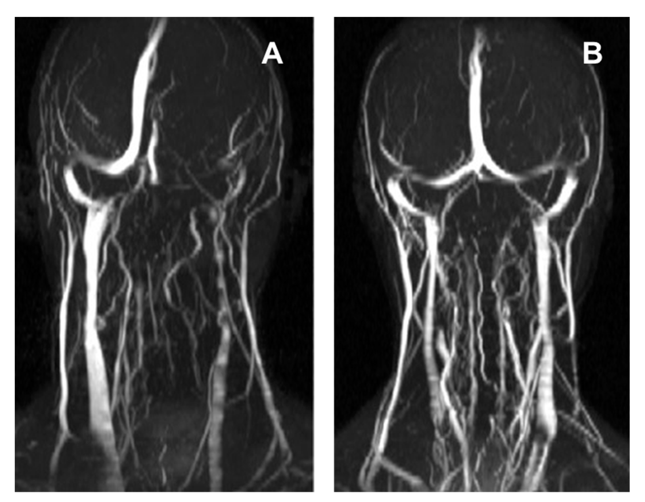
Figure 5.
TOF MR venograph of the neck of: (A) subject 5010, showing turbulent and reduced flow in the left IJV. The aCSF flow for subject 5010 was predicted from the arterial, venous and cCSF flow rates with an r2 = 0.587; and (B) subject 5006, showing extensive collateral rerouting of venous blood. Notwithstanding this, the aCSF for subject 5006 was strongly predicted by the model (r2 = 0.894).


Table 1.
Demographic results for the respective subjects.
| Subject | Age (Yrs) | Sex |
|---|---|---|
| 5002 | 31 | Female |
| 5004 | 28 | Female |
| 5005 | 38 | Male |
| 5006 | 32 | Male |
| 5007 | 37 | Female |
| 5010 | 36 | Male |
| 5011 | 30 | Female |
| 5012 | 60 | Female |
| 5015 | 22 | Female |
| 5016 | 28 | Female |
| 5031 | 21 | Female |
| 5033 | 45 | Male |
| 5035 | 23 | Female |
| Mean | 33.15 | na |
| SD | 10.61 | na |
AVD—arteriovenous delay in milliseconds; cCSF-sv—cervical cerebrospinal fluid stroke volume in microlitres per heart beat; aCSF-sv—aqueductal cerebrospinal fluid stroke volume in microlitres per heart beat; na—not applicable.
Table 2.
Mean, minimum and maximum flow rates (with the computed pulsatility indices) for the cervical arterial, venous and CSF flows, together with aqueductal CSF flow, aggregated for all subjects.
Table 2.
Mean, minimum and maximum flow rates (with the computed pulsatility indices) for the cervical arterial, venous and CSF flows, together with aqueductal CSF flow, aggregated for all subjects.
| Signal | Mean Flow Rate (mL/s) Mean (SD) | Median Flow Rate (mL/s) Mean (SD) | Caudal Peak (mL/s) Mean (SD) | Cranial Peak (mL/s) Mean (SD) | Pulsatility Index Mean (SD) |
|---|---|---|---|---|---|
| Arterial flow rate | 12.34 (2.06) | 11.31 (2.01) | 8.36 (1.55) | 19.58 (4.51) | 0.91 (0.22) |
| Venous flow rate | −12.33 (2.02) | −12.26 (1.98) | −15.71 (2.86) | −8.89 (2.25) | 0.56 (0.23) |
| cCSF flow rate | 0.08 (0.10) | 0.59 (0.45) | −2.70 (1.05) | 1.72 (0.58) | 3.85 (129.86) |
| aCSF flow rate | 0.00 (>0.01) | 0.00 (0.01) | −0.10 (0.06) | 0.09 (0.05) | 31.28 (86.47) |
cCSF—cervical cerebrospinal fluid (CSF) flow rate; aCSF—aqueductal CSF flow rate (i.e., CSF in the aqueduct of Sylvius).
Table 3.
Mean signal correlation r values for all the subjects aggregated together.
| Arterial Flow Rate Mean r Value (SD) | Venous Flow Rate Mean r Value (SD) | cCSF Flow Rate Mean r Value (SD) | aCSF Flow Rate Mean r Value (SD) | |
|---|---|---|---|---|
| Arterial flow rate | - | - | - | - |
| Venous flow rate | -0.601 (0.293) | - | - | - |
| cCSF flow rate | -0.837 (0.126) | 0.621 (0.178) | - | - |
| aCSF flow rate | -0.450 (0.406) | 0.763 (0.266) | 0.539 (0.384) | - |
cCSF—cervical cerebrospinal fluid (CSF) flow rate; aCSF—aqueductal CSF flow rate (i.e., CSF in the aqueduct of Sylvius).
Table 4.
Coefficients and relative importance weights for the respective arterial, venous and cCSF signals, together with the model adjusted r2 values for the respective subjects.
Table 4.
Coefficients and relative importance weights for the respective arterial, venous and cCSF signals, together with the model adjusted r2 values for the respective subjects.
| Arterial | Venous | cCSF | Model | Model | Model | Arterial | Venous | cCSF | ||
|---|---|---|---|---|---|---|---|---|---|---|
| Subject | Intercept | Coef. | Coef. | Coef. | p-value | MSE (mL/s)2 | Adj. r2 | RIW | RIW | RIW |
| 5002 | 0.1941 * | 0.0444 | 0.0596 | 0.0805 | <0.001 | 0.002 | 0.787 | 21.905 | 45.036 | 33.059 |
| 5004 | 0.2413 | −0.0006 * | 0.0204 | −0.0169 * | <0.001 | 0.002 | 0.656 | 31.312 | 57.687 | 11.001 |
| 5005 | 0.1716 | 0.0039 | 0.0179 | 0.0206 | <0.001 | <0.001 | 0.884 | 11.208 | 72.520 | 16.272 |
| 5006 | 0.5092 | −0.0150 | 0.0287 | −0.0178 | <0.001 | <0.001 | 0.894 | 33.611 | 51.167 | 15.221 |
| 5007 | 0.1438 * | 0.0090 * | 0.0247 | 0.0200 * | <0.001 | <0.001 | 0.876 | 6.841 | 84.902 | 8.257 |
| 5010 | −0.0944 * | 0.0150 | 0.0078 * | 0.0455 | <0.001 | 0.006 | 0.587 | 10.934 | 25.313 | 63.753 |
| 5011 | 0.1659 | 0.0050 | 0.0191 | −0.0031 * | <0.001 | <0.001 | 0.856 | 7.072 | 80.327 | 12.601 |
| 5012 | 0.2371 | −0.0129 | 0.0069 | −0.0272 | <0.001 | <0.001 | 0.847 | 39.786 | 44.572 | 15.642 |
| 5015 | 0.0868 | 0.0036 | 0.0094 | 0.0074 | <0.001 | <0.001 | 0.884 | 10.902 | 48.329 | 40.770 |
| 5016 | 0.4050 | −0.0034 * | 0.0340 | 0.0458 * | <0.001 | 0.001 | 0.947 | 21.941 | 43.624 | 34.435 |
| 5031 | 0.0436 * | −0.0004 * | 0.0018 * | −0.0111 | 0.004 | <0.001 | 0.295 | 21.353 | 8.460 | 70.187 |
| 5033 | 0.3757 | 0.0024 * | 0.0399 | 0.0353 | <0.001 | <0.001 | 0.956 | 24.352 | 50.036 | 25.612 |
| 5035 | −0.0446 * | 0.0065 | 0.0037 * | 0.0433 | <0.001 | <0.001 | 0.857 | 28.156 | 23.539 | 48.304 |
| Mean | 0.1873 | 0.0044 | 0.0211 | 0.0171 | <0.001 | 0.002 | 0.794 | 20.721 | 48.886 | 30.393 |
| Median | 0.1716 | 0.0036 | 0.0191 | 0.0200 | <0.001 | 0.001 | 0.857 | 21.905 | 48.329 | 25.612 |
| SD | 0.1728 | 0.0145 | 0.0165 | 0.0320 | <0.001 | 0.001 | 0.184 | 22.027 | 20.415 | 10.705 |
* Not significant at p < 0.05, otherwise all values are significant. AVD—arteriovenous delay; CC—cardiac cycle; MSE—mean square error; RIW—relative importance weighting; cCSF—cervical cerebrospinal fluid (CSF) flow rate.
© 2019 by the authors. Licensee MDPI, Basel, Switzerland. This article is an open access article distributed under the terms and conditions of the Creative Commons Attribution (CC BY) license (http://creativecommons.org/licenses/by/4.0/).
Share and Cite
MDPI and ACS Style
Beggs, C.B.; Shepherd, S.J.; Cecconi, P.; Lagana, M.M. Predicting the Aqueductal Cerebrospinal Fluid Pulse: A Statistical Approach. Appl. Sci. 2019, 9, 2131. https://doi.org/10.3390/app9102131
AMA Style
Beggs CB, Shepherd SJ, Cecconi P, Lagana MM. Predicting the Aqueductal Cerebrospinal Fluid Pulse: A Statistical Approach. Applied Sciences. 2019; 9(10):2131. https://doi.org/10.3390/app9102131
Chicago/Turabian StyleBeggs, Clive B, Simon J Shepherd, Pietro Cecconi, and Maria Marcella Lagana. 2019. "Predicting the Aqueductal Cerebrospinal Fluid Pulse: A Statistical Approach" Applied Sciences 9, no. 10: 2131. https://doi.org/10.3390/app9102131
Note that from the first issue of 2016, this journal uses article numbers instead of page numbers. See further details here.