Development of Operator Theory in the Capacity Adjustment of Job Shop Manufacturing Systems


1
International Graduate School for Dynamics in Logistics, Faculty of Production Engineering, University of Bremen, 28359 Bremen, Germany
2
BIBA Bremer Institut für Produktion und Logistik GmbH, Faculty of Production Engineering, University of Bremen, 28359 Bremen, Germany
*
Authors to whom correspondence should be addressed.
Appl. Sci. 2019, 9(11), 2249; https://doi.org/10.3390/app9112249
Submission received: 30 April 2019
/
Revised: 24 May 2019
/
Accepted: 27 May 2019
/
Published: 31 May 2019
(This article belongs to the Special Issue New Industry 4.0 Advances in Industrial IoT and Visual Computing for Manufacturing Processes)
Abstract
:With the development of industrial manufacture in the context of Industry 4.0, various advanced technologies have been designed, such as reconfigurable machine tools (RMT). However, the potential of the latter still needs to be developed. In this paper, the integration of RMTs was investigated in the capacity adjustment of job shop manufacturing systems, which offer high flexibility to produce a variety of products with small lot sizes. In order to assist manufacturers in dealing with demand fluctuations and ensure the work-in-process (WIP) of each workstation is on a predefined level, an operator-based robust right coprime factorization (RRCF) approach is proposed to improve the capacity adjustment process. Moreover, numerical simulation results of a four-workstation three-product job shop system are presented, where the classical proportional–integral–derivative (PID) control method is considered as a benchmark to evaluate the effectiveness of RRCF in the simulation. The simulation results present the practical stability and robustness of these two control systems for various reconfiguration and transportation delays and disturbances. This indicates that the proposed capacity control approach by integrating RMTs with RRCF is effective in dealing with bottlenecks and volatile customer demands.
1. Introduction
As customer demand is changing quickly, production and logistic systems become more complex and dynamic. Moreover, various delays, stochastic disturbances, and bottlenecks in the production system induce additional challenges for manufacturers. To deal with these problems, numerous advanced technologies, such as reconfigurable machine tools (RMT), Internet of Things (IoT), radio-frequency identification (RFID), and cyber-physical systems (CPS), have been proposed for a more automatic, accurate, and reliable monitoring and controllable manufacturing system [1,2,3]. This displays that the manufacturing industry is on its way toward a new generation, named Industry 4.0 [4]. However, to use these technologies efficiently, effective integration plays a vital role, which has attracted researchers’ increasing attention. Capacity adjustment is one such approach for manufacturing systems, especially for job shop systems, to deal with volatile customer demands. This paper focuses on developing an effective capacity control strategy for the job shop system by means of RMTs.
A job shop system is one production mode with flexible producing paths for a variety of products. Compared with traditional flow shop manufacturing systems with fixed producing paths, job shop systems have the advantage of being able to satisfy changing demand. However, they also have several drawbacks, such as high work-in-process (WIP) levels, high cost, and low productivity [5]. In the literature, some researchers applied scheduling methods to deal with these problems. For example, Wang and Rosenshine [6] discussed the scheduling for combination of made-to-stock and made-to-order jobs in a job shop environment considering mean flowtime. In [7], simulation-based multiobjective optimization as a hyper-heuristic was utilized in the automatic design of scheduling rules for complex job shop systems. Further, other algorithms, such as tabu search [8], genetic algorithm (GA) [9], genetic programming based hyper-heuristic approach (GA-HH) [10], and particle swarm optimization (PSO) [11], were applied to the flexible job shop scheduling problem. The aim of these works was to improve productivity as well as to minimize cost and completion time. Another possibility to solve these problems is capacity adjustment in short- or mid-term horizons [12]. Related work is introduced in the next section.
1.1. Related Research
The methods of capacity adjustment can be classified into two types: Labor-oriented approaches and machinery-oriented approaches. Labor-oriented approaches mainly modify capacity through adjusting the working time. In contrast to these, machinery-oriented approaches adjust capacity through the flexibility of machines. Reconfigurable machine tools (RMT), as one advanced piece of technology of Industry 4.0, provide a new opportunity for machinery-oriented capacity adjustment, which cannot be achieved using classical dedicated machine tools (DMT) only. In [12], RMTs were used in harmonizing the throughput-time capacity control approach to plan the delivery dates and analyze the inventory range of each workstation considering reconfiguration delays. The proportional–integral–differential (PID) control method [13,14] was applied to adjust the capacity, and a mathematical model of job shop systems was developed, including the new application degree of freedom of RMTs. Furthermore, the respective model was continuously extended, including WIP and planned WIP level of each workstation, and a model predictive control (MPC) approach was applied considering time-varying input orders [15]. However, job shop systems are not single-input–single-output (SISO) systems but instead show nonlinear dynamics as well as a multi-input–multi-output (MIMO) structure with strong coupling between the workstations (subsystems). Additionally, these systems also suffer from various disturbances and delays, which are unaccounted for in the literature. Operator-based robust right coprime factorization (RRCF) [16] represents one option to deal with these issues.
Operator theory is an advanced control theoretical approach to effectively control and analyze the dynamic and stability performances of a class of nonlinear systems [17]. Moreover, it is accessible to ensure the stability of nonlinear systems using the Bezout identity [18]. The robust stability and traceability of the nonlinear affine systems with unknown bounded disturbances were analyzed in [19]. The design of robust and tracking controllers of nonlinear feedback systems was considered in [20,21,22,23]. Additionally, this method has been applied to deal with complex problems, such as disturbances, delays, couplings, and so on. In [24], this method was used to deal with internal and external disturbances to ensure robust stability. Deng et al. [25,26] analyzed the delays and faults detection in a thermal process control system using operator theory. In [27], a tracking operator was designed to cope with unknown time-varying delays in nonlinear uncertain systems. Bi and Deng [28,29] solved the coupling problem in MIMO systems and designed robust controllers for MIMO systems. The literature illustrates the effectiveness of the RRCF approach in dealing with nonlinearities, disturbances, delays, and couplings, which occur in job shop systems.
1.2. Research Work
In this paper, the RRCF approach is utilized to design controllers for the capacity adjustment of job shop systems with RMTs and analyze the dynamic and stability performance of the system. In the design of the capacity control system, the WIP level is one key performance indicator, which highly influences cost, throughput, and delivery date reliability [30]. Therefore, our aim was to ensure that the WIP of each workstation is on a planned level. However, the complex material flow, couplings, various delays, and disturbances, including transportation delays between workstations, reconfiguration delays of RMTs, and stochastic demands, make this problem more difficult, especially for large-scale companies. To deal with these challenges, a decoupling controller based on operator theory was applied to transform the complex MIMO system into multiple SISO systems to decrease the complexity for a quick response and less involvement with other workstations [30]. Then, the capacity of each SISO system (workstation) was controlled to ensure the WIP on a planned level. Additionally, to verify the effectiveness of the RRCF control system, PID was considered as the benchmark.
The structure of the paper is organized as follows: In Section 2, the mathematical preliminaries aew introduced. Then, the model of the job shop system with RMTs ia described in Section 3. Thereafter, Section 4 concentrates on the capacity control design, and simulation results are shown in Section 5. Finally, the conclusions and an outlook are provided in Section 6.
2. Mathematical Preliminaries
In this paper, general nonlinear input–output systems of the form:
are considered, where the input and output spaces U and Y are two normed linear spaces over the field of complex numbers, endowed, respectively, with norms and . The set of all (nonlinear) operators is denoted by and call and the domain and range of P. A (semi)-norm on (a subset of) is defined via:
Given such a system, our aim is to show the stability of the system, which is formally defined as follows:
Definition 1
(Finite-Gain Input–Output Stability). An operator with and is called finite-gain input–output stable if:
- 1.
- it is input–output stable, i.e., , and if;
- 2.
- the norm is well defined and finite, i.e., .
Here, and are called the stable input subspace and the stable output subspace of the operator P, respectively. Moreover, an operator P is called causal, stabilizable or unimodular if:
- for the projection: (causal)it has for all and all ;
- there exists an operator such that is input–output stable; (stabilizable)
- P is stabilizable and . (unimodular)
These three properties allow us to introduce our main tool to show finite-gain input–output stability.
Definition 2
(Right Coprime Factorization (RCF)). Let be a causal and stabilizable operator. We say that P has a right coprime factorization illustrated in Figure 1, if there exist finite-gain input–output stable and causal operators , as well as and such that:
- 1.
- D is causal, invertible and holds on , and:
- 2.
- for the unimodular operator , the Bezout identity is:
Here, y, w, and u represent the output, quasi-state, and input signal respectively, cf. [16] for details. v is the reference input, l is the feedback state, and e is the error between v and l. Then, the latter definition allows us to convert the control system (1) to a dynamical system.
Theorem 1.
If a causal and stabilizable operator has right coprime factorization, then the respective closed loop is finite-gain input–output stable. Moreover, for any reference v, the closed loop simplifies to .
Proof.
As P has a right coprime factorization, Figure 1 can be utilized to obtain and . Therefore, we have . Again, by the right coprime factorization property, the Bezout identity (2) can be applied to obtain and .
Hence, by , cf. Figure 2, the second assertion follows.
Regarding finite-gain input–output stability, unimodularity of M and finite-gain input–output stability of N are first utilized to obtain:
which shows input–output stability. Similarly, we obtain by unimodularity of M:
Now, finite-gain input–output stability of N is utilized to conclude , which completes the proof. □
In order to include model uncertainties, the mapping P is modified respectively, i.e., an unknown but bounded operator in parallel is integrated to N.
Definition 3
(Robust Right Coprime Factorization (RRCF)). Consider to be a causal and stabilizable operator with right coprime factorization and suppose a bounded model disturbance to act as shown in Figure 3. Then, P has robust right coprime factorization if the two operators A and B satisfy the Bezout identity , where is a unimodular operator.
Similar to Theorem 1, the closed loop in Figure 3 can be simplified to a dynamical system, cf. Figure 4.
Corollary 1.
If a causal and stabilizable operator has robust right coprime factorization, then the respective closed loop is finite-gain input–output stable. Moreover, for any reference v, the closed loop simplifies to , with from Definition 3.
Proof.
Completely analog to the proof of Theorem 1, where N is replaced by . □
Using these definitions reveals an effective approach to control and analyze the stability and performance of a class of nonlinear control systems, which include job shop systems. Before designing a respective controller, the model of such a system is shortly recapped.
3. Mathematical Model
Job shop manufacturing systems have a high flexibility and can produce numerous types of products, as these may flow flexibly between all workstations. The variables in the model are given in Table 1. In general, for a job shop system with n workstations, the simplified model of the jth () workstation is illustrated in Figure 5. The input rate of the workstation is the sum of output rate from all workstations, including the workstation itself and a possible initial stage. The output rate of the workstation is the current capacity.
The workstation receives orders from the initial stage () and workstations and delivers its products to a final stage () and workstation . Thus, for the jth workstation, considering the transportation delay between each workstations, the orders input rate is:
where is the order input from the initial stage. The order output rate of the jth workstation is given by:
where the flow probabilities satisfy for all . The current WIP as the output signal of the jth workstation is the integral difference between the order input and output rate plus disturbances over time:
The latter variable is of particular importance as for a high level of WIP. The order output rate is equal to the capacity of the workstation, that is:
In order to reflect the functionality of RMTs for capacity adjustment, in [31], an extended model of a job shop system with DMTs and RMTs was proposed, cf. Figure 5 for a sketch of workstation j with an assigned number of RMTs. Due to the high productivity of DMTs, this kind of machines will also be adopted in the system. The overall system includes reconfigurable and dedicated machine tools. Here, all RMTs can be used within all workstations but only perform one operation in the specific period. Moreover, each DMT can only perform one operation and is assigned to a specific workstation. Hence, each workstation consists of a fixed number of DMTs and a variable number of RMTs. Therefore, the maximal capacity of a workstation is given by:
The number of RMTs in each workstation is considered to be our new degree of freedom. If the association of an RMT to a workstation is changed over time via , this renders the maximal capacity time-variant. Assuming a high WIP, each workstation is operating at its maximal capacity, and its output rate is given by:
where is the reconfiguration delay when RMTs change the operation between workstations. Note that if an RMT is reconfigured from workstation j to workstation k, the capacity of workstation k increases only after a lag (e.g., 2 h), while the capacity of workstation j decreases immediately. This reveals the description:
Then, the WIP level can be controlled via the function for all workstations in (5). The input–output model of the system, which is the plant operator for , is given by:
where and , for all .
Additionally, the number of RMTs in the system is assumed to be limited by , and each workstation contains at least 0 RMTs. This reveals the control constraints:
Note that similar to but in contrast to the input and output rate values and , our control is integer instead of continuous. To compensate for the issue, the truncation is utilized. Moreover, for the constraint , the fractional approach [32] is utilized, which is given as:
Note that if the number of utilized RMTs does not exceed the total number of RMTs, then corresponds to the truncated value of . Otherwise, the fractional discrete value of RMTs in the sum over all workstations is considered.
Note that model (9) only applies if the system is working at a high WIP level. In this case, the order output rate equals the maximum capacity, i.e., the WIP level can be controlled via the assignment of RMTs for all workstations.
4. Capacity Control
Based on the mathematical preliminaries and model from the previous sections, RRCF was used to control the capacity of the job shop systems. According to [26], the right factorization of the job shop system for is obtained as:
In this description, couplings, delays, and disturbances render the system more complex. In practice, operators have to consider all workstations to assign RMTs, which impacts on efficiency. In order to decrease complexity, a decoupling design allows responding quickly with less involvement from other workstations. Firstly, a decoupling controller was designed to split the MIMO system into multiple SISO systems. Then, the RRCF and tracking controllers for each SISO system were derived to ensure the WIP of workstations remains on the predefined levels.
4.1. Decoupling Control
In (11), there exist couplings between all workstations, which can be described as n linear equations. Solving the n linear systems:
is obtained. To avoid the difficult computation of an RRCF control for the MIMO system, decoupling as proposed in [29] was utilized to transfer it into multiple SISO systems. To obtain n independent SISO systems, the decoupling operators H and G as shown in Figure 6 need to satisfy the following theorem, cf. Theorem 1 in [29].
Theorem 2
(Decoupled RRCF Control). If is linear and:
then the MIMO system is decoupled and is stable and invertible. Here, ) represents the decoupling operator with .
Applying the latter to the job shop system, the following proposition can be concluded.
Proposition 1
(Decoupled RRCF Control for Job Shop System). Consider a plant (9) as well as decoupling parameters with for and let be the identity operator, unimodular for , such that:
holds. Then:
holds. Additionally, if is sufficient large, then is stable and invertible.
Proof.
As are the identity operators and unimodular operators for , then plant (9) has:
As , it is a linear operator. Additionally, considering is sufficient large, is invertible. Its norm is:
As and the production rate of RMTs is a positive constant, hence, . Thus, from Definition 1, this operator is stable, showing the assertion. □
4.2. RRCF Control
After the decoupling, the RRCF control for each SISO system was considered separately. Based on Definition 3, the RRCF operators and (cf. Figure 7) can be designed following the Bezout identity:
Here, for simplicity of exposition, the form:
is chosen to satisfy the sufficient condition with , where is the RRCF control parameter for . Then, let , and from (12) and (15), we obtain:
Then, Corollary 1 can be applied to show the finite-gain input–output stability of the system.
4.3. Tracking Control
The RRCF control system has been designed to ensure finite-gain input–output stability but does not consider the tracking performance of the job shop system. In order to ensure the WIP can track a given level, a tracking controller as proposed in [24] was integrated, cf. Figure 8 for a sketch. Here, for simplicity of exposition, the tracking controller was designed as:
where and are tracking parameters. By setting the parameters appropriately, the tracking controller can minimize the error between the desired and actual WIP level.
In all, the capacity control of a job shop system includes three parts: Firstly, the decoupling controllers and work on dealing with couplings between each workstation and transferring the complex MIMO system into multiple SISO systems. The second part is RRCF control of each SISO system (workstation), where RRCF controllers and are designed to ensure finite-gain input–output stability. Based on the stability, tracking controllers are considered to guarantee that the WIP levels of all workstations track predefined levels. Including these adaptations of the decoupling, RRCF, and tracking controllers, this method can be utilized as a capacity adjustment method using RMTs in our job shop setting.
5. Case Study
To evaluate our proposed RRCF controller, a four-workstation three-product job shop system with RMTs was considered. This case was defined in [33,34] in mould making. The flow probabilities for the three different products , , given by present the order output rate of product i from workstation j to workstation k (for ) and the final stage for , cf. Figure 9. It changes dynamically with the varying input rates. The parameter settings are shown in Table 2. Additionally, the PID control approach, cf. [32], was chosen as a benchmark for the RRCF control system. Here, two scenarios were considered in the simulation implemented in MATLAB. The performance of RRCF and PID control systems for constant and stochastic demands was analyzed sequentially.
5.1. Simulations for Constant Demands
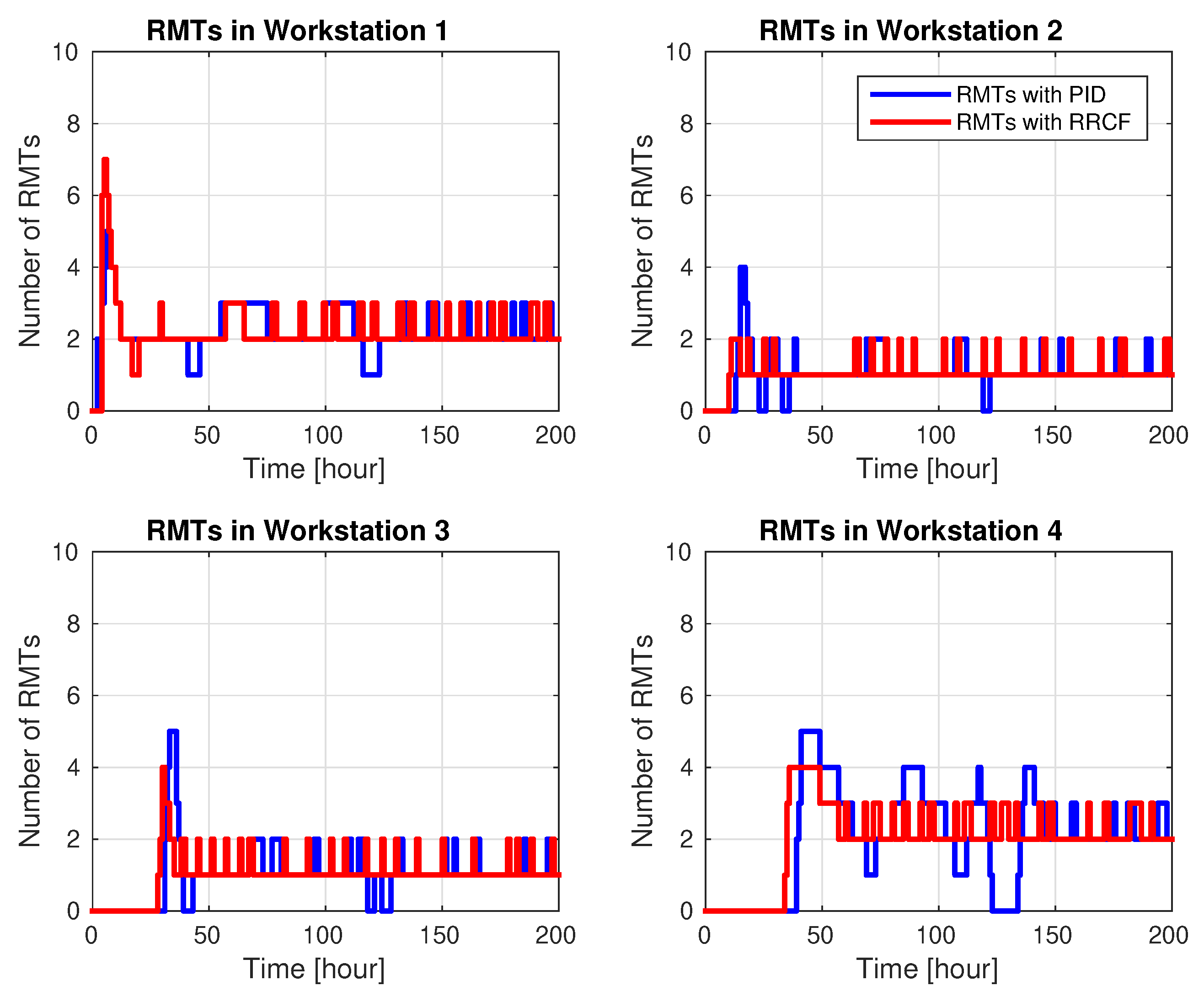
Considering constant customer demands, the resulting performances of all workstations with delays are shown in Figure 10, Figure 11 and Figure 12. The allocation of respective RMTs at each workstation is illustrated in Figure 10. The error between the planned and current WIP level of each workstation is given in Figure 11. The red and blue lines represent the variables with PID and RRCF control, respectively. The performance of WIP levels and distribution of RMTs of each workstation in this dynamical capacity control process is analyzed as follows.
At workstation 1, due to rush orders from the initial stage, the WIP level in workstation 1 increased and induced bottlenecks in the first 5 h, so the error in Figure 11 was highly decreased. Then both PID and RRCF controllers started assigning RMTs to this workstation, cf. Figure 10. Because of the reconfiguration delay, RMTs did not work for the first two hours, so the WIP was still increasing. However, after 2 h, PID and RRCF assigned 5 and 7 RMTs to this workstation, respectively, so the WIP in the RRCF case decreased more than in the PID one. After 10 h, the WIP of workstation 1 was lower than the planned level, so the number of RMTs was decreased. After around 50 h, the WIP in the RRCF case was practically stabilized (cf. [35], Chapter 2 for details), and the respective number of RMTs was also controlled between 2 to 3. The number of RMTs as the input signal is an integer, so the value of the WIP showed scattering but bounded behavior. For the PID case, the WIP level was practically stabilized after 130 h with higher overshoot.
At workstation 2, the initial WIP was lower than the planned level, so the error between planned and current WIP at the beginning was positive. In the first two hours, the error increased a bit due to fewer input orders from Workstation 1. After 2 h, owing to more orders flowing in from Workstation 1 but limited capacity, the WIP level was quickly increased and the error decreased quickly in the first 10 h in Figure 11. Therefore, bottleneck also moved to this workstation. After 10 h, both controllers started assigning RMTs to workstation 2 to solve the bottleneck in Figure 10. However, the RRCF had a quicker response with fewer than 2 RMTs to practically stabilize the WIP levels after 30 h, while the PID showed a slower response and took 4 RMTs to resolve the bottleneck. Additionally, the respective WIP level displayed higher overshoot and longer settling time than the RRCF control.
At workstations 3 and 4, the initial WIPs were less than the planned levels, so the initial error was positive in Figure 11. In the first two hours, as there was less order input and more output rate, the WIP level decreased, so the errors increased a bit. Then, due to increasing order inputs but limited capacity, the WIPs increased quickly over the planned levels and induced bottlenecks. After around 30 and 40 h at Workstations 3 and 4, respectively, both PID and RRCF controllers assigned RMTs to these two workstations. Then, the capacities increased, while the WIP levels decreased. However, the WIPs in RRCF were quickly stabilized and close to the planned levels. Same as for workstation 2, the RRCF control system showed a quicker response and used fewer RMTs than the PID control system to solve the bottlenecks. Moreover, the WIP levels of these two workstations within the RRCF control tended to be practically stable after 50 h, while the PID control system took around 150 h for the practical stabilization of the WIP levels. Additionally, the PID control showed higher overshoots and more oscillations. In Figure 10 and Figure 11, both the PID and RRCF control approaches could practically stabilize the WIP level of all workstations. Nonetheless, RRCF showed better transient and steady state performance than the PID control system.
After the performance analysis of each workstation, the performance of each product was further analyzed. Figure 12 illustrates the order input and output rate of each product. The order input rate of each product was 51 per hour in red line. In Figure 9, all products were finished at workstation 3 or 4. Due to a capacity shortage, cf. Figure 10, the output rates of all products were mostly lower than the input rates for the first 30 h. Later, the order output rate of each product also showed scattering but bounded behavior for both PID and RRCF control. However, the RRCF control in green lines showed fewer overshoots and shorter settling time than the PID control in blue lines. This indicates that both the PID and the proposed RRCF method can practically stabilize the constant demand. However, compared to the PID control, the RRCF control has a quicker response to practically stabilize the system with fewer overshoots.
5.2. Simulations for Stochastic Demands
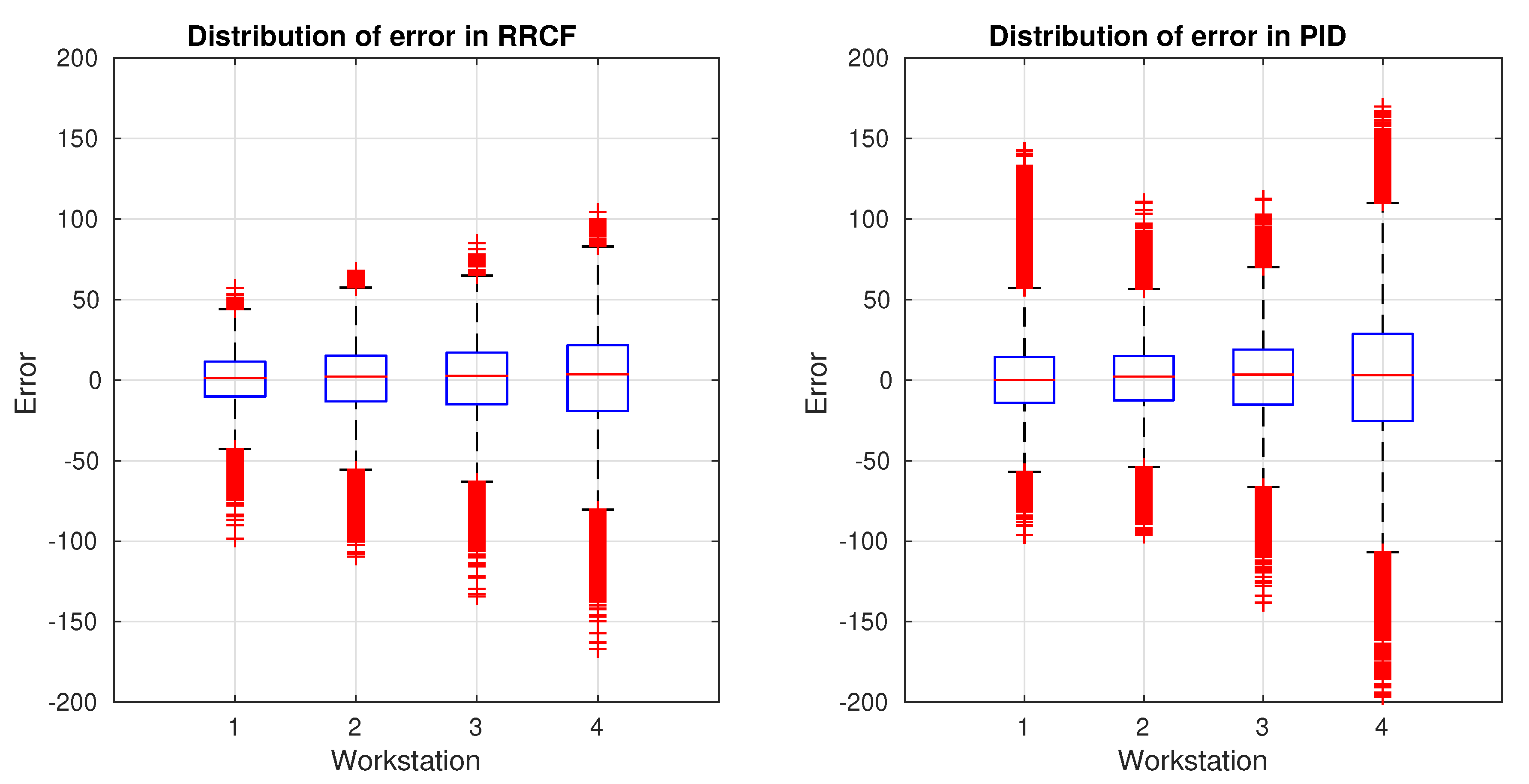
Here, the demands of each product were assumed to be normally distributed with a mean value of 51 and variance of 5. Then, the practical stabilized closed loop was simulated 1000 times, and then the distribution of errors between the planned and current WIP at each workstation was obtained. The respective results are shown in Figure 13. This demonstrated that the mean errors of each workstation within the PID and RRCF control were almost close to zero. However, the distribution of the error in the RRCF control system is smaller than that for PID. Additionally, as to the number of RMTs and the absolute errors of each workstation, the mean values , and the standard deviation , are given in Table 3. At this time, the mean and standard deviation of the absolute errors in the RRCF control are less than the PID control most time. This illustrated that the RRCF control system is more robust than the PID one. Concerning the assignment of RMTs, there is no difference between both control systems on the mean value of RMTs, while RRCF showed higher values on standard deviation. This indicated that the proposed RRCF capacity control method can deal with the stochastic demands and showed higher robustness than the PID control method.
6. Conclusions and Outlook
In this paper, an operator-based approach incorporating RMTs was developed to control the capacity of job shop systems. A mathematical model integrating the flexibility of RMTs was presented for the capacity control. The design of the RRCF controller was discussed in the capacity control of a general job shop system. To evaluate the effectiveness of the RRCF control approach, a PID control was applied as a benchmark in the simulation of a four-workstation job shop manufacturing system. Then, conclusions are summarized as follows:
- The proposed RRCF capacity control method can deal with the constant demands and solve bottlenecks to ensure practical stability of the system in the WIP levels of all workstations and the output rates of all products. Additionally, compared to the PID method, the RRCF showed better transient and steady state performances, with shorter settling times and lower overshoots.
- For the stochastic demands, Monte Carlo simulation was utilized to evaluate the robustness of these two control systems. The simulation results illustrated that RRCF was more robust than PID with less mean and standard deviation of the absolute errors between planned and current WIP levels.
- The simulation results also supported the applicability and effectiveness of the proposed capacity control approach by integrating of RMTs with the RRCF method.
- As this capacity control approach is in a decentralized architecture, it also can be used in large-scale job shop systems.
In future work, the following research directions can be considered:
- The mathematical model can be further extended and integrated with more performance indicators, e.g., backlog and inventory for more complex problems with various perspectives.
- The proposed capacity control approach is designed from the customer perspective. Another work can be to develop an effective reconfiguration rule to optimize the performance, at the same time satisfying the demands.
Author Contributions
Validation, P.L., Q.Z. and J.P.; Writing—Original Draft Preparation, P.L. and Q.Z.; Writing—Review & Editing, P.L., Q.Z. and J.P.; Supervision, J.P.
Funding
This research was funded by the FUSION and gLINK programs of ERASMUS MUNDUS grant number 2013-2541/001-011-EM and 2014-0861/001-001-EM, respectively.
Acknowledgments
The publication of this paper was supported by Staats- und Universitaetsbibliothek Bremen (SuUB), Germany.
Conflicts of Interest
The authors declare no conflict of interest.
References
- Landers, R.G.; Min, B.K.; Koren, Y. Reconfigurable machine tools. CIRP Ann. Manuf. Technol. 2001, 50, 269–274. [Google Scholar] [CrossRef]
- Huang, G.Q.; Zhang, Y.; Jiang, P. RFID-based wireless manufacturing for real-time management of job shop WIP inventories. Int. J. Adv. Manuf. Technol. 2008, 36, 752–764. [Google Scholar] [CrossRef]
- Atzori, L.; Iera, A.; Morabito, G. The Internet of Things: A survey. Comput. Netw. 2010, 54, 2787–2805. [Google Scholar] [CrossRef]
- Almada-Lobo, F. The industry 4.0 revolution and the future of manufacturing execution systems (MES). J. Innov. Manag. 2015, 3, 16–21. [Google Scholar] [CrossRef]
- Georgiadis, P.; Michaloudis, C. Real-time production planning and control system for job-shop manufacturing: A system dynamics analysis. Eur. J. Oper. Res. 2012, 216, 94–104. [Google Scholar] [CrossRef]
- Wang, M.F.; Rosenshine, M. Scheduling for a combination of made-to-stock and made-to-order jobs in a job shop. Int. J. Prod. Res. 1983, 21, 607–616. [Google Scholar] [CrossRef]
- Freitag, M.; Hildebrandt, T. Automatic design of scheduling rules for complex manufacturing systems by multi-objective simulation-based optimization. CIRP Ann. Manuf. Technol. 2016, 65, 433–436. [Google Scholar] [CrossRef]
- Shen, L.; Dauzère-Pérès, S.; Neufeld, J.S. Solving the flexible job shop scheduling problem with sequence-dependent setup times. Eur. J. Oper. Res. 2018, 265, 503–516. [Google Scholar] [CrossRef]
- Lu, P.H.; Wu, M.C.; Tan, H.; Peng, Y.H.; Chen, C.F. A genetic algorithm embedded with a concise chromosome representation for distributed and flexible job-shop scheduling problems. J. Intell. Manuf. 2015, 29, 1–16. [Google Scholar] [CrossRef]
- Park, J.; Mei, Y.; Nguyen, S.; Chen, G.; Zhang, M. An investigation of ensemble combination schemes for genetic programming based hyper-heuristic approaches to dynamic job shop scheduling. Appl. Soft Comput. J. 2018, 63, 72–86. [Google Scholar] [CrossRef]
- Nouiri, M.; Bekrar, A.; Jemai, A.; Niar, S.; Ammari, A.C. An effective and distributed particle swarm optimization algorithm for flexible job-shop scheduling problem. J. Intell. Manuf. 2018, 29, 603–615. [Google Scholar] [CrossRef]
- Scholz-Reiter, B.; Lappe, D.; Grundstein, S. Capacity adjustment based on reconfigurable machine tools—Harmonising throughput time in job-shop manufacturing. CIRP Ann. Manuf. Technol. 2015, 64, 403–406. [Google Scholar] [CrossRef]
- Kim, J.H.; Duffie, N.A. Design and analysis of closed-loop capacity control for a multi-workstation production system. CIRP Ann. Manuf. Technol. 2005, 54, 455–458. [Google Scholar] [CrossRef]
- Liu, P.; Zhang, Q.; Pannek, J. Capacity adjustment of job shop manufacturing systems with RMTs. In Proceedings of the 10th International Conference on Software, Knowledge, Information Management & Applications (SKIMA), Chengdu, China, 15–17 December 2016. [Google Scholar] [CrossRef]
- Zhang, Q.; Liu, P.; Pannek, J. Modeling and predictive capacity adjustment for job shop systems with RMTs. In Proceedings of the 25th Mediterranean Conference on Control and Automation, Valletta, Malta, 3–6 July 2017. [Google Scholar] [CrossRef]
- Chen, G.; Han, Z. Robust right coprime factorization and robust stabilization of nonlinear feedback control systems. IEEE Trans. Automat. Control 1998, 43, 1505–1509. [Google Scholar] [CrossRef]
- de Figueiredo, R.J.P.; Chen, G. Nonlinear Feedback Control Systems: An Operator Theory Approach; Academic Press Professional, Inc.: San Diego, CA, USA, 1993. [Google Scholar]
- Deng, M. Operator-based Nonlinear Control Systems: Design and Applications; John Wiley & Sons: Hoboken, NJ, USA, 2014. [Google Scholar]
- Wen, S.; Deng, M.; Ohno, Y.; Wang, D. Operator-based robust right coprime factorization design for planar gantry crane. In Proceedings of the IEEE International Conference on Mechatronics and Automation, Xi’an, China, 4–7 August 2010; pp. 1–5. [Google Scholar] [CrossRef]
- Bi, S.; Deng, M. Operator-based robust control design for nonlinear plants with perturbation. Int. J. Control 2011, 84, 815–821. [Google Scholar] [CrossRef]
- Bu, N.; Deng, M. System design for nonlinear plants using operator-based robust right coprime factorization and isomorphism. IEEE Trans. Automat. Control 2011, 56, 952–957. [Google Scholar] [CrossRef]
- Wen, S.; Deng, M.; Inoue, A. Operator-based robust non-linear control for gantry crane system with soft measurement of swing angle. Int. J. Model. Identif. Control 2012, 16, 86–96. [Google Scholar] [CrossRef]
- Wen, S.; Liu, P.; Wang, D. Optimal tracking control for a peltier refrigeration system based on PSO. In Proceedings of the International Conference on Advanced Mechatronic Systems, Kumamoto, Japan, 10–12 August 2014; pp. 567–571. [Google Scholar] [CrossRef]
- Deng, M.; Inoue, A.; Ishikawa, K. Operator-based nonlinear feedback control design using robust right coprime factorization. IEEE Trans. Automat. Control 2006, 51, 645–648. [Google Scholar] [CrossRef]
- Deng, M.; Inoue, A.; Edahiro, K. Fault detection in a thermal process control system with input constraints using a robust right coprime factorization approach. Proc. Inst. Mech. Eng. Part J. Syst. Control Eng. 2007, 221, 819–831. [Google Scholar] [CrossRef]
- Deng, M.; Inoue, A. Networked non-linear control for an aluminum plate thermal process with time-delays. Int. J. Syst. Sci. 2008, 39, 1075–1080. [Google Scholar] [CrossRef]
- Bi, S.; Deng, M.; Wen, S. Operator-based output tracking control for non-linear uncertain systems with unknown time-varying delays. IET Control Theory Appl. 2011, 5, 693–699. [Google Scholar] [CrossRef]
- Deng, M.; Bi, S. Operator-based robust nonlinear control system design for MIMO nonlinear plants with unknown coupling effects. Int. J. Control 2010, 83, 1939–1946. [Google Scholar] [CrossRef]
- Bi, S.; Xiao, Y.; Fan, X. Operator-based robust decoupling control for MIMO nonlinear systems. In Proceedings of the 11th World Congress on Intelligent Control and Automation, Shenyang, China, 29 June–4 July 2014; pp. 2602–2606. [Google Scholar] [CrossRef]
- Lödding, H.; Yu, K.W.; Wiendahl, H.P. Decentralized WIP-oriented manufacturing control (DEWIP). Prod. Plan. Control 2003, 14, 42–54. [Google Scholar] [CrossRef]
- Liu, P.; Pannek, J. Operator-based capacity control of job shop manufacturing systems with RMTs. In Dynamics in Logistics; Springer: Cham, Switzerland, 2018; pp. 264–272. [Google Scholar] [CrossRef]
- Liu, P.; Chinges, U.; Zhang, Q.; Pannek, J. Capacity control in disturbed and time-delayed job shop manufacturing systems with RMTs. IFAC-PapersOnLine 2018, 51, 807–812. [Google Scholar] [CrossRef]
- López de Lacalle, L.N.; Lamikiz, A.; Salgado, M.A.; Herranz, S.; Rivero, A. Process planning for reliable high-speed machining of moulds. Int. J. Prod. Res. 2002, 40, 2789–2809. [Google Scholar] [CrossRef]
- López De Lacalle, L.N.; Lamikiz, A.; Muñoa, J.; Sánchez, J.A. The CAM as the centre of gravity of the five-axis high speed milling of complex parts. Int. J. Prod. Res. 2005, 43, 1983–1999. [Google Scholar] [CrossRef]
- Grüne, L.; Pannek, J. Nonlinear Model Predictive Control: Theory and Algorithms; Springer International Publishing: Cham, Switzerland, 2017. [Google Scholar] [CrossRef]
Figure 1.
Nonlinear feedback control system.

Figure 2.
Input–output system equivalent to Figure 1.
Figure 2.
Input–output system equivalent to Figure 1.
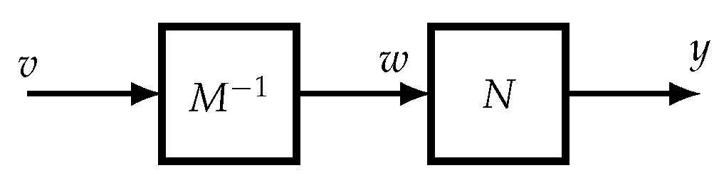
Figure 3.
Nonlinear feedback system with disturbances.
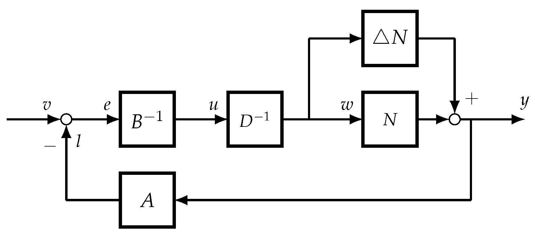
Figure 4.
Equivalent of Figure 3.
Figure 4.
Equivalent of Figure 3.
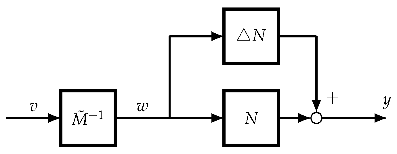
Figure 5.
Model of jth workstation with reconfigurable machine tools (RMTs).

Figure 6.
Decoupling control of multi-input–multi-output (MIMO) system.
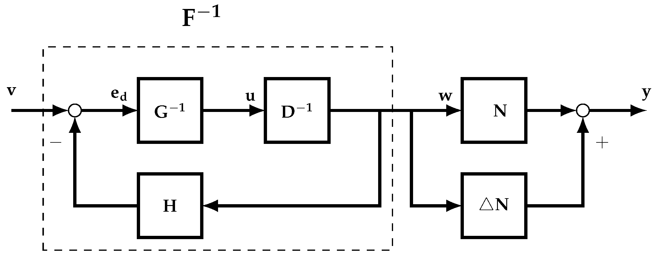
Figure 7.
Robust right coprime factorization (RRCF) control of decoupled MIMO systems.

Figure 8.
Nonlinear feedback tracking control of MIMO system.
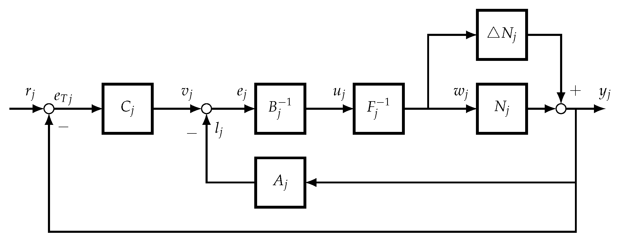
Figure 9.
Four-workstation job shop manufacturing system with RMTs.
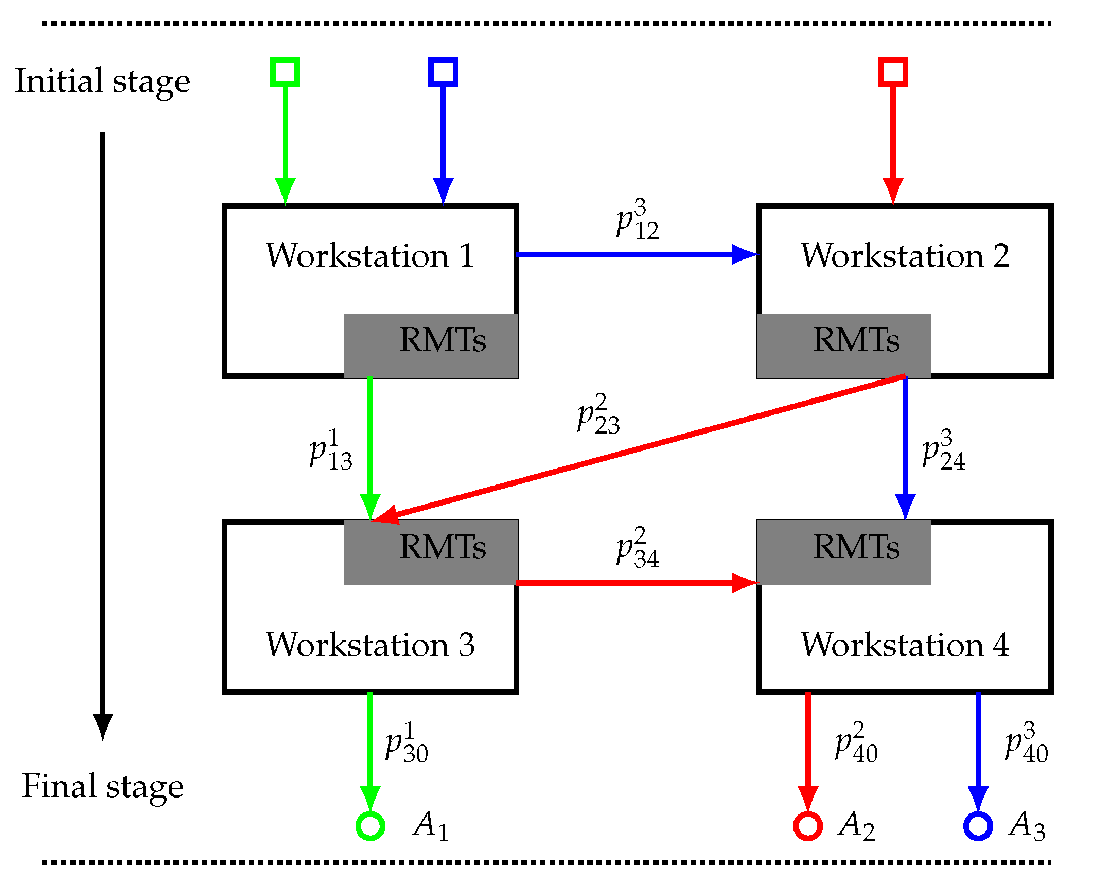
Figure 10.
Number of RMTs in each workstation for constant demands.

Figure 11.
Error between planed and current WIP of each workstation for constant demands.
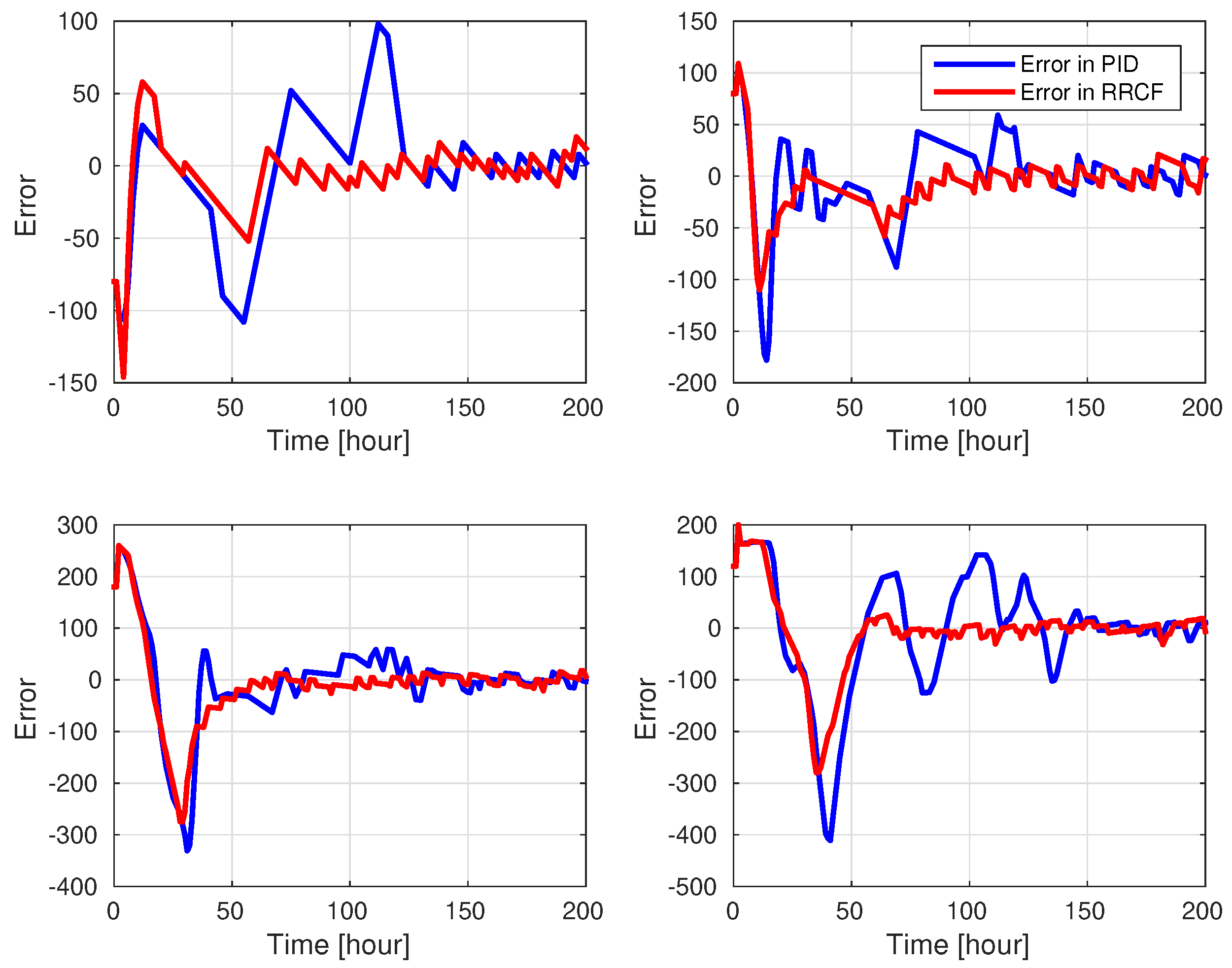
Figure 12.
Order input and output rate of each product for constant demands.
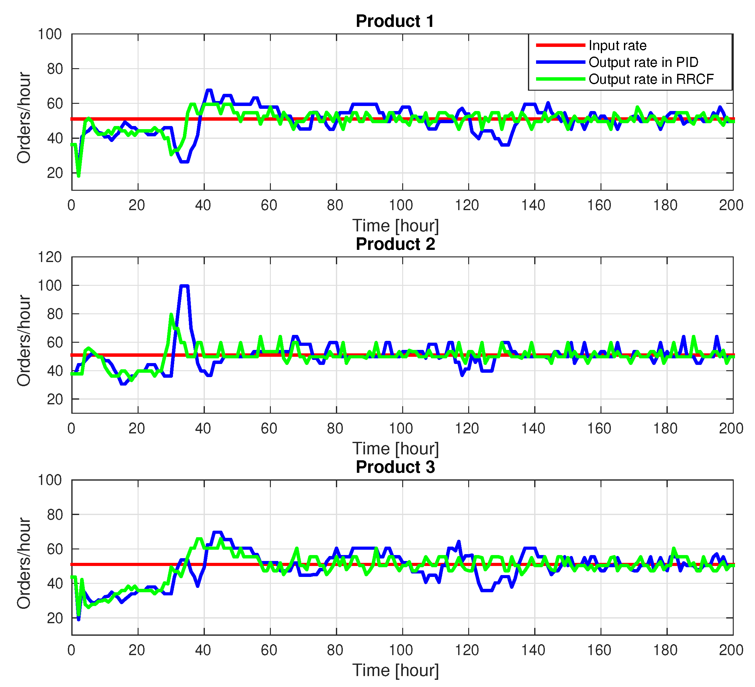
Figure 13.
Distribution of errors at each workstation for stochastic demands.

Table 1.
Variables within the workstation with RMTs.
| Variable | Description |
|---|---|
| Orders input rate from workstation k to workstation j for | |
| Orders input rate of workstation | |
| Orders output rate of workstation j to workstation k for | |
| Orders output rate of workstation | |
| Input signal of workstation , which is equal to the number of RMTs | |
| Output signal of workstation , which is the WIP level of the workstation | |
| Current capacity of workstation | |
| Maximum capacity of workstation | |
| Flow probability that the output orders from workstation j to workstation k for | |
| Number of RMTs in the system | |
| Number of RMTs in workstation | |
| Number of DMTs in workstation | |
| Production rate of DMTs in workstation | |
| Production rate of RMTs in workstation | |
| Disturbances in workstation | |
| Reconfiguration delay | |
| Transportation delay | |
| n | Number of workstations in the system |
Table 2.
Parameter settings of the four-workstation system.
| Number of Workstation | 1 | 2 | 3 | 4 |
|---|---|---|---|---|
| Initial WIP level | 400 | 400 | 300 | 200 |
| Planned WIP level | 240 | 400 | 400 | 240 |
| Number of DMTs | 4 | 2 | 2 | 4 |
| Production rate of DMTs | 20 | 40 | 40 | 20 |
| Production rate of RMTs | 10 | 20 | 20 | 10 |
Table 3.
Performances of system for stochastic demands.
| Controller | PID | RRCF | ||||||
|---|---|---|---|---|---|---|---|---|
| Workstation | 1 | 2 | 3 | 4 | 1 | 2 | 3 | 4 |
| 2.20 | 1.10 | 1.10 | 2.19 | 2.20 | 1.10 | 1.11 | 2.19 | |
| 0.56 | 0.54 | 0.63 | 0.97 | 1.12 | 0.76 | 0.86 | 1.96 | |
| 17.58 | 17.00 | 21.26 | 32.76 | 13.11 | 17.33 | 19.48 | 24.58 | |
| 14.41 | 13.46 | 17.00 | 25.56 | 10.28 | 13.71 | 15.25 | 19.03 | |
© 2019 by the authors. Licensee MDPI, Basel, Switzerland. This article is an open access article distributed under the terms and conditions of the Creative Commons Attribution (CC BY) license (http://creativecommons.org/licenses/by/4.0/).
Share and Cite
MDPI and ACS Style
Liu, P.; Zhang, Q.; Pannek, J. Development of Operator Theory in the Capacity Adjustment of Job Shop Manufacturing Systems. Appl. Sci. 2019, 9, 2249. https://doi.org/10.3390/app9112249
AMA Style
Liu P, Zhang Q, Pannek J. Development of Operator Theory in the Capacity Adjustment of Job Shop Manufacturing Systems. Applied Sciences. 2019; 9(11):2249. https://doi.org/10.3390/app9112249
Chicago/Turabian StyleLiu, Ping, Qiang Zhang, and Jürgen Pannek. 2019. "Development of Operator Theory in the Capacity Adjustment of Job Shop Manufacturing Systems" Applied Sciences 9, no. 11: 2249. https://doi.org/10.3390/app9112249
Note that from the first issue of 2016, this journal uses article numbers instead of page numbers. See further details here.