Article

Algorithm for Surfaces Profiles and Thickness Variation Measurement of a Transparent Plate Using a Fizeau Interferometer with Wavelength Tuning

1
Lab of Applied Optics and Metrology, Department of Precision Mechanical Engineering, Shanghai University, Shanghai 200072, China
2
School of Mechanical and Aerospace Engineering, Nanyang Technological University, Singapore 639798, Singapore
3
Department of Physics, Chemistry and Biology, Linköping University, SE-581 83 Linköping, Sweden
*
Author to whom correspondence should be addressed.
Appl. Sci. 2019, 9(11), 2349; https://doi.org/10.3390/app9112349
Submission received: 8 April 2019 / Revised: 31 May 2019 / Accepted: 4 June 2019 / Published: 7 June 2019
(This article belongs to the Special Issue Precision Dimensional Measurements)

Abstract

:

Featured Application

The proposed method is used to separate the overlapped interferograms formed by parallel interfaces, specifically, surfaces of a transparent plate, and to obtain the front and rear surface profiles, as well as the thickness, simultaneously.

Abstract

An interferogram obtained from a transparent plate contains information on the profiles of both surfaces and on the thickness variation. The present work is devoted to the processing of interferograms of this type. The processing technique is based on a 36-step algorithm developed by the authors for characterization of transparent plates having approximately equal reflections from both sides. The algorithm utilizes weighted multi-step phase shifting that enables one not only separately to extract the front and rear surface profiles together with the thickness variation of the tested plate but also to suppress the coupling errors between the higher harmonics and phase-shift deviation. The proposed measuring method was studied on a wavelength tunable Fizeau interferometer. The tested sample had an optical thickness and surface profile deviations equal to 0.51 µm, 1.38 µm and 0.89 µm, respectively. According to the results obtained using 10 repeated measurements, the root mean square (RMS) errors for determining both surface profiles did not exceed 1.5 nm. Experimental results show that the setup and presented 36-step algorithm are suitable for the measurement of a transparent plate of arbitrary thickness.

1. Introduction

Being an optical element, transparent plates play an essential role in a large variety of optical components and applications [1,2]. The front and rear surface profiles together with the optical thickness are among the fundamental characteristics of a transparent plate. Precise control and monitoring of these characteristics by non-destructive and non-contact methods for samples with different sizes and thickness are often important from a technological point of view and are associated with the quality improvement of finished products. Several optical techniques have been developed for the determination of the thickness. Most of them are based on principles of ellipsometry and interferometry [3,4]. For example, these include the excess fraction method, digital phase-measuring interferometry [5], Fourier transform profilometry [6], random tilt phase-shifting [7], and 3D profilometry based on modulation measurement [8]. White-light interferometry and confocal microscopy have also been used for optical thickness and profile measurement of transparent plates [9,10,11,12].
Depending on the spectrum of the light source used, the methods applied to measure thickness variation can be classified as monochromatic or spectral. The experimental setups of some of those methods include both a monochromatic laser and a spectral halogen lamp [13]. One of the disadvantages of using confocal microscopy is the limitation in the diameter of an observing aperture.
In addition, it is not suitable for measuring the distributions of the surface profiles and the thickness because this method is based on an assumption that a sample has a uniform thickness, it measures the sample on a point by point basis. White-light interferometry is time-consuming and involves a limited aperture. Moreover, the determination of large thicknesses requires a light source possessing a large coherence length.
Wavelength tuning interferometry (WTI) [14,15,16,17,18,19,20,21,22,23,24,25] is an effective method for application in surface metrology, which is primarily limited to front-surface reflected optical element measurements. WTI has also been exploited for separating overlapped interference signals formed by the reference surface of the interferometer used and both surfaces of the measured transparent plate in frequency domain. However, the WTI method [
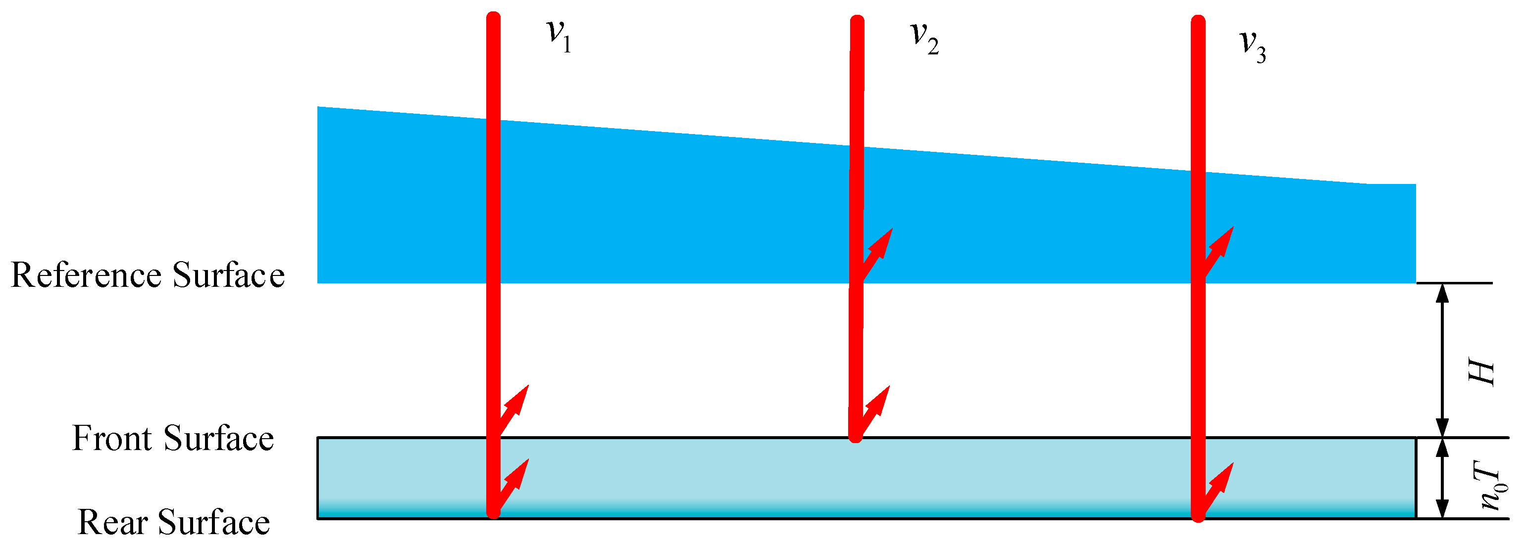
16] provides an air-gap length (the distance between the reference surface at Fizeau geometry to the front surface, Figure 1) which is less than the thickness of the sample. In order to facilitate its application in actual industrial measurements, the air-gap length must be large. In this case, it becomes difficult to measure a sample with a thickness less than 10 mm in an actual measurement process that uses Fizeau interferometer. Whereas a conventional phase-shifting interferometer [26] requires a stable phase detection method for only a single signal obtained from the surface to be tested. The challenge for a wavelength tuning interferometer is an extraction of information in several signal frequencies, when it is necessary to suppress the noise from the neighboring frequency signals.
In this study, we report a developed interferometric phase-shifting method based on a 36-step algorithm to compensate for the phase-shift miscalibration and to suppress the signal contributions from other surfaces. Our algorithm for data processing realizes the separation of multi-surface superposition information. The method utilizes the spectral stretching of the Discrete Fourier Transform function and is meant to be used for measurements of transparent plates with arbitrary thicknesses. The experimental setup is based on the Fizeau interferometer with wavelength tuning.

2. Materials and Methods

When a beam of light is incident on a transparent plate, an interference pattern is obtained due to multiple reflections from the plate’s surfaces. In order to measure the profile of the transparent plate, it is necessary to extract from the registered interference pattern information caused by each surface [5]. The intensity distribution in the interferogram formed by transparent plate can be expressed as:
I ( x , y , k ) = A 0 + n = 1 A n cos ( φ n ( x , y ) + 2 π v n k ) ,
where I ( x , y , k ) is the intensity of the kth record image in the coordinate ( x , y ) , where the coordinate plane x , y is parallel to the measured interfaces. A 0 is the intensity of the background, and A n is a contrast associated with intensity of the nth harmonic. φ n is the phase of the nth harmonic components, which corresponds to the path difference between the sample surface and the reference surface of the interferometer. The accuracy (peak-to-valley value) is less than one twentieth of the wavelength, λ / 20 , generally. The modulation frequency is v n and is proportional to the optical path difference (OPD) of each pair of interfering fringe.
For the signal generated by the interference due to the reflection from the reference and front-and-rear surfaces, the frequency v is given by:
v = 2 O P D λ 0 2 · d λ d k ,
where λ 0 is the central wavelength of the laser source, and d λ d k is the wavelength-tuning rate per time unit.
In Figure 1, each frequency in the measurement can be described as follows
v 1 = 4 n 0 T λ 0 2 · d λ d k v 2 = 4 H λ 0 2 · d λ d k v 3 = 4 ( n 0 T + H ) λ 0 2 · d λ d k
where n 0 is the refractive index of the measured components when λ = λ 0 and T is the thickness of the transparent plate. H is length of the air-gap (the distance between the reference and the front surface).
Table 1 shows the relationship between the frequency information of the interference signals. We can detect the useful signals (front-and-rear surfaces and thickness information) from the superimposed interference patterns by setting the appropriate ratio M defined as M = H / ( n 0 T ) . The value of M determines the application for the measurement of the transparent plate of arbitrary thickness. It is possible to develop a spectral stretching approach for obtaining the appropriate M value for a transparent plate of any thickness in the actual measurement process using the Fizeau interferometer with wavelength tuning.
The phase distribution can be calculated with the phase-shifting algorithm [27]. Consider a K-step phase-shifting algorithm, where the phase-steps are separated by K – 1 equal intervals of δ = 2 π / N and N is an integer. Phase-detection formula is written as [27]:
φ ( x , y ) = arctan k = 1 K b k I ( x , y , k ) k = 1 K a k I ( x , y , k ) ,
where a k and b k are the weighed values determined by the window function. φ ( x , y ) is the resulting phase, and I ( x , y , k ) given by Equation (1) is the intensity of the kth recorded image in the coordinate ( x , y ) .
According to the signal analysis theory [16], we developed a 36-step algorithm as an example and the phase-interval is δ = π / 4 .
In measuring the wave-front of the front surface,
a k = 1 4 w ( k ) cos [ ( k 22 ) M 4 ] b k = 1 4 w ( k ) sin [ ( k 22 ) M 4 ]
in measuring the wave-front of the rear surface,
a k = 1 4 w ( k ) cos [ ( k 22 ) ( M + 1 ) 4 ] b k = 1 4 w ( k ) sin [ ( k 22 ) ( M + 1 ) 4 ]
in measuring the variation in the thickness,
a k = 1 4 w ( k ) cos [ ( k 22 ) 4 ] b k = 1 4 w ( k ) sin [ ( k 22 ) 4 ]
In the formulas above, w ( k ) gives the weighted values determined by a window function.
There are many kinds of window functions, such as Bartlett, Blackman, Hanning and Lifting Cosine [28,29,30]. In order to test the characteristics of the window functions, we use the following functions to estimate the restraint of the harmonic [16]:
F 1 ( v ) = k = 1 36 b k exp ( i δ k v / v 1 ) F 2 ( v ) = k = 1 36 a k exp ( i δ k v / v 1 )
where i is the imaginary unit and v is the frequency variable. For the symmetrical property of the sampling amplitudes, F 1 and F 2 must be real functions.
Let us take the Hanning window as an example, its figure and evaluating function are shown in Figure 2. In Figure 2, it is assumed that M = 2 and we do not consider the effect of the reflection coefficient. It can be seen that the tested phase can be separated from registered interference pattern in the frequency domain. From Figure 2b–d, it can also be seen that the sensitive of the algorithm for certain harmonious where the corresponding signals are non-zero. The amplitude of the sidelobe of the Hanning window function is approximately 2.68%, as shown in Figure 2b. This demonstrate that the Hanning window does not effectively suppress the side lobes, and information on other frequencies will be introduced to affect the extraction accuracy of the information to be tested in multi-surface measurements.
In order to measure the highly reflective sample surface accurately, it is necessary to suppress the harmonic signals more effectively than the Hanning window function. The main factor for evaluating the validity of the window function is the amplitude of the sidelobe in the frequency domain. Therefore, the window function usually needs to be adjusted ulterior. In order to improve the restrain characteristics, the weighted values determined by the window function are subsequently processed. The processed results should satisfy the following equation [11]:
k = 1 N a k = 0 , k = 1 N b k = 0 k = 1 N b k sin ( δ k ) = k = 1 N a k cos ( δ k ) k = 1 N b k cos ( δ k ) = k = 1 N a k sin ( δ k )
where δ k is the phase shifting value.
According to the phase extraction design algorithm-characteristic polynomial method [27] and Equations (5–7), it is necessary to develop a new window function to satisfy Equation (9). We define a 36-step window function based on the characteristic polynomial design criteria and the phase shift value δ = 2 π / N = π / 4 as follows:
w ( 36 ) = 1 2460 ( 1 , 5 , 15 , 35 , 70 , 126 , 210 , 330 , 490 , 690 , 926 , 1190 , 1470 , 1750 , 2010 , 2260 , 2380 , 2460 , 2460 , 2380 , 2260 , 2010 , 1750 , 1470 , 1190 , 926 , 690 , 490 , 330 , 210 , 126 , 70 , 35 , 15 , 5 , 1 )
Figure 3 shows the window function and its evaluating function at different frequencies, respectively. The amplitude of the sidelobe of new window function of the 36-step algorithm is suppressed by approximately 0.066%, as shown in Figure 3a, which is superior to those for the Hanning window (2.68%).
As mentioned above, in the actual measurement process it is difficult to measure a transparent plate with a thickness of less than 10 mm because of the limitation in the air-gap range for a Fizeau type interferometer. In order to overcome this problem, we propose a novel method where a large value for M is used. This is achieved with the spectral stretching of the Discrete Fourier Transform function applied for the signal obtained for a transparent plate of an arbitrary thickness in the actual measurement process using the Fizeau interferometer with wavelength tuning. In this case
M = r N + 2 , r = 0 , 1 , 2 , 3 ,
where N is related to the phase-shifting value, δ = 2 π / N . For example, the phase-shift value is set as δ = π / 4 , while N is 8. In this situation, one can measure the sample with M = 2 , 10 , 18 , 26 , 34 as in Equation (11). H can be set as H = 3 , 15 , 27 , 39 , 51 mm for the transparent plate with a thickness of 1 mm and a refractive index of 1.5.

3. Results

To test the feasibility of the proposed method, an optical system based on the Fizeau interferometer was built. Figure 4b presents a photo of the measuring device. The sketch of the actual optical path system is shown in Figure 4a. A Littman external cavity (TLB-6804, Newport Corporation, Irvine, USA) consisting of a grating and a cavity mirror was used as the light source. The beam from the laser was directed at the reference surface and the transparent plate to be tested. The beams are reflected from the reference surface, front surface, and rear surface propagate along the same direction and form interference fringes on the CCD camera (The Imaging Source, Bremen, Germany) with the resolution of 1024 × 1024 pixels. The sample is placed vertically on an adjusting machine, with an air-gap distance of H, which is approximately M times the length of the optical thickness of the transparent plate.
The central wavelength λ 0 of the tunable laser is 632.8 nm. The required laser wavelength is selected by tuning the inclination of the diffraction grating. Such a wavelength control can be executed both manually and automatically by using a computer coupled with the corresponding electro-mechanical unit.
In our experiment, the wavelength was finely scanned from 632.67 nm to 632.97 nm and 36 interference images were recorded with an equal wavelength interval. The minimum fine-tuning resolution was 0.1 GHz, corresponding to Δ λ 0.5 × 1 0 4 nm for λ 0 632.8 nm. The stability of the light source wavelength was less than 1 0 7 nm, which could reduce the error associated with the phase-shift during the recording time of 2 min.
In the experimental setup, the expanded collimated laser beam was then projected onto the front-and-rear surfaces of the tested sample through a beam splitter and the reference plate as illustrate in 
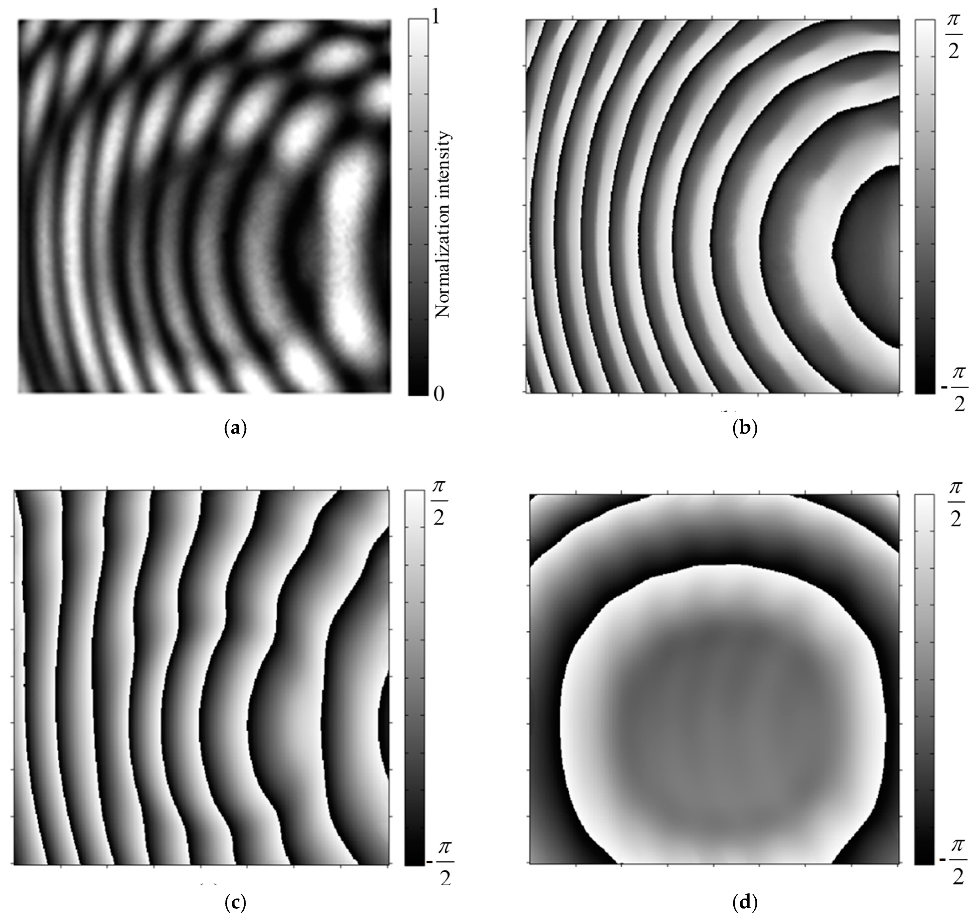
Figure 4a. The light reflected from the reference plate and the interfaces of the tested transparent plate in projected through the beam splitter on the CCD, where the interference field is registered. The example of the field distribution captured by the CCD is shown in Figure 5a.
The tested sample in the experiment was a transparent plate with a thickness approximately 5 mm. The transparent plate was made of JGS1 material and its refractive index was approximately 1.45 at a wavelength of 633 nm. The distance between the reference plate and the front surface H was adjusted to 72.5 mm (M = 10) using a guide rail and adjusting part.
In order to ensure the accuracy and stability of the experiment, the room temperature is stabilized to 25 ± 0.2 ° C . In this paper, we set the phase-shift as δ k = k π 4 ( k = 1 , 2 , 3 ) in Equation (4). The diode laser coupled with the diffraction grating provided the interval of the wavelength change, Δ λ = 3.5 × 1 0 3 nm. The total wavelength-shift and phase-shift used in the experiment were 0.126 nm and 9 π , respectively.
By applying the 36-step algorithm described in Section 2, the information of the front and rear surfaces and thickness variation could be extracted, respectively. The corresponding shapes of the front and rear surfaces of the optical component were calculated after the phase unwrapping had occurred. To remove the high-frequency noise, the phase map was filtered using the windowed Fourier transform (WFT) method [31,32] as shown in Figure 5b–d.
After unwrapping and compensating for the tilt phase aberration of the phase map obtained from the both surfaces of the transparent plate, the profiles of both surfaces of the studied sample can be obtained according to the following relationship:
δ = 4 π d ( x , y ) λ ,
where d describes the optical path difference (OPD). For the three phase maps generated from the reference surface and the front-rear surfaces of the tested transparent plate, ϕ f ( x , y ) , ϕ r ( x , y ) and ϕ f r ( x , y ) can be expressed as follows:
ϕ f ( x , y ) = 4 π [ H ( x , y ) + W f ( x , y ) ] λ ϕ r ( x , y ) = 4 π [ H ( x , y ) + W f ( x , y ) + n 0 ( W r ( x , y ) W f ( x , y ) ) + n 0 T ( x , y ) ] λ ϕ f r ( x , y ) = 4 π [ n 0 T ( x , y ) + n 0 ( W r ( x , y ) W f ( x , y ) ) ] λ
where H represents the distance of the air-gap and W f , W r are front and rear surface profiles of the sample, n 0 and T are the reflective index of the sample, which were assumed to have a uniform distribution, and the thickness of the sample, respectively.
The measured shape of the front surface, rear surface and variation in the thickness are shown in Figure 6a–c, respectively. The mean peak-to-valley (PV) values of the front-and-rear surfaces of the tested transparent plate and its thickness variation were found as 1.38 μm, 0.89 μm and 0.51 μm, respectively, by carrying out 10 repeated measurements at the same position. The repeatability of the 36-step algorithm is confirmed by a pair of measurements taken successively within three days. According to the obtained results by 10 repeated measurements, the root mean square errors (RMSE) for determining both surfaces did not exceed 1.5 nm. The detailed data of the measurements are shown in Table 2. To test the reliability of the 36-step algorithm, the sample was measured by using a ZYGO interferometer (Zygo Corporate, Middlefield, USA), which is considered as a reliable testing instrument in industrial applications. However, it cannot measure the front surface and rear surface profiles simultaneously. Therefore, only one surface was measured, whereas the other surface was covered with Vaseline to suppress its reflection. Then, the other surface was measured while Vaseline covered the first surface. Figure 6b,d,f show the measured front-and-rear surface profiles and variation in the thickness respectively, using a ZYGO interferometer. The results indicate that the shapes measured with the proposed 36-step algorithm were consistent with the ZYGO interferometer. Quantificationally, the PV of front-and-rear surface profiles and variation in the thickness were 1.40 μm, 0.88 μm and 0.53 μm, respectively.

4. Discussion

The previous sections demonstrated the method for separating the superimposed fringe patterns generated as a result of reflection from two parallel surfaces of a tested optical component. The data processing was based on the weighted Fourier transform technique, which is preferable to conventional phase-shifting methods. Despite the previously demonstrated advantages, there are some limitations to this approach. When the phase shift is nonlinear, the phase shift value δm is a function of the phase-shift parameter. The phase shift value of the mth sample can be expressed as
δ m = δ 0 m [ 1 + ε ( δ 0 m ) ] = δ 0 m [ 1 + ε 0 + ε 1 δ 0 m π + ε 2 ( δ 0 m π ) 2 + + ε p ( δ 0 m π ) p ]
where ε is the error coefficient of the phase-shift miscalibration and p is the maximum order of nonlinearity. 
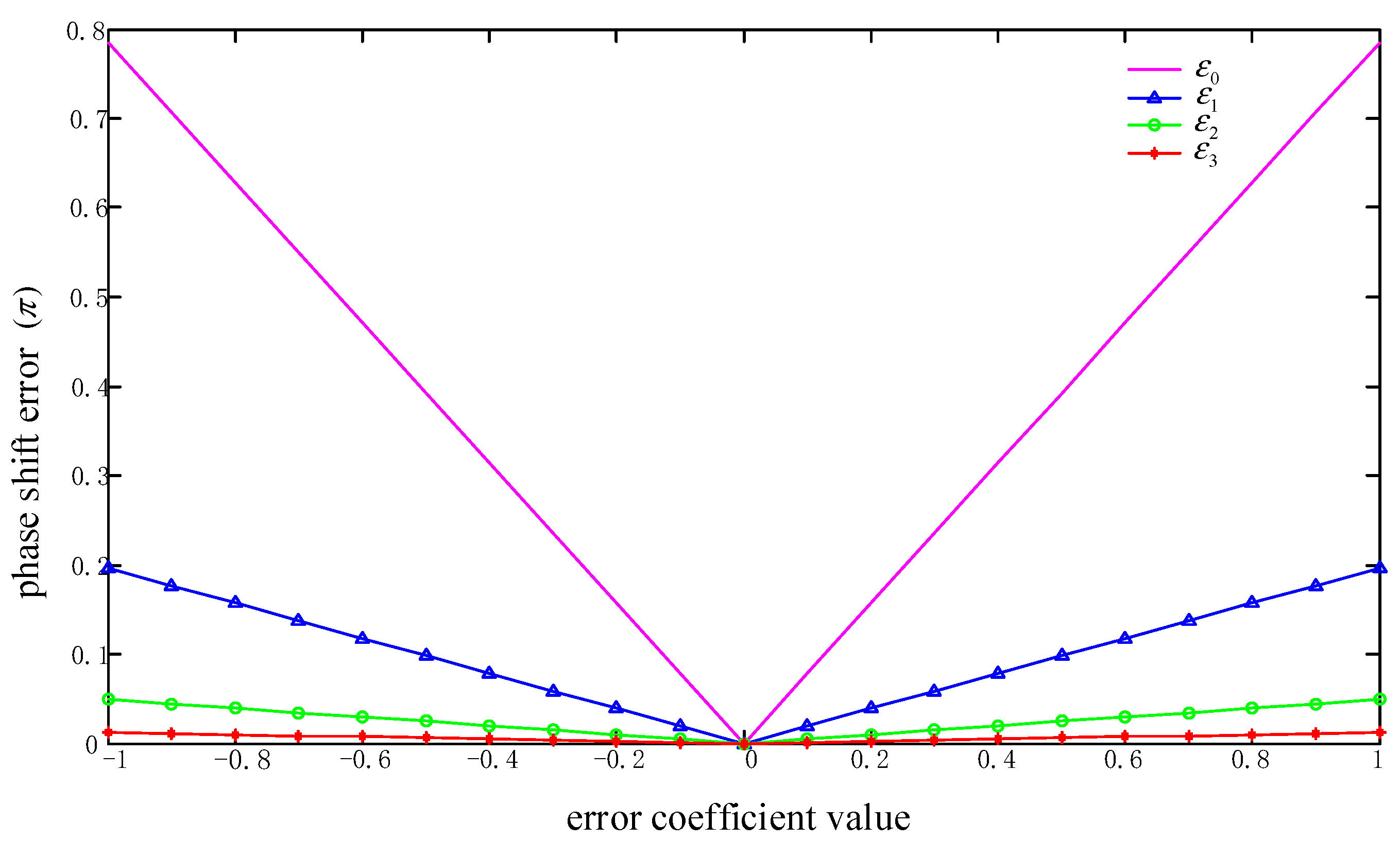
Figure 7 shows the relationship between phase error coefficients of different order ε 0 , ε 1 , ε 2 , ε 3 and the phase shift error. According to this graph, the phase shift error increases with the increase of the coefficient order of the phase-shift error, where the first order linear coefficient ε 0 has the greatest influence and the effects of the second and third nonlinear coefficient order decrease sequentially. In order to reduce the impact of phase-shift error on the accuracy of measurement, it is necessary to suppress the effects of low-order error coefficients, especially the first-order coefficient ε 0 , second-order coefficient ε 1 and third-order coefficient ε 2 .
Further work should focus on improving the phase-insensitive ability to meet the requirement for real-world applications. Adequate results can then be obtained using fewer interferograms.

5. Conclusions

This paper presented a new method for the simultaneous measurement of the front and rear surface profiles of a transparent plate. The simulation analysis and experimental results demonstrated the feasibility of the proposed method. A transparent plate with a thickness of approximately 5 mm was tested as the sample. According to the results, the RMSE using 10 repeat experiments in the determination of both surface profiles did not exceed 1.5 nm. A 36-step algorithm solves the problem regarding the need to restrict the thickness of the sample to a minimum value, for example, more than 5 mm, using the parameters detailed in the paper. This is a good result for a practical measurement application. In addition, a relatively simple experimental setup and reasonably high accuracy are among the advantages of the 36-step algorithm over other techniques [16,19]. Some issues, such as the calculation speed and the cost of a higher quality laser source, must be considered to improve the performance of the 36-step algorithm.

Author Contributions

Writing—Original manuscript Preparation and Software: T.S.; Formal Analysis, Investigation and Methodology: W.Z. and K.Y.; Project Administration, Y.Y.; Supervision: A.K.A.; Review and editing: Y.Y. and S.V.

Funding

The authors gratefully acknowledge the support of the National Science and Technology Major Project (project no. # 2016YFF0101905) and the National Natural Science Foundation of China (NSFC) (no. 51775326).

Acknowledgments

The authors would like to thank Paraskvi Tornari of Institute of Electronic Structure and Laser, Foundation for Research and Technology—Hellas and Wenjing Zhou from department of precision mechanical engineering of Shanghai University for help with this paper.

Conflicts of Interest

The authors declare no conflict of interest.

References

  1. Schmitt, R.; Doerner, D. Measurement technology for the machine integrated determination of form deviations in optical surface. CIPR Ann. Manuf. Technol. 2006, 55, 559–562. [Google Scholar] [CrossRef]
  2. Fang, F.Z.; Zhang, X.D.; Weckenman, A.; Zhang, G.X.; Evans, C. Manufacturing and measurements of freeform optics. CIRP Ann. Manuf. Technol. 2013, 62, 823–846. [Google Scholar] [CrossRef]
  3. Valyukh, S.; Valyukh, I.; Skarp, K. Spectrophotometric determination of reflective liquid crystal cell parameters. J. Appl. Phys. 2006, 99, 8590. [Google Scholar] [CrossRef]
  4. Kim, Y.; Hibino, K.; Sugita, N.; Mitsuishi, M. Absolute optical thickness measurement of transparent plate using excess fraction method and wavelength-tuning Fizeau interferometer. Opt. Express 2015, 23, 4065–4073. [Google Scholar] [CrossRef] [PubMed]
  5. Ishii, M.Y.; Chen, J.; Tsujiuchi, J. Digital phase-measuring interferometry with a tunable laser diode. Opt. Lett. 1987, 12, 233–235. [Google Scholar] [CrossRef] [PubMed]
  6. Takeda, M.; Mutoh, K. Fourier transform profilometry for the automatic measurement of 3-D object shapes. Appl. Opt. 1983, 22, 3977–3982. [Google Scholar] [CrossRef] [PubMed]
  7. Liu, F.W.; Wu, Y.Q.; Wu, F. Phase shifting interferometry from two normalized interferograms with random tilt phase-shift. Opt. Express 2015, 23, 19932–19946. [Google Scholar] [CrossRef] [PubMed]
  8. Su, X.Y.; Dou, Y.F.; Chen, Y.F.; Wang, Y. A flexible fast 3D profilometry based on modulation measurement. Opt. Lasers Eng. 2011, 49, 376–383. [Google Scholar] [CrossRef]
  9. De Groot, P.; Deck, L. Surface profiling by analysis of white-light interferograms in the spatial frequency domain. J. Mod. Opt. 1995, 42, 389–401. [Google Scholar] [CrossRef]
  10. Tsuruta, T.; Ichihara, Y. Accurate measurement of lens thickness by using white-light fringes. J. Appl. Phys. 1975, 14, 369–372. [Google Scholar] [CrossRef]
  11. Kuo; Chuan, W.; Bou, Y.K.; Lai, C.M. Simultaneous measurement of refractive index and thickness of transparent material by dual-beam confocal microscopy. Meas. Sci. Technol. 2013, 24, 075003. [Google Scholar] [CrossRef]
  12. Kim, S.; Na, J.; Kim, M.J.; Lee, B.H. Simultaneous measurement of refractive index and thickness by combining low-coherence interferometry and confocal optics. Opt. Express 2008, 16, 5516–5526. [Google Scholar] [CrossRef] [PubMed]
  13. Liu, K.; Littman, M.G. Novel geometry for single-mode scanning of tunable lasers. Opt. Lett. 1981, 6, 117–118. [Google Scholar] [CrossRef] [PubMed]
  14. Abou Zeid, Y.A.; Wiese, P. Interferometer with a wavelength-tuned diode laser for surface profilemetry. Meas. Sci. 1998, 9, 1105–1110. [Google Scholar] [CrossRef]
  15. Hibino, K.; Oreb, B.F.; Fairman, P.S. Improved algorithms for wavelength scanning interferometry: Application to the simultaneous measurement of surface topography and optical thickness variation in a transparent parallel plate. Proc. SPIE 2002, 177–183. [Google Scholar] [CrossRef]
  16. Okada, K.; Sakuta, H.; Ose, T. Separate measurements of surface shapes and refractive index inhomogeneity of an optical element using tunable-source phase shifting interferometry. Appl. Opt. 1990, 23, 3280–3285. [Google Scholar] [CrossRef] [PubMed]
  17. Yu, Y.J.; Zhang, B.H.; Jiao, Y.F. Phase-shifting algorithm via wavelength tuning based on temporal Fourier transform. Proc. SPIE 2003, 5188, 343. [Google Scholar] [CrossRef]
  18. Hibino, K.; Mitsuishi, M.; Sugita, N.; Hanayama, R.; Kim, Y. Multiple-surface interferometry of highly reflective wafer by wavelength tuning. Opt. Express 2014, 22, 21145–21156. [Google Scholar] [CrossRef]
  19. Deck, L.L. Multiple surface phase shifting interferometry. Proc. SPIE 2001, 424–431. [Google Scholar] [CrossRef]
  20. Kim, Y.; Hibino, K.; Sugita, N.; Mitsuishi, M. Interferometric profile measurement of optical-thickness by wavelength tuning with suppression of spatially uniform error. Opt. Express 2018, 26, 10870–10878. [Google Scholar] [CrossRef]
  21. Hibino, K.; Oreb, B.F.; Fairman, P.S.; Burke, J. Simultaneous measurement of surface shape and variation in optical thickness of a transparent parallel plate in wavelength scanning Fizeau interferometer. Appl. Opt. 2004, 43, 1241–1249. [Google Scholar] [CrossRef] [PubMed]
  22. De Groot, P. Method and System for Profiling Objects Having Multiple Reflective Surfaces using Wavelength Tuning Phase-Shifting Interferometry. U.S. Patent 6 359 692, 19 January 2002. [Google Scholar]
  23. De Groot, P. Measurement of transparent plates with wavelength-tuned phase-shifting interferometry. Appl. Opt. 2000, 39, 2658–2663. [Google Scholar] [CrossRef] [PubMed]
  24. Hibino, K.; Oreb, B.F.; Fairman, P.S. Wavelength-scanning interferometry of a transparent parallel plate with refractive-index dispersion. Appl. Opt. 2003, 42, 3888–3895. [Google Scholar] [CrossRef] [PubMed]
  25. Sun, T.; Zheng, W.W.; Yu, Y.J.; Asundi, A.K.; Valyukh, S. Determination of surface profiles of transparent plates by means of laser interferometry with wavelength tuning. Opt. Lasers Eng. 2019, 115, 59–66. [Google Scholar] [CrossRef]
  26. Kim, Y.; Hibino, K.; Sugita, N.; Mitsuishi, M. Optical thickness measurement of mask blank glass plate by the excess fraction method using wavelength-tuning interferometer. Opt. Lasers Eng. 2013, 51, 1173–1178. [Google Scholar] [CrossRef]
  27. Surrel, Y. Design of algorithms for measurements by the use of phase stepping. Appl. Opt. 1996, 35, 51–60. [Google Scholar] [CrossRef] [PubMed]
  28. Harris, F.J. On the use of windows for harmonic analysis with the discrete Fourier transform. Proc. IEEE 1978, 51–83. [Google Scholar] [CrossRef]
  29. Servin, M.; Estrada, J.C.; Quiroga, J.A. Spectral analysis of phase shifting algorithms. Opt. Express 2009, 17, 16423–16428. [Google Scholar] [CrossRef]
  30. Servin, M.; Estrada, J.C.; Quiroga, J.A. The general theory of phase shifting algorithms. Opt. Express 2009, 17, 21867–21881. [Google Scholar] [CrossRef] [Green Version]
  31. Qian, K.M. Windowed Fourier transform for fringe pattern analysis. Appl. Opt. 2004, 43, 52695–52702. [Google Scholar] [CrossRef]
  32. Qian, K.M. Two-dimensional windowed Fourier transform for fringe pattern analysis: Principles, applications and implementations. Opt. Lasers Eng. 2007, 45, 304–317. [Google Scholar] [CrossRef]
Figure 1. Diagram of the reflected rays forming the interferogram.
Applsci 09 02349 g001
Figure 2. The Hanning window function. (a) Shape of the Hanning window function; (b) evaluating function of the Hanning window in the thickness measurement; (c) evaluating function of the Hanning window in the front-surface measurement; (d) evaluating function of the Hanning window in rear-surface measurement.
Applsci 09 02349 g002
Figure 3. New window function of the 36-step algorithm. (a) Shape of the new window function of the 36-step algorithm defined by w ( 36 ) ; (b) new window function of the 36-step algorithm in the thickness measurement; (c) new window function of the 36-step algorithm in front-surface measurement; (d) new window function of the 36-step algorithm in the rear-surface measurement.
Applsci 09 02349 g003
Figure 4. Experimental setup. (a) Schematic diagram of the interferometer used to measure the profiles of the front and rear surfaces; (b) laboratory photo of the measuring area of the transparent plate in a wavelength-tuning interferometer.
Applsci 09 02349 g004
Figure 5. Distributions of the registered and processed signals obtained in the experiment. (a) The fringe pattern from both surfaces of the transparent plate at the initial wavelength; (b) wrapped phase map of the front surface after the windowed Fourier transform (WFT) filter was applied; (c) wrapped phase map of the rear surface after the WFT filter was applied; (d) wrapped phase map of variation in the thickness after the WFT filter was applied.
Applsci 09 02349 g005
Figure 6. The surface profiles measured with the 36-step algorithm and the ZYGO interferometer. (a) The profile of the front surface obtained with the 36-step algorithm; (b) the profile of the front surface obtained the ZYGO interferometer; (c) the profile of the rear surface obtained with the 36-step algorithm; (d) the profile of the rear surface obtained with the ZYGO interferometer; (e) the profile of the variation in the thickness obtained with the 36-step algorithm; (f) the profile of variation in the thickness obtained with the ZYGO interferometer.
Applsci 09 02349 g006
Figure 7. Relationship between phase error coefficients of different order and phase shift error.
Applsci 09 02349 g007
Table 1. Frequency information of each measuring surface.
No. v n / v 1 Remark
v 1 1thickness
v 2 MFront interface
v 3 M + 1Rear interface
Table 2. The result of the peak-to-valley (PV) value of three surfaces obtained by 10 repeated measurements using the 36-step algorithm (μm).
Measurement NumberAverage ValueRMSE
12345678910
front surface1.38151.38091.38141.38241.38151.38031.38141.38381.38101.38021.38140.0010
rear surface0.89320.89230.89430.89150.89240.89110.89320.89270.89000.89110.89220.0013
variation of thickness0.51140.51260.50150.51270.51130.51120.51030.51390.51170.51080.51160.0011

