Measurement System of Metal Magnetic Memory Method Signals around Rectangular Defects of a Ferromagnetic Pipe

Abstract

Oil and gas pipeline networks require the periodic inspection of their infrastructure, which can cause gas and oil leakage with several damages to the environment and human health. For this, non-destructive testing (NDT) techniques of low-cost and easy implementation are required. An option is the metal magnetic memory (MMM) method, which could be used for real-time monitoring defects of ferromagnetic structures based on the analysis of self-magnetic leakage fields distribution around each defect. This method only requires magnetic sensors with high resolution and a data processing system. We present a measurement system of tangential and normal MMM signals of three rectangular defects of an ASTM A-36 steel pipe. This system is formed by a magnetoresistive sensor, an Arduino nano and a virtual instrumentation. The measured magnetic signals have non-uniform distributions around the rectangular defects, which have small differences with respect to the results obtained of a 2D magnetic dipole model. The size of each rectangular defect is related to the amplitude and shape of its tangential and normal MMM signals. The proposed system could be used for real-time monitoring of the size and location of rectangular defects of ferromagnetic pipes. This system does not require expensive equipment, operators with high skill level or a special treatment of the ferromagnetic samples.

1. Introduction

The infrastructure for a gas and oil pipeline network must be constantly monitored using non-destructive testing (NDT) techniques to assure its safe operation. Pipeline faults can cause oil and gas leakage with severe damages in the environment and human health [1,2]. The pipeline network safety is a priority in the gas and oil industries, which require low-cost NDT techniques for real-time monitoring of defects and flaws in the pipeline. Thus, the pipeline network requires periodic inspections and suitable maintenances that avoid future accidents. Generally, in these inspections conventional NDT techniques are used, such as infrared thermography testing, radiographic testing, visual testing, ultrasonic testing, acoustic emission, liquid penetrant testing and Eddy current testing [3,4,5,6]. Liquid penetrant testing is useful for inspection of surface defects in ferromagnetic samples, although these defects should be contaminants free [7]. On the other hand, ultrasonic testing has high sensitivity for detection of small flaws, but it needs reference standards for calibrating the equipment as well as operators with extensive training and experience [8,9]. Another NDT technique is the acoustic emission, which is used for monitoring discontinuities on a large area using multiple sensors whose signals must be interpreted by inspectors with extensive technical knowledge [10]. Infrared thermography is another NDT technique that has high sensitivity to temperature variations and it needs expensive equipment [5]. Also, radiographic testing has a high sensitivity for detecting flaws. Nevertheless, this technique presents limitations such as radiation hazard and highly expensive equipment, and it requires operators with high skill level [10,11,12]. Finally, Eddy current testing is employed for inspection of defects based on electromagnetic induction [12,13]. However, this technique needs an external magnetic field source to induce Eddy currents.

Recently, several studies about the defects inspection of ferromagnetic structures have been reported using the metal magnetic memory (MMM) method [14,15,16,17,18,19,20,21]. The MMM method is a passive magnetic testing technique, which is different to the conventional magnetic flux leakage method. This MMM method may be used for monitoring defects or degrees of stress concentration in ferromagnetic materials measuring their spontaneous surface micro-magnetic signals [20,21]. These signals can be affected by several factors such as different manufacture processes applied to the ferromagnetic materials, considering types of heat treatment, welding, casting and forging [22]. This method could be employed for monitoring defects of ferromagnetic structures based on the analysis of self-magnetic leakage fields distribution around each defect. The MMM method does not require additional equipment, external magnetic field sources and special treatment on the structures surface. Thus, this magnetic method has a simple operation principle and it could be used for defects inspection of pipeline network using magnetic sensors with high resolution. However, more studies related to this method are necessary to predict the relation between the defect size (depth and width) and variations of the amplitude and shape of the MMM signals. In order to study this relation, we measure the tangential and normal MMM response around three different rectangular defects on the external surface of a ferromagnetic pipe (ASTM A-36 steel) using a simple measurement system. This system uses a low-cost magnetoresistive sensor, an Arduino nano and a virtual instrumentation. In addition, it can be used without special equipment, additional treatment on the surface of ferromagnetic pipes or operators with high skill level. The proposed system could be employed for real-time monitoring of the size and location of rectangular defects on the external surface of ferromagnetic pipes.

This paper consists of the following sections. Section 2 includes the analytical response of tangential and normal MMM signals of rectangular defects. Section 3 presents the measurement system and experimental results of the tangential and normal MMM signals of three different rectangular detects of a ferromagnetic pipe. Section 4 summarizes the conclusions and outlines future research works.

2. Analytical Model of the MMM Signals

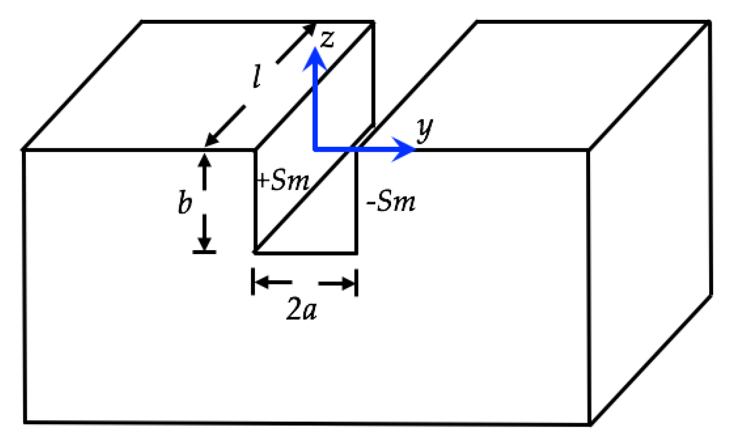
This section describes the MMM signals of a rectangular defect of a ferromagnetic material considering the 2D magnetic dipole model. Figure 1 shows a rectangular defect that contains 2a width, b depth and a magnetic charge density ± Sm around the defect edges. A 2D magnetic dipole model is employed to predict MMM signals around the rectangular defect. This model can determine the MMM signals of defects with simple geometries [23,24]. Forster [25,26,27] developed a theoretical modeling and experimentation of the MMM signals of discontinuities on test specimens. In addition, Zatsepin and Schcerbinin [28,29] proposed analytical models for the tangential and normal MMM signals around a 2D rectangular defect, considering a constant pole density on its surfaces. These models were modified by Edwards and Palmer [30] to evaluate the magnetic field (S_m) inside the gap of a rectangular defect. Thus, the tangential (Hy) and normal (Hz) MMM signals for a rectangular defect on a ferromagnetic pipe can be calculated by [27,28]:

$$H_y=\frac{H_{\mathrm{o}}\pi n\left(\mu -1\right)}{2{\tan }^{-1}n\left(n+\mu \right)}\{{\tan }^{-1}\left(\frac{b\left(y+a\right)}{{\left(y+a\right)}^2+z\left(z+b\right)}\right)-{\tan }^{-1}\left(\frac{b\left(y-a\right)}{{\left(y-a\right)}^2+z\left(z+b\right)}\right)\}$$

(1)

$$H_z=\frac{H_0\pi n\left(\mu -1\right)}{4{\tan }^{-1}n\left(n+\mu \right)}\ln \left\{\frac{\left[{\left(y+a\right)}^2+{\left(z+b\right)}^2\right]\left[{\left(y-a\right)}^2+z^2\right]}{\left[{\left(y+a\right)}^2+{\left(z\right)}^2\right]\left[{\left(y-a\right)}^2+{\left(z+b\right)}^2\right]}\right\}$$

(2)

where n = b/a, H₀ is the uniform magnetic field along the y-axis (i.e., axial axis) of the ferromagnetic pipe, b and 2a are the depth and width of the rectangular defect, respectively, y and z are the horizontal and vertical axes, respectively, and µ is the relative permeability of the material.

The magnetic field density inside the defect (S_m) was determined by Edwards and Palmer [30] as:

$$S_m=\frac{{\mu }_0\mu H_0\pi n\left(\mu -1\right)}{{\tan }^{-1}n\left(n+\mu \right)}$$

(3)

where µ₀ is the magnetic permeability of free space.

Equations (1)–(3) consider a small size for each rectangular defect in comparison with the diameter of the pipe (i.e., the curvature of the pipe wall is neglected). Figure 2 depicts the behaviour of the tangential (Hz) and normal (Hy) MMM signals of a rectangular defect on a ferromagnetic sample using Equations (1) and (2). For this case, we use the following data: µ = 180, H₀ = 0.7958 A/m, a = 2.25 mm and b = 3.5 mm. For Hz component, the maximum value occurs at the defect center. With respect to the Hy component, it presents a zero value at the defect center and two peaks with maximum and minimum values on both sides of the rectangular defect.

3. Results and Discussion

In this section, the MMM signals of three different rectangular defects of an ASTM A-36 steel pipe are presented. This pipe has the following dimensions: 247.0 mm length, 48.06 mm outer diameter and 3.65 mm thickness.

Figure 3 shows the measurement system of MMM signals around three different rectangular defects of an ASTM A-36 steel pipe. This system includes a rotatory mechanism, a magnetoresistive sensor (MAG3110), an Arduino nano (ATmega328) and a virtual instrumentation developed in Delphi Borland code [31]. The rotatory mechanism uses a motor (Bühler GmbH, Braunschweig, Germany) that is supplied with 1.5 V dc to generate a rotational motion of 2 rpm. The measurement system is fabricated of non-magnetic materials such as nilamide and aluminium, which do not affect the self-magnetic leakage flux of the ferromagnetic pipe. The pipe sample is collocated in the rotatory supports, keeping a constant distance of 2 mm between the external surface of the pipe and the magnetoresistive sensor. The pipe has three rectangular defects with different depth and width along its length. These defects (see Figure 4) have the following dimensions: S1 (4.36 mm width and 3.65 mm depth), S2 (3.80 mm width and 2.0 mm depth) and S3 (2.80 mm width and 0.50 mm depth). The tangential and normal MMM signals around the three defects are measured using the magnetoresistive sensor. The sensor has a resolution of 30 nT, a sensibility of 100 nT, and it uses an I²C interface to communicate with Arduino nano (ATmega328). The measured MMM signals of the three defects are processed using a virtual instrumentation, which is developed in Delphi Borland code [31]. For the analytical model, values of H₀ for each defect are determined to estimate the best fit of Equations (1)–(3) for the corresponding experimental data. For these cases, we assumed a relative permeability of 180.

Figure 5 depicts the tangential MMM signal of the first rectangular defect (S1), which is obtained using the analytical model and proposed measurement system. The measured tangential MMM signal exhibits a peak (173.2 µT) at the defect center (y = 0 mm). This peak corresponds with the maximum depth (3.65 mm) of the defect S1. This peak width is related to the defect width (4.36 mm). The width of the measured tangential MMM signal is less than the signal of the analytical model. This difference can occur because the 2D magnetic dipole method considers a constant magnetic permeability of the ferromagnetic sample. In the positions from −5.0 mm to 5.0 mm, the analytical tangential MMM signal has a high absolute difference (18.52 µT and 47.18 µT) with respect to the measured MMM signal. On the other hand, the normal MMM signal of defect S1 has two peaks (112.2 µT and −143.6 µT) close to both edges of the defect S1 (see Figure 6). These two peaks represent a change in the polarity of the normal MMM signal due to different polarities of the magnetic charges on the defect edges, in which the normal MMM signal reached a value zero at the defect center (y = 0 mm). The distance along y-axis between the two peaks values is related to the defect width (4.36 mm). The maximum and minimum magnitudes of the normal MMM signal are achieved along the positions close to ±2.0 mm. The normal MMM signal registers a magnetic flux offset about ±80.0 µT. For this case, the normal MMM signal obtained through analytical model has a good approximation in comparison with the measured MMM signal. In the positions from −5.0 mm to 5.0 mm, these signals have an absolute difference of 8.22 µT and 24.52 µT, respectively.

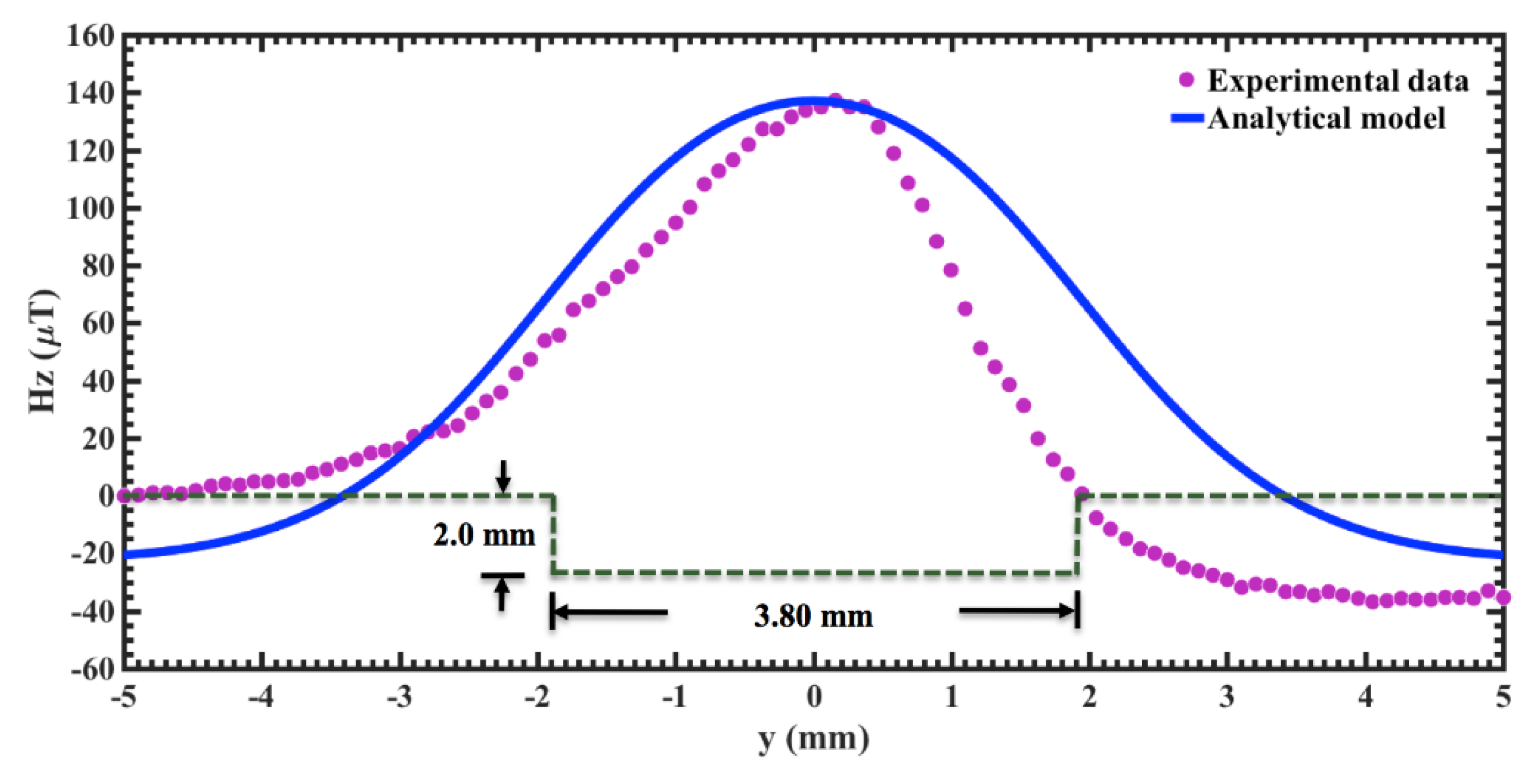
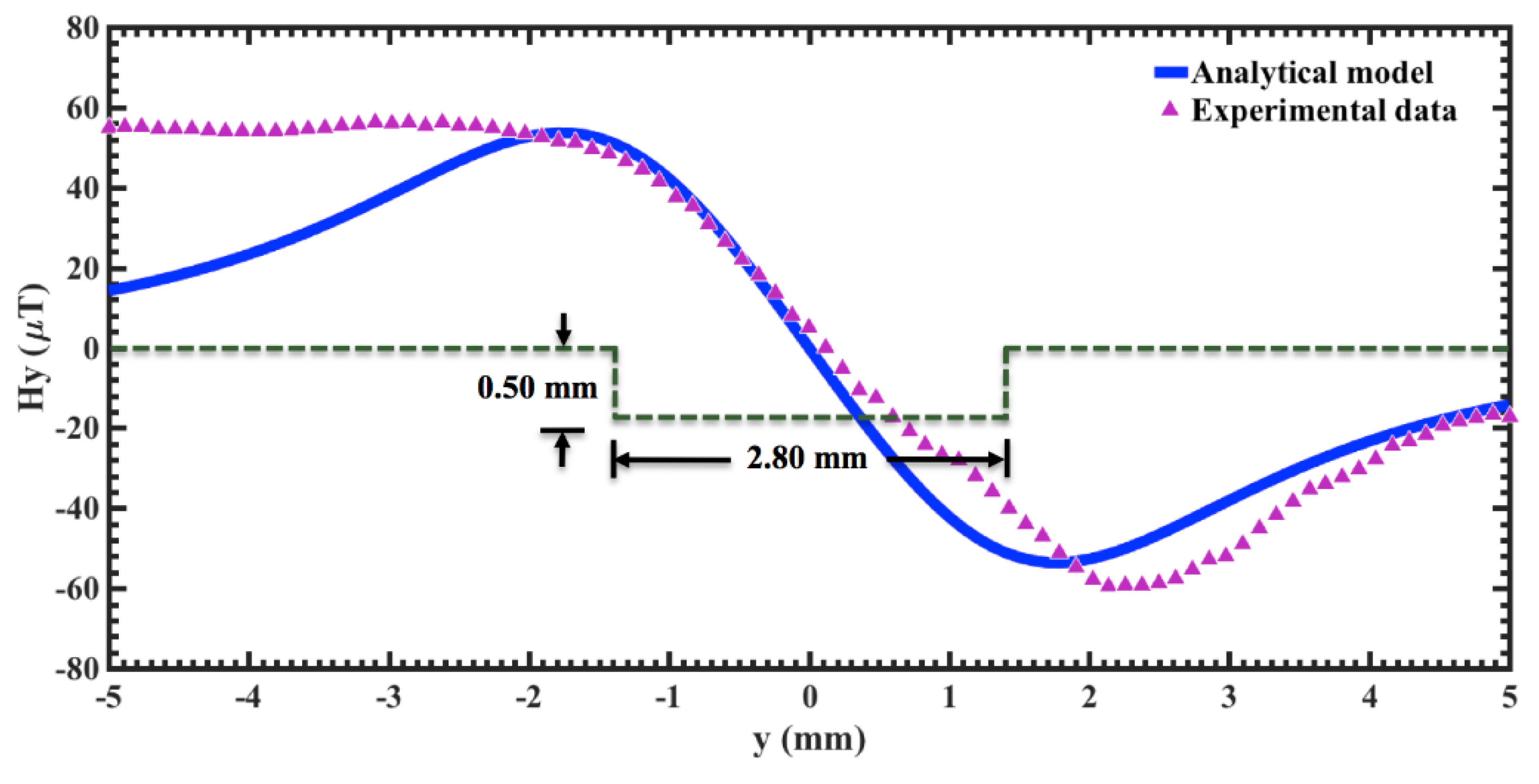
Figure 7 shows the measured tangential MMM signal of the second rectangular defect (S2). This MMM signal has a maximum value (137.1 µT) at the defect center. This value is 36.1 µT less than the maximum field of the defect S1, which represents a reduction of 20.8%. This decrease is related to the less depth (2.0 mm) of the defect S2 in comparison to the depth (3.65 mm) of defect S1. The width of the tangential MMM signal is related to the defect width (3.80 mm). The measured tangential MMM response has a magnetic flux offset close to 35 µT at the right edge of the defect S2. The measured tangential MMM signal has a behaviour similar to that obtained by the analytical model. On the other hand, the measured normal MMM signal (see Figure 8) of the defect S2 has maximum and minimum values (25.8 µT and −27.2 µT) around both defect edges. The polarity of this MMM signal is altered at the defect center S2 (y = 0 mm). In addition, the normal MMM signal obtained through the analytical model agree well with the experimental data in the positions between −2.0 and 2.0 mm. However, the analytical response of the tangential MMM signal has a high absolute difference (18.67 µT and 20.17 µT) with respect to the measured MMM signal in the positions from −5.0 m to 5.0 mm. The offset of both tangential and normal MMM signals is due to the magnetic flux along the pipe surface close to the defects. In addition, the results of both MMM signals determined with the 2D magnetic dipole method have a discrepancy with respect to measured MMM responses. This is due to the fact that the analytical model considers a constant magnetic permeability of the ferromagnetic material. In addition, the defect S2 has edges with small inclinations that can affect the measured response of both MMM signals.

For the third rectangular defect (S3), the measured tangential MMM signal has a maximum value (53.6 µT) at the defect center (see Figure 9). This value is 119.6 µT less than that obtained of the defect S1, which represents a reduction of 69.1%. This largest variation is related to the smallest depth (0.50 mm) of the defect S3. In addition, the width of this tangential MMM response decreases in comparison to the MMM signal of the defects S1 and S2, respectively. For the defect S3, both tangential MMM signals have a similar behaviour between the positions from −1.4 mm to 1.4 mm. The distance between these positions corresponds to the width of the defect S3. Nevertheless, the absolute difference between both MMM signals increases for positions out of this width. For y = ±5.0 mm, the absolute difference between both tangential MMM signals are 8.12 µT and 20.68 µT, respectively. On the other hand, the normal MMM response of the defect S3 has two peaks values (48.3 µT and −59.5 µT) close to their edges, achieving a polarity shift at the defect center (see Figure 10). The defect S3 has less width (2.80 mm) in comparison to the defects S2 (3.80 mm) and S3 (4.36 mm), respectively, which causes a reduction in the width of the tangential MMM signal. In addition, the maximum and minimum magnitudes (48.3 µT and −59.5 µT) of the measured normal MMM signal reach close to the edges of the defect S3. For the positions between −1.4 mm and 1.4 mm, the analytical normal MMM signal has a good approximation with respect to the measured MMM signal. However, the absolute difference between these signals increases for positions out of the range y = ± 1.4 mm. For the positions y = ± 5.0 mm, the absolute difference between both normal MMM signals are 40.69 µT and 8.12 µT, respectively. The ideal approximation of the analytical model is the main reason for the differences between measured signals values and the analytical model-predicted ones. For instance, the analytical model considers a constant magnetic permeability of the ferromagnetic material. In addition, this analytical model is suitable for defects with a completely rectangular shape. In the real defect, the shape is approximately rectangular with small inclinations along its edges. Also, the analytical model does consider a uniform distribution of both MMM signals around each defect.

The defect edges generate two peaks in the shape of the normal MMM signals, which indicate a polarity shift of the magnetic flux at the defect center. The defect with the largest depth achieves the highest value of the tangential MMM response, while the defect with smallest depth has the lowest value of tangential MMM signal. Thus, these parameters could be employed to predict the size (depth and width) and location of rectangular defects of ferromagnetic pipes using the MMM method. The measurement system could be used for real-time monitoring of rectangular defects on ferromagnetic pipes. This system does not require special treatment of the ferromagnetic sample, complex equipment and operators with extensive training. In comparison with other NDT techniques such as the Eddy current testing and magnetic flux leakage testing, the MMM method does not need to apply external magnetic field on the ferromagnetic pipe. It allows the decrease of additional equipment and special treatment on the pipe surface. On the other hand, the X-ray testing is an NDT that uses expensive equipment and operators with extensive technique experience. Another NDT testing is liquid penetrant inspection, which has low cost, but it can only detect surface flaws. In addition, it requires pipe surfaces free of contaminants. The MMM method could be integrated with other NDT testing such as electrical resistance measurement and acoustic emission technique. For instance, the comparison of analysis related to the electrical resistance monitoring and acoustic emission technique could be used in the assessment of damage and defects in structures [32,33,34,35]. For structures formed with ferromagnetic materials, the results of both techniques could be used with those obtained through MMM method for monitoring the location, dimensions and shape of their defects. Thus, these NDT tests could be complementary for inspection of damages in structures with ferromagnetic materials.

4. Conclusions

A measurement system for real-time monitoring of the rectangular surface defects of ferromagnetic pipes is reported. This system detects the variations of the tangential and normal MMM signals around the defects, which could be used to determine their location and size. The proposed system uses a low-cost magnetoresistive sensor, an Arduino nano and a virtual instrumentation. This system could allow the inspection of rectangular defects and it does not need expensive equipment and operators with extensive experience. The size (depth and width) of the defects is related to the amplitude and shape of these magnetic signals. The measured MMM signals have non-uniform distributions, which registered differences with respect those calculated through a 2D magnetic dipole model. These differences were caused by small inclinations along the edges of the three rectangular defects. In addition, the analytical model considered a constant magnetic permeability of the ferromagnetic pipe.

Future studies will include the analysis of MMM signals around small defects with different shapes (e.g., triangular, cylindrical and spherical shape) on the surface of ferromagnetic pipes. In addition, we will study the relations between size and shape of the defects with respect to the shifts in their measured MMM signals.