Prediction of Ultimate Axial Capacity of Square Concrete-Filled Steel Tubular Short Columns Using a Hybrid Intelligent Algorithm

Abstract

It is crucial to study the axial compression behavior of concrete-filled steel tubular (CFST) columns to ensure the safe operation of engineering structures. The restriction between steel tubular and core concrete in CFSTs is complex and the relationship between geometric and material properties and axial compression behavior is highly nonlinear. These challenges have prompted the use of soft computing methods to predict the ultimate bearing capacity (abbreviated as N_u) under axial compression. Taking the square CFST short column as an example, a mass of experimental data is obtained through axial compression tests. Combined with support vector machine (SVM) and particle swarm optimization (PSO), this paper presents a new method termed PSVM (SVM optimized by PSO) for N_u value prediction. The nonlinear relationship in N_u value prediction is efficiently represented by SVM, and PSO is used to select the model parameters of SVM. The experimental dataset is utilized to verify the reliability of the PSVM model, and the prediction performance of PSVM is compared with that of traditional design methods and other benchmark models. The proposed PSVM model provides a better prediction of the ultimate axial capacity of square CFST short columns. As such, PSVM is an efficient alternative method other than empirical and theoretical formulas.

1. Introduction

Concrete-filled steel tubular (CFST) refers to the composite member formed by filling steel tubular with concrete. CFST makes use of the interaction between concrete and steel tubular under stress to give full play to the advantages of both materials, that is, it not only greatly improves the plasticity and toughness of concrete, but also can avoid or delay the local buckling of steel tubular. CFST has the characteristics of high bearing capacity, good plasticity and toughness, convenient construction, and excellent seismic and refractory performance [1]. Therefore, CFST structures are widely used at home and abroad, of which an important type is the CFST column. CFST columns are mainly divided into square and circular CFST columns based on different sectional forms. Square CFST columns are easy to process and have better stability. Since they are mostly subjected to axial compression, it is necessary to study the ultimate axial capacity of square CFST columns [2].

At present, many experimental studies have been carried out on the mechanical properties of CFST columns under axial compression. Giakoumelis et al. [3] presented the behavior of circular CFSTs with various concrete strengths under axial load, and examined the effects of several factors. Evirgen et al. [4] adopted 16 hollow cold-formed steel tubulars and 48 CFSTs for axial compression tests, and investigated the effects of width/thickness ratio, concrete strength, and geometrical shape of specimens on ultimate loads. The efficient and accurate numerical simulation techniques developed rapidly [5], which were combined with axial compression tests, and fruitful results have been achieved. Tao et al. [6] and Han et al. [7] respectively established a finite element model considering material nonlinearity and interaction between concrete and steel tubular, and verified the model with experimental data. Lyu et al. [8] analyzed the ultimate bearing capacity, failure mode, and load-displacement curve of square thin-walled CFST short columns with reinforcement stiffener at different temperatures using comparative experiments and ABAQUS simulation. Briefly, the ultimate axial capacity is an essential mechanical index to evaluate the performance of CFST columns under axial compression in both laboratory experiments and numerical simulations [9,10]. However, axial compression tests are time-consuming and laborious. It is also difficult to consider all of the complicated conditions and material properties in numerical simulations. For these purposes, scholars have always been exploring alternative soft computing methods to conveniently acquire the accurate ultimate axial capacity.

Mass experimental data have been produced by previous studies, that provide a data basis for mathematical modeling to estimate the ultimate axial capacity of CFST columns. Lu et al. [11] studied the calculation method for ultimate axial capacity of square CFST short columns considering size effect. The calculation formulas in the present codes of different countries were revised by collecting many experimental results. Yu et al. [12] developed a simplified statistical method based on 663 tests to predict the ultimate strength of circular CFST columns under concentric load. The confinement effect on the concrete and the influence of relative slenderness were taken into account. Other simplified calculation methods have also been proposed. For example, a simple method using an equivalent slenderness ratio was suggested by Zheng et al. [13] to calculate the load-bearing capacity of CFST laced columns. None of the above-proposed methods have been extensively used due to the limitations of application scope. It is imperative to develop a general and precise method for calculating the ultimate axial capacity.

In recent years, with the rapid development of artificial intelligence techniques, machine learning algorithms (MLAs) have been popularized in all walks of life [14]. By virtue of the excellent nonlinear learning ability, MLAs have already been employed to calculate the ultimate axial capacity of CFSTs. Artificial neural networks (ANN) have become the most commonly used MLA. Saadoon et al. [15] utilized ANN to develop a model for predicting the ultimate strength of rectangular CFST beam-columns under eccentric axial loads. They used the same method to model and predict the ultimate strength of circular CFST beam-columns [16]. The predicted values were more accurate than the AISC and EC4 values in both cases. Similarly, ANN was applied in [17,18,19]. In addition, Moon et al. [20] presented an alternative method to determine the confinement effect of the concrete infill and the axial load capacity of the stub CFST by using fuzzy logic. The focus was made on the accurate estimation of the confinement effect of the CFST using the fuzzy-based model. Güneyisi et al. [21,22] respectively proposed a new formulation for the axial load carrying capacity of circular CFST short columns and concrete-filled double skin steel tubular composite columns based on gene expression programming (GEP). The GEP model was much better than the available formulae, yielding a higher correlation coefficient and lower error. MLAs were also used to estimate other properties of CFSTs. Al-Khaleefi et al. [23] and Wang et al. [24] each predicted the fire resistance and load-strain relationship of CFSTs with different dimensions and parameters using ANN. The prediction model for the ultimate pure bending moment of CFSTs via adaptive neuro-fuzzy inference system was raised by Basarir et al. [25].

The application of MLAs in CFST performance index calculation is still in its infancy. To the best of our knowledge, some advanced algorithms such as support vector machine (SVM) [26] have not been applied in this field until now. SVM is a new supervised learning method developed in statistical learning theory that performs well in solving small sample, nonlinear, and high dimensional problems [27]. To date, SVM has been widely used in various fields of structural engineering, including dam safety, scour monitoring, civil architecture, etc., due to its potential in nonlinear regression, function approximation, and pattern recognition [28,29,30,31]. In brief, SVM can effectively deal with the data modeling problem under the condition of limited samples because of superior generalization ability and dimensionality insensitivity [32]. Nevertheless, the adjustment and optimization of SVM parameters is an essential problem, which greatly influences prediction effects. The metaheuristic algorithm does not depend too much on the organization structure information of the algorithm, which is suitable for parameter optimization and function calculation. Particle swarm optimization (PSO) is a global random search algorithm based on swarm intelligence [33]. PSO is easier to implement and produces more accurate results than other optimization algorithms, such as genetic algorithm (GA) [34]. In this paper, given enough experimental data of axial compression tests for square CFST short columns, a combined model termed PSVM (SVM optimized by PSO) is proposed to predict the ultimate axial capacity. The prediction performance of PSVM is verified by an independent test set and multi-model comparison. Performance assessment results are quantified by evaluation criteria. The simulation results show the feasibility and superiority of the proposed PSVM model.

The rest of the paper is organized as follows. In Section 2, the axial pressure test procedure and dataset compilation are briefly described. The mathematical principles of SVM and PSO are presented in Section 3. Section 4 expatiates the complete implementation of PSVM. Section 5 illustrates and discusses the results of model validation and sensitivity analysis, and depicts a prediction error correction method. Conclusions and perspectives are finally provided in Section 6.

2. Experimental Dataset Construction

Dataset construction is the first step in modeling prediction. Axial compression tests are carried out on short columns with different geometric sizes and material properties, and 180 groups of experimental data are obtained. The dataset lays a foundation for N_u value prediction using soft computing methods.

2.1. Axial Compression Test

To ensure the richness and diversity of experimental data, 180 specimens of different specifications were designed by changing the geometric, steel and concrete properties of square CFST short columns. Three specimens of each specification were made to reduce the influence of the dispersion of axial compression test data, and a total of over 540 specimens were made. Before performing a series of axial compression tests, the multi-mechanical properties of steel and concrete in CFST specimens of different specifications were measured based on GB/T 228.1-2010 and GB/T 50081-2002, respectively.

The test consists of five main steps: (1) design of specimens; (2) selection and preliminary processing of steel tube; (3) selection and production of concrete mix; (4) pouring and curing of specimens; (5) loading and measurement. The axial compression tests of all specimens were performed on a hydraulic loading system with sufficient loading force. The schematic diagram of the experimental device is shown in Figure 1. A cushion plate is placed between the specimen and loading plate to ensure that the CFST specimen is under uniform stress during loading. The preloading should be carried out before the formal loading, and all specimens should bear the central load. The preloading force cannot exceed 30% of the expected ultimate axial capacity. The multi-stage loading was adopted in the test process [35,36] and the automatic data acquisition system was employed to record the axial load until the specimen failure. After the completion of all tests, the arithmetic mean of the ultimate axial capacity of the three specimens of each specification was taken as the final ultimate axial capacity N_u.

2.2. Input Selection and Dataset Compilation

In addition to the output variable N_u through multiple tests, the model input variables need to be determined for experimental dataset construction. Seven input variables (D,t,L,f_y,E_s,f_c,E_c) were identified according to different expressions from current codes of GJB 4142-2000 (see Equation (1)), AIJ 1997 (see Equation (2)), AISC-LRFD 1999 (see Equation (3)), and EC4 2004 (see Equation (4)) [37], which are marked in Figure 1 and described in

Table 1. Statistics of model input and output variables.

Direction	Category	Symbol	Description	Minimum	Maximum	Mean
Input	Geometric properties	D (mm)	Side length of the square section	100.00	323.00	152.88
		t (mm)	Thickness of the steel tubular	1.44	7.47	4.13
		L (mm)	Length of the specimen	300.00	969.00	466.53
	Steel properties	fy (MPa)	Yield strength of steel	198.00	835.00	340.83
		Es (MPa)	Elasticity modulus of the steel	180,518.00	214,000.00	202,273.54
	Concrete properties	fc (MPa)	Compressive strength of the core concrete	10.65	91.10	45.79
		Ec (MPa)	Elasticity modulus of the core concrete	23,528.00	42,600.00	30,928.75
Output	Dependent variable	Nu (kN)	Ultimate bearing capacity of the specimen under axial compression	507.00	5873.00	1978.91

. Specifically, the first five variables (D,t,L,f_y,f_c) were selected based on Equations (1) and (2). $E_s$ and $E_c$ were then selected as input variables since both ${\lambda }_c$ in Equation (3) and $\chi$ in Equation (4) are related to them. These seven selected variables include geometric, steel, and concrete properties, which can represent most features of CFST specimens of a certain specification. A total of 180 groups of data were ultimately compiled into a complete experimental dataset, and the descriptive statistics of model input and output variables are shown in Table 1.

$$N_u=(1.18+0.85\frac{f_y{A}_s}{f_c{A}_c})f_c{A}_{sc},$$

(1)

$$N_u=0.85f_c{A}_c+f_y{A}_s,$$

(2)

$$N_u=\{\begin{array}{l}{0.658}^{{\lambda }_c{}^2}{F}_{my}{A}_s,{\lambda }_c\le 1.5\\ \frac{0.877F_{my}{A}_s}{{\lambda }_c{}^2},{\lambda }_c>1.5\end{array},$$

(3)

$$N_u=\chi (f_c{A}_c+f_y{A}_s),$$

(4)

where $f_y$ is the yield strength of steel, $f_c$ is the compressive strength of the core concrete,$A_s,A_c,A_{sc}$ are respectively the cross section area of the steel tubular, core concrete, and CFST, ${\lambda }_c$ is the relative slenderness ratio, $F_{my}$ is the modified yield strength of steel, and $\chi$ is the axial stability factor.

3. Soft Computing Methodologies

The PSVM model based on the combination of SVM and PSO is presented for N_u value prediction. Several common indexes and a comprehensive index are used to measure the prediction performance of PSVM and other benchmark models.

3.1. Support Vector Machine

The basic idea of SVM is to map the nonlinear problem from low-dimensional to high-dimensional spaces by using the kernel function, thereby solving the nonlinear problem by the linear method [38]. Given $N$ sample datasets $\left\{({\mathit{x}}_i,y_i),i=1,2,\cdots ,N\right\}$, ${\mathit{x}}_i=[x_{1i},x_{2i},\cdots ,x_{ni}]\in {ℝ}^{n_l}$ is the input data, and $y_i\in {ℝ}^{n_h}$ is the output data corresponding to ${\mathit{x}}_i$. A nonlinear mapping $\phi (\mathit{x}):{ℝ}^{n_l}\to {ℝ}^{n_h}$ is used to map the input data ${\mathit{x}}_i$ into a high-dimensional feature space ${ℝ}^{n_h}$, where a linear function $f(\mathit{x})$ exists to describe the nonlinear relationship between input and output. The linear function $f(\mathit{x})={\mathit{\omega }}^T\phi (\mathit{x})+b$ is exactly the regression function of SVM, where $\mathit{\omega }$ is the weight vector, and $b$ is the offset.

To reduce the error between training data and ε-insensitive loss function, SVM minimizes the structural risk. The formula is as follows:

$$\underset{\mathit{\omega },b}{\min }\frac{1}{2}{\Vert \mathit{\omega }\Vert }^2+C{\displaystyle \sum _{i=1}^N\max (0,\left|y_i-{\mathit{\omega }}^T\phi ({\mathit{x}}_i)-b\right|-\epsilon )},$$

(5)

where $\epsilon$ is the insensitive loss coefficient, and $C,C>0$ is the penalty factor.

After introducing the slack variables ${\xi }_i$ and ${\xi }_i{}^{*}$, Equation (5) is transformed into the following optimization problem with constraints.

$$\begin{array}{l}\underset{\mathit{\omega },b}{\min }\left[\frac{1}{2}{\Vert \mathit{\omega }\Vert }^2+C{\displaystyle \sum _{i=1}^N({\xi }_i+{\xi }_i{}^{*})}\right]\\ s.t.\{\begin{array}{l}{y}_i-[{\mathit{\omega }}^T\phi ({\mathit{x}}_i)+b]\le \epsilon +{\xi }_i\\ {\mathit{\omega }}^T\phi ({\mathit{x}}_i)+b-y_i\le \epsilon +{\xi }_i{}^{*}\\ {\xi }_i,{\xi }_i{}^{*}\ge 0,i=1,2,\cdots ,N\end{array}\end{array}$$

(6)

By establishing the Lagrangian function and satisfying the Karush–Kuhn–Tucker conditions, Equation (6) is regarded as a quadratic programming problem [39].

$$\begin{array}{c}\min \left\{\frac{1}{2}{\displaystyle \sum _{i=1}^N({\alpha }_i-{\alpha }_i{}^{*})({\alpha }_j-{\alpha }_j{}^{*})\kappa ({\mathit{x}}_i,{\mathit{x}}_j)}+{\displaystyle \sum _{i=1}^N{\alpha }_i(\epsilon -y_i)}+{\displaystyle \sum _{i=1}^N{\alpha }_i{}^{*}(\epsilon +y_i)}\right\}\\ s.t.\{\begin{array}{l}{\displaystyle \sum _{i=1}^N({\alpha }_i-{\alpha }_i{}^{*})}=0\\ {\alpha }_i,{\alpha }_i{}^{*}\in [0,C]\end{array}\end{array}$$

(7)

where ${\alpha }_i$ and ${\alpha }_i{}^{*}$ are Lagrangian multipliers, and $\kappa ({\mathit{x}}_i,{\mathit{x}}_j)$ is the kernel function.

The linear regression function is obtained by solving Equation (7).

$$\{\begin{array}{l}f(\mathit{x})={\displaystyle \sum _{i=1}^N({\alpha }_i-{\alpha }_i{}^{*})\kappa (\mathit{x},{\mathit{x}}_i)}+b\\ b=y_j-{\displaystyle \sum _{i=1}^N({\alpha }_i-{\alpha }_i{}^{*})\kappa ({\mathit{x}}_i,{\mathit{x}}_j)}+\epsilon ,j\in \left\{m|0\text{<}{\alpha }_m\text{<}C\right\}\end{array}.$$

(8)

In this paper, the radial basis function $\kappa ({\mathit{x}}_i,{\mathit{x}}_j)=\exp \left(-\frac{{\Vert {\mathit{x}}_i-{\mathit{x}}_j\Vert }^2}{2{\gamma }^2}\right)$ is selected as the kernel function of SVM, where $\gamma$ is the width parameter of the radial basis kernel function. Accordingly, the prediction performance of SVM mainly depends on three parameters $(C,\gamma ,\epsilon )$. It should be noted that $\epsilon$ is generally set to 0.01 [40], and the remaining two parameters $(C,\gamma )$ need to be optimized.

3.2. Particle Swarm Optimization

PSO searches for the optimal solution in the complex solution space through cooperation and competition among individuals, which is suitable for the selection and optimization of SVM parameters [41,42]. When solving the optimization problem with PSO, a group of particles is initialized in the d-dimensional solution space. Each particle represents a potential solution of the optimization problem, whose features are described by position, velocity, and fitness value. The fitness value is determined by a fitness function to determine the quality of particles. In the process of particle optimization, each particle is searched globally in the solution space by an iterative method. In each iteration, the global optimal solution of all particles and the current optimal solution of the particle itself are generated. Each particle updates its velocity and position according to Equations (9) and (10), and searches generation by generation until the optimal solution is obtained.

$$v_{id}(t+1)=w_i{v}_{id}(t)+c_1{r}_1\left(p_{id}(t)-x_{id}(t)\right)+c_2{r}_2\left(p_{gd}(t)-x_{id}(t)\right),$$

(9)

$$x_{id}(t+1)=x_{id}(t)+v_{id}(t+1),$$

(10)

where $d$ is the population dimension; $i$ represents the i-th particle of all particles; $t$ is the current iteration number; $w_i$ is the inertia weight; $c_1$ and $c_2$ are acceleration constants (or learning factors); $r_1$ and $r_2$ are random numbers of $[0,1]$; $v_{id}\in [-v_{max},v_{max}]$ is the velocity of the particle, $v_{max}$ represents the maximum velocity of particles and represents the search ability of particles in the solution space; $x_{id}$ represents the position of the particle in the current search space; $p_{id}$ represents the best position the particle has found so far; $p_{gd}$ represents the best position that the whole particle swarm has searched so far.

The inertia weight $w_i$ is a function that decreases linearly with the iteration number $t$, which is calculated as follows:

$$w_i=w_{max}-\frac{w_{max}-w_{min}}{t_{max}}t,$$

(11)

where $w_{max}$ is the maximum inertia weight, $w_{min}$ is the minimum inertia weight, and $t_{max}$ is the maximum number of iterations.

3.3. Evaluation Criteria

Four evaluation indexes of the coefficient of determination (R²), mean absolute percentage error (MAPE), mean absolute error (MAE), and root mean square error (RMSE) were used to quantify the estimation performance of the prediction model [43,44,45,46].

$$R^2=1-\frac{{\displaystyle \sum _{i=1}^n{(y_i-{\widehat{y}}_i)}^2}}{{\displaystyle \sum _{i=1}^n{(y_i-\overline{y})}^2}},$$

(12)

$$MAPE=\frac{100\text{\%}}{n}{\displaystyle \sum _{i=1}^n\left|\frac{y_i-{\widehat{y}}_i}{y_i}\right|},$$

(13)

$$MAE=\frac{1}{n}{\displaystyle \sum _{i=1}^n\left|y_i-{\widehat{y}}_i\right|},$$

(14)

$$RMSE=\sqrt{\frac{1}{n}{\displaystyle \sum _{i=1}^n{(y_i-{\widehat{y}}_i)}^2}},$$

(15)

where $n$ is the total number of data to be evaluated, y_i is the i-th measured value, ${\widehat{y}}_i$ is the i-th predicted value, and $\overline{y}$ is the mean of $y$ values.

The comprehensive evaluation index (CEI), derived from 1 − R², MAPE, MAE, and RMSE, is proposed to comprehensively evaluate the prediction performance of different models. CEI is a cost-type index; that is, the smaller the CEI value, the better the model performance.

$$CEI=\frac{1}{m}{\displaystyle \sum _{j=1}^m\left(\frac{P_j-P_{min,j}}{P_{max,j}-P_{min,j}}\right)},0\le CEI\le 1,$$

(16)

where $m$ is the number of evaluation indexes, $P_j$ is the j-th evaluation index, $P_{min,j}$ is the minimum value of a different prediction model of the j-th evaluation index, and $P_{max,j}$ is the maximum value of a different prediction model of the j-th evaluation index.

4. Methodology Implementation Procedure

The overall architecture of the proposed PSVM model is shown in Figure 2, which illustrates the complete methodology implementation procedure. Several important steps, including dataset preprocessing, parameter optimization, model validation, and performance evaluation, are described in detail in this section.

4.1. Dataset Checking and Preprocessing

The Pearson correlation coefficient between any two input variables was calculated, as shown in Figure 3. Only $D$ and $L$ have significant correlation, while the remaining correlations are not significant, indicating that the input selection is reasonable. Model input and output variables usually have different dimensions and orders of magnitude, and all variables are converted to the same order of magnitude without dimension using the min-max normalization method [47]. The complete experimental dataset was then randomly divided into training set (70%) and test set (30%) to establish and examine the prediction model. Specifically, there were 126 groups of data in the training set and 54 groups of data in the test set. The optimal parameter combination of PSVM model $(C_{best},{\gamma }_{best})$ was obtained from the training set, and the test set was used to verify the prediction performance of the corresponding model.

4.2. Parameter Optimization

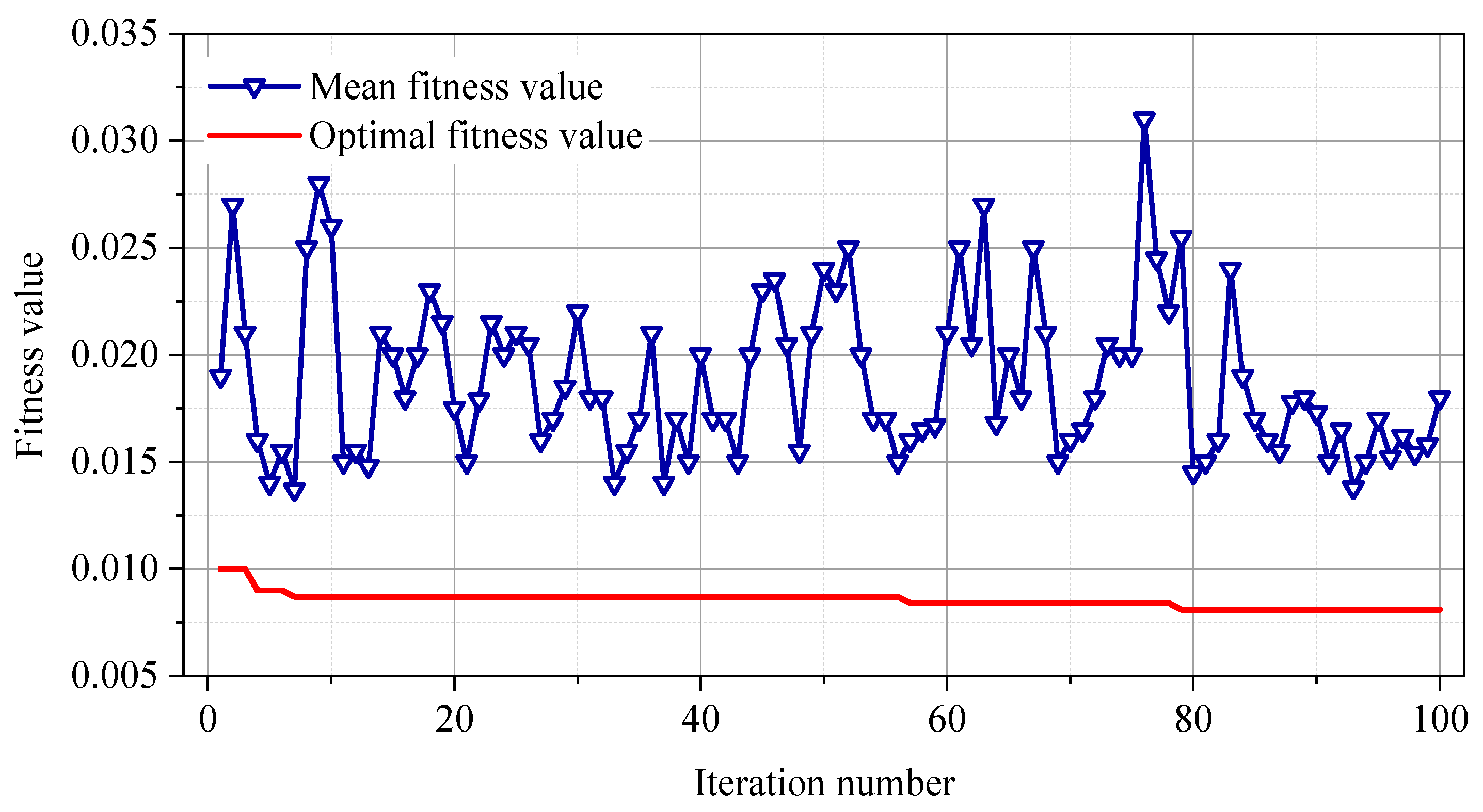
The SVM parameters are optimized by means of both PSO and five-fold cross validation. The value ranges of two parameters $C$ and $\gamma$ were set as $[0.1,100]$ and $[0.01,100]$, respectively. When using PSO for parameter optimization, the population size of the particle swarm was 20, the maximum number of iterations was 100, and two learning factors, $c_1$ and $c_2$, were separately set as 1.5 and 1.7 [48]. A group of initial particles was randomly generated in the range of parameters, and the mean square error (MSE) of cross validation [49] was selected as the fitness function. The iterative optimization process of the PSO algorithm is illustrated in Figure 2, and the fitness curve obtained can be seen in Figure 4. When the iteration number is 79, the fitness value reaches the minimum of 0.008, and the optimal parameters, $C_{best}=16.474$ and ${\gamma }_{best}=0.129$, are acquired by model training. The PSVM model with optimal parameters needs to be verified through the test set.

4.3. Performance Evaluation

On the one hand, the measured N_u values in the training set and test set were compared with the corresponding predicted values after inverse normalization. The evaluation indexes in Section 3.3 were used to quantify the PSVM model training and test results to determine whether the trained model has the problem of over-fitting or under-fitting. On the other hand, several other soft computing methods, namely decision tree (DT) [50], Gaussian process (GP) [51], and multiple linear regression (MLR) [52], were introduced for performance comparison with PSVM to demonstrate the advantages of the proposed PSVM model. Herein, MLR is the simplest regression technique, which involves finding the best fitting straight line through a set of points. DT builds regression or classification models in the form of a tree structure. GP is a nonparametric model which uses prior knowledge to conduct regression analysis of data. The three models are commonly applied in the field of structural engineering [53,54,55]. Additionally, two common design methods based on the superposition principle, GJB 4142-2000 (Chinese code) and AIJ 1997 (Japanese code) expressions, were also used for prediction comparison with PSVM.

In terms of the same training and test set, the prediction results of six methods (DT, GP, MLR, PSVM, GJB 4142-2000, and AIJ 1997 expressions) were obtained based on MATLAB^® R2016b. The performance comparisons of these calculations were visualized and quantified.

5. Results and Discussion

5.1. PSVM Training and Test Results

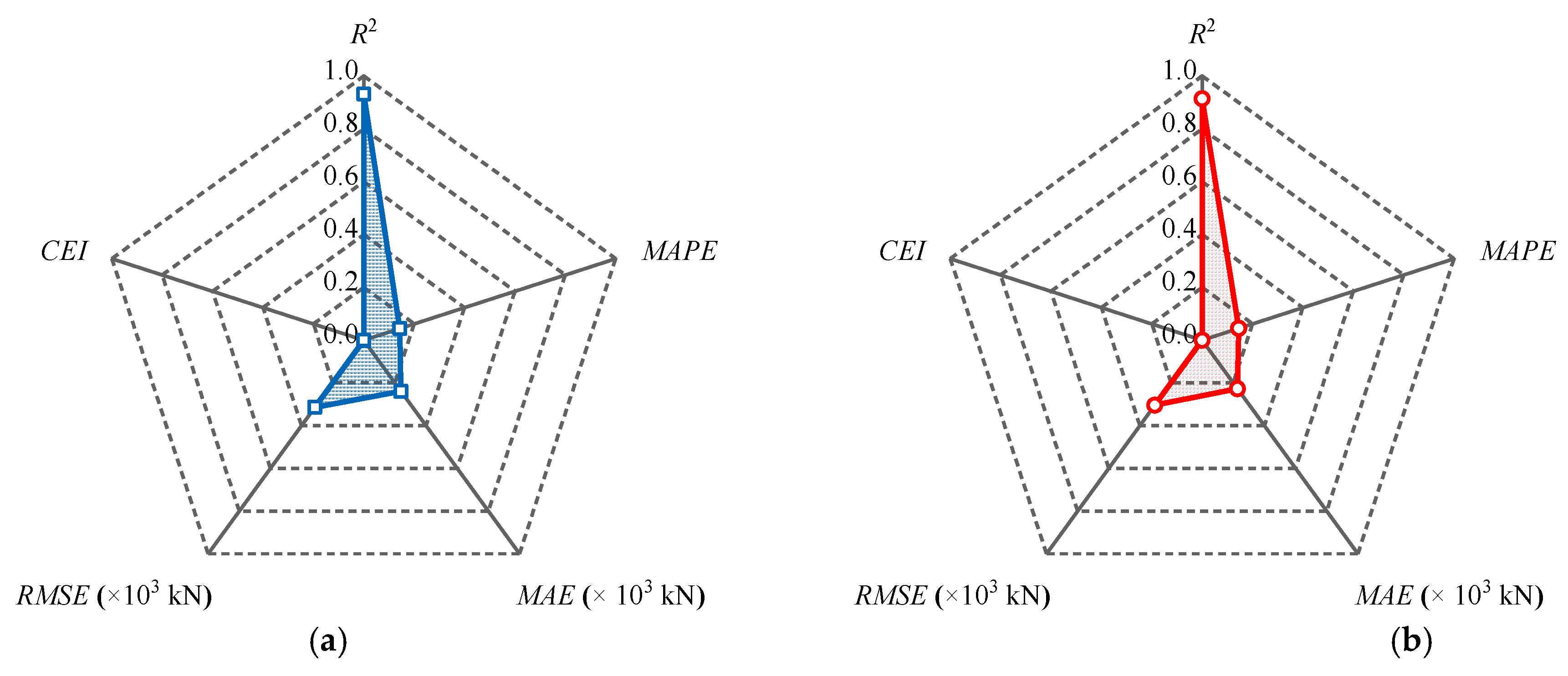
The PSVM training and test results are shown in Figure 5a,b, respectively. It can be found that the measured and estimated N_u values obtained from PSVM in the training and test sets agree with each other. The excellent prediction performance of PSVM shows that the SVM model, which adopts PSO algorithm to seek the optimal parameter combination, can capture the complex nonlinear mapping between the seven input variables and ultimate axial capacity N_u [56]. The prediction effect of PSVM is quantitatively evaluated with five statistical indexes. The performance evaluation results of PSVM training and test are seen in Figure 6a,b. Obviously, R², MAPE, MAE, and RMSE are close to 1 and CEI is 0 in both datasets, which indicates that the prediction accuracy of PSVM is relatively high. Moreover, the regions enclosed by five indexes corresponding to the PSVM training and test in the radar chart are almost coincidental, indicating that the trained PSVM model is reasonable.

5.2. Multi-Model Performance Comparison

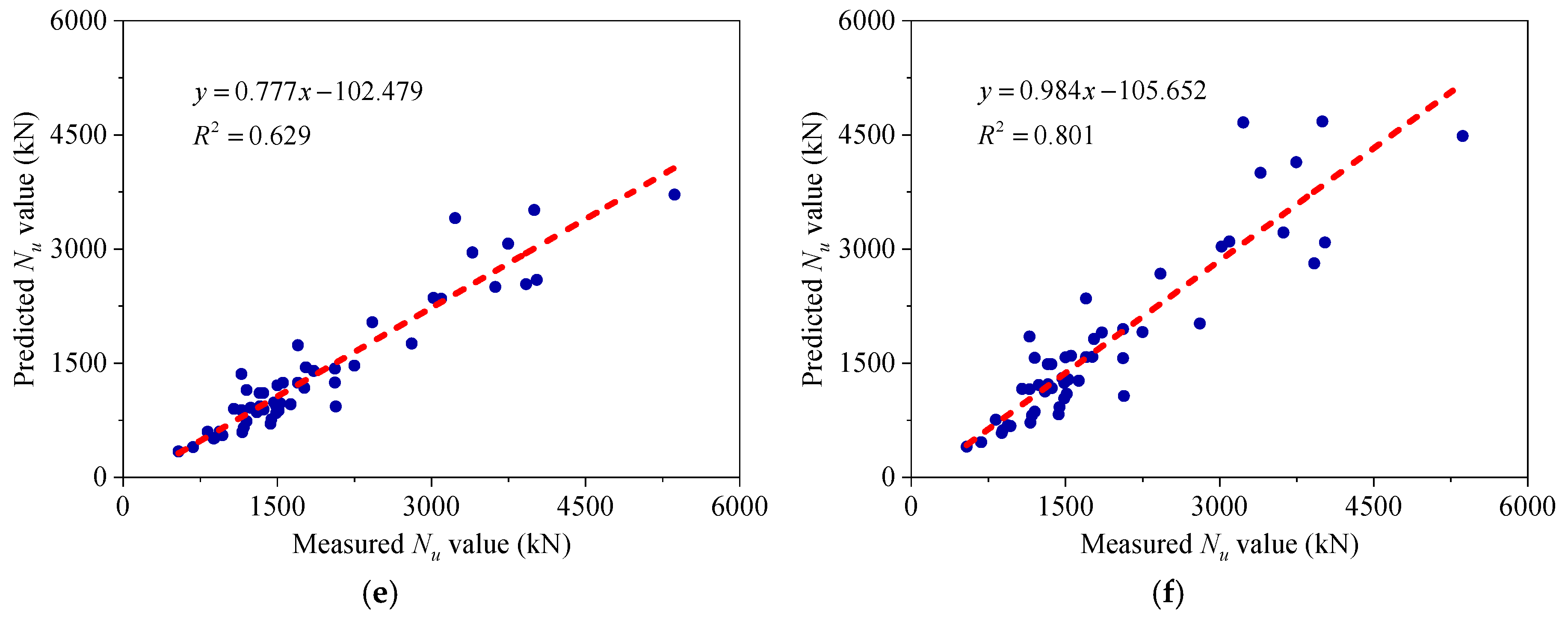
The linear fitting effects of the measured N_u values in the test set and the corresponding predicted N_u values obtained from the six different methods are shown in Figure 7. It is evident from the first four subgraphs that PSVM has the best prediction performance, followed by DT, and the worst is GP. Though MLR is a common linear model, its performance is still better than the nonlinear model of GP, indicating that the linear model is not necessarily worse than the nonlinear model. Additionally, as a combined model, the prediction performance of PSVM is better than that of a single model. This viewpoint can be proven by the performance evaluation results of different models in

Table 2. Prediction performance evaluation of DT, GP, MLR, PSVM, AIJ 1997, and GJB 4142-2000 expressions in the training set.

Evaluation Indexes	DT	GP	MLR	PSVM	AIJ 1997 Expression	GJB 4142-2000 Expression
R2	0.825	0.432	0.522	0.932	0.635	0.770
MAPE	0.204	0.512	0.320	0.143	0.316	0.210
MAE (×103 kN)	0.369	0.743	0.592	0.239	0.606	0.423
RMSE (×103 kN)	0.503	0.906	0.831	0.314	0.727	0.576
CEI	0.239	1.000	0.718	0.000	0.622	0.329

and

Table 3. Prediction performance evaluation of DT, GP, MLR, PSVM, AIJ 1997, and GJB 4142-2000 expressions in the test set.

Evaluation Indexes	DT	GP	MLR	PSVM	AIJ 1997 Expression	GJB 4142-2000 Expression
R2	0.843	0.239	0.544	0.914	0.629	0.801
MAPE	0.195	0.544	0.304	0.145	0.303	0.196
MAE (×103 kN)	0.327	0.773	0.520	0.227	0.539	0.345
RMSE (×103 kN)	0.411	0.905	0.701	0.304	0.632	0.463
CEI	0.148	1.000	0.536	0.000	0.484	0.194

. Generally speaking, the prediction accuracy of SVM optimized by PSO is about 5% higher than that of SVM optimized by the grid search technique (GST) [57]. In Section 4.2, PSO converges after less than 100 iterations, which shows that the operation efficiency of PSO is also better than that of GST. Additionally, PSO can adjust SVM parameters adaptively, so that the combined PSVM model has better generalization ability.

The last two subgraphs in Figure 7 are the calculation results of the two design methods, GJB 4142-2000 and AIJ 1997 expressions. Compared with the above four MLAs, the design expressions have physical meaning and are easy to calculate, resulting in lots of practical applications. As for prediction performance, the prediction accuracy of the two expressions is not as good as that of PSVM and DT, but better than that of MLR and GP. Combined with Table 2 and Table 3, it can be found that the calculation results of GJB are more accurate than those of AIJ, but there is still a gap with PSVM.

5.3. Prediction Error Correction

Although PSVM has a higher prediction accuracy than the other three MLAs and the two design expressions (see Section 5.2), there is still a certain error between estimated results and measured N_u values. Thus, prediction error correction becomes the key to further improve the prediction performance of PSVM. To this end, a prediction error correction method based on PSVM is proposed. (1) The output variable was changed from N_u to the relative error (abbreviated as ξ) obtained by subtracting the predicted value from the measured value, and seven input variables $(D,t,L,f_y,E_s,f_c,E_c)$ remain unchanged. According to Section 4.1, the prediction error dataset was also divided into training set (70%) and test set (30%), and the data order remained the same. (2) According to the parameter optimization process in Section 4.2, when the iteration number is 55, the fitness value reaches the minimum of 0.068, and the optimal parameters, $C_{best}=16.429$ and ${\gamma }_{best}=0.391$, are obtained. (3) The PSVM model with optimal parameters was used to make a prediction of relative error ξ. The predicted ξ values were added to the corresponding predicted N_u values in the test set (in Section 5.1) to obtain the predicted N_u results after error correction (see Figure 8). It can be found that the N_u value after error correction is closer to the measured value, especially the box selected points in Figure 8. Additionally, the evaluation indexes of corrected N_u values are better than those of original prediction results, as shown in

Table 4. Prediction performance comparison of the original PSVM model and error corrected PSVM model in the test set.

Evaluation Indexes	PSVM	PSVM after Error Correction
R2	0.914	0.953
MAPE	0.145	0.107
MAE (×103 kN)	0.227	0.176
RMSE (×103 kN)	0.304	0.226

. The improvement of prediction performance shows that the prediction error correction method is feasible and effective.

5.4. Sensitivity Analysis of Input Variables

Both Section 5.1 and 5.2 demonstrate the decent performance of the PSVM model. In order to determine the most influential input variables on the ultimate axial capacity N_u, the sensitivity analysis is performed using the cosine amplitude method (CAM) [58,59] in this section. The method has achieved good sensitivity analysis results in most research [60,61,62]. The express similarity relation between the target function and the input parameters is used to obtain by CAM [63]. In this method, each data pair $(x_i,x_j)$ can be considered as a specific point in the m-dimensional space, where each point requires m-coordinates to be fully described. Thus, each input variable is directly connected to the corresponding output. The strength of this relationship between $x_i$ and $x_j$ is calculated by:

$$r_{ij}=\frac{{\displaystyle \sum _{k=1}^m{x}_{ik}{x}_{jk}}}{\sqrt{{\displaystyle \sum _{k=1}^m{x}_{ik}^2}{\displaystyle \sum _{k=1}^m{x}_{jk}^2}}},$$

(17)

where $x_{ik}$ and $x_{jk}$ are the k-th input and corresponding k-th output variable of the model, respectively; and $m$ is the number of experimental data. The larger the $r_{ij}$ value, the greater the influence of the corresponding input variable on the output.

The sensitivity analysis results are presented in Figure 9. From a single variable, the side length $D$ of square CFST specimens has the greatest influence on the ultimate axial capacity. In terms of different variable combinations, it is obvious that the geometric properties $(D,t,L)$ of square CFST specimens have the relatively highest effects on N_u values. Therefore, the size effect (or scale effect) of square CFST short columns under axial compression is not negligible, which has long been discussed by Yamamoto et al. [64].

5.5. Discussion: Future Model Improvements

There are some deficiencies in predicting the ultimate axial capacity N_u of square CFST short columns through the proposed PSVM model, which need to be resolved in future research. (1) The amount of data used to establish the PSVM model is small, with only 180 groups of experimental data. Although the test accuracy of the trained model is over 90%, the generalizability and robustness of the model based on a small amount of data are insufficient. More high-quality experimental data needs to be collected to improve the overall performance of PSVM. (2) Some other properties that affect the ultimate axial capacity of square CFST short columns are not treated as input variables, such as steel grade, concrete age, and concrete pouring method. When many input variables are considered, feature selection is also required. (3) Four supervised learning methods (DT, GP, MLR, and SVM) and a metaheuristic optimization algorithm (PSO) were used for nonlinear regression modeling in this paper. Other advanced MLAs can be introduced to predict the ultimate axial capacity, such as multilayer perceptron [65,66] and random forest [67,68,69]. Some new optimization algorithms can also be used to improve model performance while reducing the operation time. The combined model is the development trend of the regression prediction method. (4) The proposed PSVM model is essentially a black box. In other words, the complex relationship between input and output variables is difficult to explain. The interpretability of the model needs to be studied urgently. Furthermore, feature importance analysis is also imperative before the model is applied to practical engineering, which makes it easy to adjust the geometric, steel, and concrete properties of square CFST short columns.

6. Conclusions and Perspectives

This paper mainly investigated the application of the combined PSVM model based on SVM and PSO in the prediction of ultimate axial capacity N_u of square CFST short columns. A large number of axial compression tests were utilized to obtain the experimental data needed by the prediction model. The reliability of the experimental dataset was ensured by input selection and data checking. PSO algorithm was used to optimize the parameters of SVM to achieve the optimal PSVM model. The prediction performance of the trained model was verified by an independent test set, and compared with that of the other three benchmark models and two design expressions. The prediction effect of each method was quantified by five evaluation criteria. Simulation results show that the proposed PSVM model has obvious advantages in N_u value prediction, as described below:

• The SVM optimized by PSO can accurately capture the complex nonlinear relationship between the seven input variables and the ultimate axial capacity. Thus, both model training and test results are great, and the accuracy rate is more than 90%.
• The PSO algorithm can rapidly converge after less than 100 iterations, and the MSE value corresponding to the optimal parameter combination is small, indicating that PSO is suitable for optimizing the SVM parameters.
• Compared with the other three MLAs and two expressions, the evaluation indexes of PSVM are superior. The excellent prediction performance of PSVM can reflect the enormous potential of combining mechanical property experiments with artificial intelligence algorithms.
• The proposed prediction error correction method is helpful to improve the prediction performance of PSVM. Additionally, the sensitivity analysis results are expected to simplify the design of square CFST short columns.

As such, it is believed that the proposed PSVM model can be suitably applied in engineering. Not only can the model predict the ultimate axial capacity, but can be used to estimate other mechanical properties of square CFST short columns, such as ultimate pure bending moment and fire resistance.

References

- Ji, J.; Xu, Z.; Jiang, L.; Yuan, C.; Zhang, Y.; Zhou, L.; Zhang, S. Nonlinear buckling analysis of H-type honeycombed composite column with rectangular concrete-filled steel tube flanges. Int. J. Steel Struct. 2018, 18, 1153–1166. [Google Scholar] [CrossRef]
- Han, L.H.; Li, W.; Bjorhovde, R. Developments and advanced applications of concrete-filled steel tubular (CFST) structures: Members. J. Constr. Steel Res. 2014, 100, 211–228. [Google Scholar] [CrossRef]
- Giakoumelis, G.; Lam, D. Axial capacity of circular concrete-filled tube columns. J. Constr. Steel Res. 2004, 60, 1049–1068. [Google Scholar] [CrossRef]
- Evirgen, B.; Tuncan, A.; Taskin, K. Structural behavior of concrete filled steel tubular sections (CFT/CFST) under axial compression. Thin-Walled Struct. 2014, 80, 46–56. [Google Scholar] [CrossRef]
- Li, C.X.; Campbell, B.K.; Liu, Y.M.; Yue, D.K.P. A fast multi-layer boundary element method for direct numerical simulation of sound propagation in shallow water environments. J. Comput. Phys. 2019, 392, 694–712. [Google Scholar] [CrossRef]
- Tao, Z.; Wang, Z.B.; Yu, Q. Finite element modelling of concrete-filled steel stub columns under axial compression. J. Constr. Steel Res. 2013, 89, 121–131. [Google Scholar] [CrossRef]
- Han, L.H.; An, Y.F. Performance of concrete-encased CFST stub columns under axial compression. J. Constr. Steel Res. 2014, 93, 62–76. [Google Scholar] [CrossRef]
- Lyu, X.; Xu, Y.; Xu, Q.; Yu, Y. Axial compression performance of square thin walled concrete-filled steel tube stub columns with reinforcement stiffener under constant high-temperature. Materials 2019, 12, 1098. [Google Scholar] [CrossRef]
- Liang, Q.Q. Performance-based analysis of concrete-filled steel tubular beam-columns, Part I: Theory and algorithms. J. Constr. Steel Res. 2009, 65, 363–372. [Google Scholar] [CrossRef]
- Liang, Q.Q. Performance-based analysis of concrete-filled steel tubular beam-columns, Part II: Verification and applications. J. Constr. Steel Res. 2009, 65, 351–362. [Google Scholar] [CrossRef]
- Lu, X.; Zhang, W.; Li, Y.; Ye, L. Size effect of axial strength of concrete-filled square steel tube columns. J. Shenyang Jianzhu Univ. 2012, 28, 974–980. [Google Scholar]
- Yu, X.M.; Chen, B.C. A statistical method for predicting the axial load capacity of concrete filled steel tubular columns. Int. J. Civ. Environ. Eng. 2011, 11, 20–39. [Google Scholar]
- Zheng, L.Q.; Guo, S.L.; Zhou, J.Z. Simplified model to predict load-bearing capacity of concrete-filled steel tubular laced column. Appl. Mech. Mater. 2013, 405–408, 1041–1045. [Google Scholar] [CrossRef]
- Kourou, K.; Exarchos, T.P.; Exarchos, K.P.; Karamouzis, M.V.; Fotiadis, D.I. Machine learning applications in cancer prognosis and prediction. Comput. Struct. Biotechnol. J. 2015, 13, 8–17. [Google Scholar] [CrossRef] [PubMed]
- Saadoon, A.S.; Nasser, K.Z.; Mohamed, I.Q. A neural network model to predict ultimate strength of rectangular concrete filled steel tube beam-columns. Eng. Technol. J. 2012, 30, 3328–3340. [Google Scholar]
- Saadoon, A.S.; Nasser, K.Z. Use of neural networks to predict ultimate strength of circular concrete filled steel tube beam-columns. Thi-Qar Univ. J. Eng. Sci. 2013, 4, 48–62. [Google Scholar]
- Ahmadi, M.; Naderpour, H.; Kheyroddin, A. Utilization of artificial neural networks to prediction of the capacity of CCFT short columns subject to short term axial load. Arch. Civ. Mech. Eng. 2014, 14, 510–517. [Google Scholar] [CrossRef]
- Ahmadi, M.; Naderpour, H.; Kheyroddin, A. ANN model for predicting the compressive strength of circular steel-confined concrete. Int. J. Civ. Eng. 2017, 15, 213–221. [Google Scholar] [CrossRef]
- Khalaf, A.A.; Nasser, K.Z.; Kamil, F. Predicting the ultimate strength of circular concrete filled steel tubular columns by using artificial neural networks. Int. J. Civ. Eng. Technol. 2018, 9, 1724–1736. [Google Scholar]
- Moon, J.; Kim, J.J.; Lee, T.H.; Lee, H.E. Prediction of axial load capacity of stub circular concrete-filled steel tube using fuzzy logic. J. Constr. Steel Res. 2014, 101, 184–191. [Google Scholar] [CrossRef]
- Güneyisi, E.M.; Gültekin, A.; Mermerdaş, K. Ultimate capacity prediction of axially loaded CFST short columns. Int. J. Steel Struct. 2016, 16, 99–114. [Google Scholar] [CrossRef]
- İpek, S.; Güneyisi, E.M. Ultimate axial strength of concrete-filled double skin steel tubular column sections. Adv. Civ. Eng. 2019, 6493037, 1–19. [Google Scholar] [CrossRef]
- Al-Khaleefi, A.M.; Terro, M.J.; Alex, A.P.; Wang, Y. Prediction of fire resistance of concrete filled tubular steel columns using neural networks. Fire Saf. J. 2002, 37, 339–352. [Google Scholar] [CrossRef]
- Wang, Y.; Liu, Z.Q.; Zhang, M. Prediction of mechanical behavior of concrete filled steel tube structure using artificial neural network. Appl. Mech. Mater. 2013, 368–370, 1095–1098. [Google Scholar] [CrossRef]
- Basarir, H.; Elchalakani, M.; Karrech, A. The prediction of ultimate pure bending moment of concrete-filled steel tubes by adaptive neuro-fuzzy inference system (ANFIS). Neural Comput. Appl. 2019, 31, 1239–1252. [Google Scholar] [CrossRef]
- Cortes, C.; Vapnik, V. Support-vector networks. Mach. Learn. 1995, 20, 273–297. [Google Scholar] [CrossRef]
- Yan, W.; Shao, H.; Wang, X. Soft sensing modeling based on support vector machine and Bayesian model selection. Comput. Chem. Eng. 2004, 28, 1489–1498. [Google Scholar] [CrossRef]
- Su, H.; Li, X.; Yang, B.; Wen, Z. Wavelet support vector machine-based prediction model of dam deformation. Mech. Syst. Signal Process. 2018, 110, 412–427. [Google Scholar] [CrossRef]
- Najafzadeh, M.; Etemad-Shahidi, A.; Lim, S.Y. Scour prediction in long contractions using ANFIS and SVM. Ocean Eng. 2016, 111, 128–135. [Google Scholar] [CrossRef]
- Mangalathu, S.; Jeon, J.S. Classification of failure mode and prediction of shear strength for reinforced concrete beam-column joints using machine learning techniques. Eng. Struct. 2018, 160, 85–94. [Google Scholar] [CrossRef]
- Krishnan, N.A.; Mangalathu, S.; Smedskjaer, M.M.; Tandia, A.; Burton, H.; Bauchy, M. Predicting the dissolution kinetics of silicate glasses using machine learning. J. Non-Crystal. Sol. 2018, 487, 37–45. [Google Scholar] [CrossRef] [Green Version]
- Li, Q.; Meng, Q.; Cai, J.; Yoshino, H.; Mochida, A. Predicting hourly cooling load in the building: A comparison of support vector machine and different artificial neural networks. Energy Convers. Manag. 2009, 50, 90–96. [Google Scholar] [CrossRef]
- Poli, R.; Kennedy, J.; Blackwell, T. Particle swarm optimization. Swarm Intell. 2007, 1, 33–57. [Google Scholar] [CrossRef]
- Goldberg, D.E.; Holland, J.H. Genetic algorithms and machine learning. Mach. Learn. 1988, 3, 95–99. [Google Scholar] [CrossRef]
- Wang, Y.; Chen, P.; Liu, C.; Zhang, Y. Size effect of circular concrete-filled steel tubular short columns subjected to axial compression. Thin-Walled Struct. 2017, 120, 397–407. [Google Scholar] [CrossRef]
- Tian, Y. Experimental Research on Size Effect of Concrete-Filled Steel Tubular Stub Columns under Axial Compressive Load. Master’s Thesis, Harbin Institute of Technology, Harbin, China, July 2014. [Google Scholar]
- Yao, G.H.; Han, L.H. primary research on calculations for bearing capacity of concrete filled high strength steel tubular members. Ind. Constr. 2007, 2, 96–99. [Google Scholar]
- Heddam, S.; Kisi, O. Modelling daily dissolved oxygen concentration using least square support vector machine, multivariate adaptive regression splines and M5 model tree. J. Hydrol. 2018, 559, 499–509. [Google Scholar] [CrossRef]
- Suykens, J.A.; Vandewalle, J. Least squares support vector machine classifiers. Neural Process. Lett. 1999, 9, 293–300. [Google Scholar] [CrossRef]
- Pedregosa, F.; Varoquaux, G.; Gramfort, A.; Michel, V.; Thirion, B.; Grisel, O.; Blondel, M.; Prettenhofer, P.; Weiss, R.; Dubourg, V.; et al. Scikit-learn: Machine learning in Python. J. Mach. Learn. Res. 2011, 12, 2825–2830. [Google Scholar]
- Kennedy, J.; Eberhart, R. Particle swarm optimization. In Proceedings of the IEEE International Conference on Neural Networks, Perth, Australia, 27 November–1 December 1995; Volume 4, pp. 1942–1948. [Google Scholar]
- Yan, J.; Xu, Z.; Yu, Y.; Xu, H.; Gao, K. Application of a hybrid optimized BP network model to estimate water quality parameters of Beihai Lake in Beijing. Appl. Sci. 2019, 9, 1863. [Google Scholar] [CrossRef]
- Ly, H.B.; Le, L.M.; Duong, H.T.; Nguyen, T.C.; Pham, T.A.; Le, T.T.; Le, V.M.; Nguyen-Ngoc, L.; Pham, B.T. Hybrid artificial intelligence approaches for predicting critical buckling load of structural members under compression considering the influence of initial geometric imperfections. Appl. Sci. 2019, 9, 2258. [Google Scholar] [CrossRef]
- Dao, D.V.; Trinh, S.H.; Ly, H.B.; Pham, B.T. Prediction of compressive strength of geopolymer concrete using entirely steel slag aggregates: Novel hybrid artificial intelligence approaches. Appl. Sci. 2019, 9, 1113. [Google Scholar] [CrossRef]
- Chen, H.; Asteris, P.G.; Jahed Armaghani, D.; Gordan, B.; Pham, B.T. Assessing dynamic conditions of the retaining wall: Developing two hybrid intelligent models. Appl. Sci. 2019, 9, 1042. [Google Scholar] [CrossRef]
- Moradi, M.J.; Hariri-Ardebili, M.A. Developing a library of shear walls database and the neural network based predictive meta-model. Appl. Sci. 2019, 9, 2562. [Google Scholar] [CrossRef]
- Kotsiantis, S.B.; Kanellopoulos, D.; Pintelas, P.E. Data preprocessing for supervised leaning. Int. J. Comput. Sci. 2006, 1, 111–117. [Google Scholar]
- Ranaee, V.; Ebrahimzadeh, A.; Ghaderi, R. Application of the PSO-SVM model for recognition of control chart patterns. ISA Trans. 2010, 49, 577–586. [Google Scholar] [CrossRef]
- Toghyani, S.; Ahmadi, M.H.; Kasaeian, A.; Mohammadi, A.H. Artificial neural network, ANN-PSO and ANN-ICA for modelling the Stirling engine. Int. J. Ambient Energy 2016, 37, 456–468. [Google Scholar] [CrossRef]
- Tso, G.K.; Yau, K.K. Predicting electricity energy consumption: A comparison of regression analysis, decision tree and neural networks. Energy 2007, 32, 1761–1768. [Google Scholar] [CrossRef]
- Zhang, M.; Li, M.; Shen, Y.; Ren, Q.; Zhang, J. Multiple mechanical properties prediction of hydraulic concrete in the form of combined damming by experimental data mining. Constr. Build. Mater. 2019, 207, 661–671. [Google Scholar] [CrossRef]
- Sousa, S.I.V.; Martins, F.G.; Alvim-Ferraz, M.C.M.; Pereira, M.C. Multiple linear regression and artificial neural networks based on principal components to predict ozone concentrations. Environ. Model. Softw. 2007, 22, 97–103. [Google Scholar] [CrossRef]
- Salazar, F.; Toledo, M.Á.; Oñate, E.; Suárez, B. Interpretation of dam deformation and leakage with boosted regression trees. Eng. Struct. 2016, 119, 230–251. [Google Scholar] [CrossRef] [Green Version]
- Corrado, N.; Durrande, N.; Gherlone, M.; Hensman, J.; Mattone, M.; Surace, C. Single and multiple crack localization in beam-like structures using a Gaussian process regression approach. J. Vib. Control 2018, 24, 4160–4175. [Google Scholar] [CrossRef]
- Janani, S.; Santhi, A.S. Multiple linear regression model for mechanical properties and impact resistance of concrete with fly ash and hooked-end steel fibers. Int. J. Technol. 2018, 9, 526–536. [Google Scholar] [CrossRef]
- Lu, X.; Zou, W.; Huang, M. A novel spatiotemporal LS-SVM method for complex distributed parameter systems with applications to curing thermal process. IEEE Trans. Ind. Inf. 2016, 12, 1156–1165. [Google Scholar] [CrossRef]
- Lin, S.W.; Ying, K.C.; Chen, S.C.; Lee, Z.J. Particle swarm optimization for parameter determination and feature selection of support vector machines. Expert Syst. Appl. 2008, 35, 1817–1824. [Google Scholar] [CrossRef]
- Yang, Y.; Zhang, Q. A hierarchical analysis for rock engineering using artificial neural networks. Rock Mech. Rock Eng. 1997, 30, 207–222. [Google Scholar] [CrossRef]
- Sayadi, A.; Monjezi, M.; Talebi, N.; Khandelwal, M. A comparative study on the application of various artificial neural networks to simultaneous prediction of rock fragmentation and backbreak. J. Rock Mech. Geotech. Eng. 2013, 5, 318–324. [Google Scholar] [CrossRef] [Green Version]
- Rezaei, M. Indirect measurement of the elastic modulus of intact rocks using the Mamdani fuzzy inference system. Measurement 2018, 129, 319–331. [Google Scholar] [CrossRef]
- Mottahedi, A.; Sereshki, F.; Ataei, M. Overbreak prediction in underground excavations using hybrid ANFIS-PSO model. Tunn. Undergr. Space Technol. 2018, 80, 1–9. [Google Scholar] [CrossRef]
- Hasanipanah, M.; Amnieh, H.B.; Arab, H.; Zamzam, M.S. Feasibility of PSO-ANFIS model to estimate rock fragmentation produced by mine blasting. Neural Comput. Appl. 2018, 30, 1015–1024. [Google Scholar] [CrossRef]
- Ghorbani, A.; Hasanzadehshooiili, H.; Ghamari, E.; Medzvieckas, J. Comprehensive three dimensional finite element analysis, parametric study and sensitivity analysis on the seismic performance of soil–micropile-superstructure interaction. Soil Dyn. Earthq. Eng. 2014, 58, 21–36. [Google Scholar] [CrossRef]
- Yamamoto, T.; Kawaguchi, J.; Morino, S. Experimental study of scale effects on the compressive behavior of short concrete-filled steel tube columns. Compos. Constr. Steel Concr. 2000, 25, 27–44. [Google Scholar] [CrossRef]
- Ghorbani, M.A.; Deo, R.C.; Yaseen, Z.M.; Kashani, M.H.; Mohammadi, B. Pan evaporation prediction using a hybrid multilayer perceptron-firefly algorithm (MLP-FFA) model: Case study in North Iran. Theor. Appl. Climatol. 2018, 133, 1119–1131. [Google Scholar] [CrossRef]
- Demirpolat, A.B.; Das, M. Prediction of viscosity values of nanofluids at different pH values by alternating decision tree and multilayer perceptron methods. Appl. Sci. 2019, 9, 1288. [Google Scholar] [CrossRef]
- Dai, B.; Gu, C.; Zhao, E.; Qin, X. Statistical model optimized random forest regression model for concrete dam deformation monitoring. Struct. Control Health Monit. 2018, 25, e2170. [Google Scholar] [CrossRef]
- Ren, Q.; Wang, G.; Li, M.; Han, S. Prediction of rock compressive strength using machine learning algorithms based on spectrum analysis of geological hammer. Geotech. Geol. Eng. 2019, 37, 475–489. [Google Scholar] [CrossRef]
- Zhou, J.; Li, E.; Wei, H.; Li, C.; Qiao, Q.; Armaghani, D.J. Random forests and Cubist algorithms for predicting shear strengths of rockfill materials. Appl. Sci. 2019, 9, 1621. [Google Scholar] [CrossRef]
Figure 1.
Schematic diagram of the axial compression test device for square concrete-filled steel tubular (CFST) short columns: (a) front view; (b) section view of the specimen.
Figure 2.
Architecture description of the proposed PSVM model.
Figure 3.
Correlation matrix of seven input variables.
Figure 4.
Particle swarm optimization (PSO) iterative optimization curve.
Figure 5.
Measured and estimated Nu values obtained from PSVM in the (a) training set and (b) test set.
Figure 6.
Radar chart of performance evaluation of PSVM in the (a) training set and (b) test set.
Figure 7.
Coefficient of determination (R2) of the measured and predicted Nu values in the test set using (a) decision tree (DT); (b) Gaussian process (GP); (c) multiple linear regression (MLR); (d) PSVM; (e) AIJ 1997 expression; (f) GJB 4142-2000 expression.
Figure 8.
Measured and estimated Nu values obtained from the original PSVM model and error corrected PSVM model in the test set.
Figure 9.
Sensitivity analysis results of seven input variables on the output Nu.