A Sparse Model of Guided Wave Tomography for Corrosion Mapping in Structure Health Monitoring Applications

1
The Department of Electrical Engineering, Shanghai Dianji University, Shanghai 201306, China
2
Research Center of Smart Networks and Systems, The Department of Electronic Engineering, Fudan University, Shanghai 200433, China
*
Author to whom correspondence should be addressed.
Appl. Sci. 2019, 9(15), 3126; https://doi.org/10.3390/app9153126
Submission received: 1 March 2019
/
Revised: 5 July 2019
/
Accepted: 26 July 2019
/
Published: 1 August 2019
(This article belongs to the Special Issue Structural Damage Detection and Health Monitoring)
Abstract
:To improve the reconstruction image spatial resolutions of ultrasonic guided wave ray tomography, a sparse model, based on the differences between the inspected and original slowness of the ultrasonic guided waves propagating in the plate-like or pipe-like materials, is first proposed in this paper. Unlike the conventional ultrasonic guided wave tomography whose reconstruction image resolutions are limited by an underdetermined linear model, analyses show that our new model, although it is also underdetermined, can give the optimal solution of the reconstruction image when the constraints on the sparsity of the slowness difference distribution are valid. The reason for the validation of the sparse constraints on the corrosions of the materials is explained. Based on our new model, a least absolute shrinkage and selection operator (LASSO) approach to do the thickness change mapping of a structure health monitoring (SHM) application is then formulated. Analyses also show that the visible artifacts can be avoided using our method, and the spatial resolutions of reconstruction image by our approach can further be improved by increasing the number of grids in the calculation. The approach is validated by experimental work on an aluminum plate. It is also shown that compared to the conventional ray tomography, the presented method can achieve a relatively high spatial resolution, with good suppression of artifacts.
1. Introduction
It is well-known that corrosion detection and monitoring are vital for preserving material integrity and extending the life cycle of, for example, industrial infrastructure, aircrafts, pipelines, and oil installations [1,2,3,4]. In many structure health monitoring (SHM) applications, ultrasonic guided wave tomography is used as a reliable tool for detecting and monitoring corrosion [5,6,7,8,9,10,11]. Sizing the corrosion region in a plate-like or a pipe-like structure is very important for corrosion detection and monitoring [12,13,14]. Conventional ultrasonic corrosion mapping is carried out by point-by-point scanning on the surface of the materials [15,16] and calculating the thickness from the arrival time of the reflected waves. In contrast, in guided wave tomography, the guided wave is excited in a plate or a pipe, passing through the monitoring area, and measured by a surrounding transducer array. The corrosion area can then be obtained by reconstructing a velocity map of the guided wave and converting it to a thickness map.
Ray tomography uses the guided wave time-of-flight (TOF) to reconstruct the slowness distribution [17,18]. However, the reconstruction via this method is of a relatively low resolution, which is limited by the width of the first Fresnel zone. In Reference [19], a wave speed map is reconstructed using the curved ray tomography with simulation, even though the size of a sound speed anomaly is smaller than the resolution length of the inversion method. Diffraction tomography implements a higher resolution using the Born approximation if the scattering generated by the corrosion is very weak [20,21]. It is clear that it is unlikely to be such a case for many corrosions of interest. The hybrid algorithm reported in Reference [22] initially uses a low-resolution ray tomography, and later gradually iterates with a diffraction tomography which can achieve a high-resolution tomography, when the scattering is not very weak. However, its performance relies on the background estimate being sufficiently accurate via ray tomography. Besides on these three tomography algorithms, the full wave-form inversion (FWI) method presents a novel nonlinear inverse scattering model to implement reconstruction images of guided wave tomography [23]. Compared with diffraction tomography, FWI allows higher order diffraction and scattering and has the same theoretical resolution limit [24]. Literature [14,25,26] also report that more accurate inversion results are achieved when this method is applied to monitor the plate-like materials. The major limitation of this method is its computational complexity and cost, and it can be acceptable as an offline imaging method. Because of the low computational complexity of ray tomography, it is widely used in many online SHM applications, such as the chemical industry and aviation industry [27]. Ray tomography is a promising method for corrosion monitoring, especially for online applications.
In this paper, the method based on ray tomography for corrosion monitoring is studied. Currently, the simultaneous iterative reconstruction technique (SIRT) [28] is a widespread used method in the ray tomography. This method is based on an underdetermined linear model. Such a linear model known is an infinite number of solutions, which can fit measured data. It means that the solution obtained by the conventional iterative reconstruction technique cannot be guaranteed as the optimal one. In order to cope with this problem, a sparse model based on differences between the inspected and original slowness of guided waves as an imaging approach for mapping plate thickness by using ray tomography is proposed in this paper. Although our model is also underdetermined, the optimal solution of the reconstruction image can be given when the constraints on the sparsity of the slowness difference distribution are valid. Based on our model, the LASSO approach is applied to obtain the solution of the sparse-constrained minimization problem. The corrosion mapping can thus be achieved. As the number of grids increase, the spatial resolutions of reconstruction image can further be improved. To verify the effectiveness of our model and approach, the experiments are conducted. Experimental results will show that we can achieve a higher resolution than SIRT, while the visible artifacts of the reconstruction images are avoided.
The remainders of this paper are organized as follows. In Section 2, both the conventional and our models for thickness change mapping via ultrasonic guided wave ray tomography is introduced and given. Then, the reconstruction method using convex sparse regularization is reported. The reason why the proposed model and method can improve the tomographic reconstruction resolution is illustrated. In Section 3, the experimental setup for the health monitoring of an aluminum plate is conducted. The experimental results used to demonstrate the correctness of the proposed model and method are reported in Section 4. The discussion is followed in Section 5. Finally, conclusions are drawn in Section 6.
2. Model for Ultrasonic Guided Wave Ray Tomography
2.1. Conventional Model
Suppose that the ultrasound transducers are arranged into two uniform linear arrays as shown in Figure 1. The left array is the transmitting one, while the right array is the receiving one. The two arrays are respectively with M ultrasound transmitters and receivers, where M is a user parameter. The arrays can be mounted on a plate-like material. Figure 1 is an example, in which each array with eight ultrasound transducers is mounted on a plate. The system operation is that the ultrasound transducers in the transmitting array are used one by one to transmit a guided wave, while all of the receivers are exploited to receive the excited guided wave. For example, when a transmitter in a given time, transmitter 1 in Figure 1, is used to excite a guided wave, all of the ultrasound transducers in the receiving array 1 to 8 are exploited to receive the excited guided wave at the same time. Once all of the receiving data have been recorded, transmitter 2 is then used to excite another guided wave. Similarly, all of the receiving transducers 1 to 8 also record the excited guided wave. This process is repeated until each transducer in the transmitting array sends the guided waves at least once. Next, all of the recorded data from the receiving array are used by a computer to perform thickness mapping.
Before the thickness mapping, the guided wave TOF should first be estimated from the recorded data. In order to improve the accuracy of the arrival time extraction, based on the known dispersion curve and the propagation distance between each pair of source and receive transducers [29,30], the dispersion compensation for the incident and transmitted A0 guided mode is implemented by the Equations (3,4) in Reference [31] without taking the mode conversion into consideration. Then the signal envelope is obtained using the Hilbert Transform. TOF is determined by the maxima of the wave envelope [32].
When a plate-like material is corroded, it is known that its thickness is changed. From the dispersion curve of the guided wave, it has been understood that the thickness changes of the material will result in the group velocity changes of the guided wave propagated in it. This finding means that the guided wave TOF will also vary accordingly. Once the group velocity of the guided wave is derived from the TOF, the thickness of the plate-like material can be obtained from the relationship between the group velocity of the guided wave propagated on the plate-like material and its thickness. The following two assumptions are set to obtain such a relationship. The first assumption is that the guide wave travels in a straight line, regardless of whether the corrosion exists on the line. The second assumption is that the corrosion is large relative to the wavelength of the guided wave. Thus, the effects of diffraction can be neglected. Based on the above assumptions, the eikonal equations given in Reference [33], when expressed by the guided wave, can be written as follows:
where is the group velocity of the guided wave, and is the TOF of the wavepacket. The represents the absolute value. By integrating both sides of Equation (1), one has
where is the location of the guided wave on a propagation path, is the group velocity of the guided wave at position , and is the infinitesimal length along the propagation path. Clearly, Equation (2) is nonlinear. For the convenience of the calculation, the monitored area is divided into grids , as shown in Figure 1. In this way, each propagation path between the transmitter and receiver is divided into small pieces by these grids. Suppose that the group velocity in each grid is constant, Equation (2) can be discretized as:
where is the length of the ith propagation path in the jth grid, as shown in Figure 1, represents the slowness in the jth grid. For grids and propagation paths, Equation (3) can be rewritten as the following linear equation:
where is the column vector of travel-time, is the column vector of slowness, and is the length matrix of the propagation paths divided into pieces by the grids. Equation (4) is known as the conventional model for ultrasonic guided wave ray tomography. By solving Equation (4), one can obtain the slowness of each grid. Based on the slowness obtained, the thickness mapping is performed. Additionally, it is obvious that the more the number of grids is, the higher the spatial resolution is. For high spatial resolution, N2 is much larger than M2. Unfortunately, when N2 > M2, Equation (4) is underdetermined. This means that the vector cannot uniquely be determined by solving Equation (4). Even so, an iterative technique called the SIRT is constantly used to do so because another alternative is unavailable so far. The SIRT is started with an initial guess of the solution and then iteratively updates the solution until some criteria are met. It is known that the solution obtained by the SIRT can only be regarded as one of all possible solutions of the underdetermined equation. This is the main reason believed why the thickness mapping reconstructed by the SIRT contains so many artifacts.
2.2. A Sparse Model
Suppose that there is no corrosion on the monitored plate-like material before its structure is investigated. Let the system shown in Figure 1 work on the plate-like material. In this way, one can obtain the measurements denoted as . Obviously, these measurements will not include any corrosion on the inspected material. Certainly, one can also obtain these measurements via a reference plate, which is exactly the same as the monitored plate-like material but without any corrosion on it. By inserting into Equation (4), one has
where assumed is the original slowness. After is obtained, let the system begin its monitor work. It means that the baseline signal and the monitored signal are measured from the same structure. Meanwhile, one may continuously or intermittently obtain the measurements T described by Equation (4). If Equation (5) is subtracted by Equation (4), one gets
Let and denote the differences of the slowness and TOF respectively. One can rewrite Equation (6) as
Assuming that the slowness does not change when the corrosion does not occur, and there is not a change of environmental or operational conditions between the baseline and the inspection. It means that the slowness difference between the inspected slowness and original slowness of every grid would be 0. It is understood that corrosion of the plate-like materials is a slow process. Corrosion slowly grows larger. When a small partial monitored plate is corroded, the slowness difference of small partial grids is changed. Figure 2 shows an example. The monitored area is divided into grids. Assuming that two grids are corroded, and the slowness in these two grids is changed.
It is obvious that most elements of are 0.
From Equation (7), the number of equations is M2, and the number of elements in , namely, the number of solutions, is N2. Since M2 is smaller than N2, Equation (7) is an underdetermined equation. However, most elements in are 0. Assuming that K is the number of non-zero values in , if K is much smaller than N2, Equation (7) can be viewed as a sparse model. The simple sparsity constraint on the slowness difference is the l0-norm constraint, i.e., , which means that the non-zero elements in is much smaller than the number of elements in . However, the solution of Equation (7) cannot be achieved with the l0-norm constraint because it is a well-known NP-hard problem. In order to cope with the NP-hard problem, the l1-norm constraint including the l0-norm constrain as its subset is used. Meanwhile, although Equation (7) is also underdetermined, its optimal solution may be obtained because of the sparsity of .
2.3. Solution of the Sparse Model
It has been understood that, when the excited frequency of a guide wave transmitted on a plate is fixed, the group velocity or slowness of the guided wave known from the dispersion curve is mainly dependent on the thickness of the plate. Namely, the slowness of the plate varies with its thickness. When a plate is corroded, the plate thickness will be changed. Suppose that the thickness of a monitored plate is fixed. It means that the upper limit of the variable thickness of the plate will be its maximum thickness. According to the maximum variable thickness of the plate, the maximum variable slowness is . Therefore, the maximum value of the difference slowness for each grid in Equation (7) can be limited as:
When the monitored area is divided into grids, one has
or, equivalently,
The denotes the lp-norm of a vector. When p = 2, the lp-norm is the Euclidean one. When is fixed, will be a constant. In such a situation, it is known that the solution of Equation (7) can be formulated as the following optimization problem
Equation (11) can equivalently be rewritten as the following least absolute shrinkage and selection operator (LASSO) problem [34]:
where is a regularization parameter. Equation (12) imposes an l1-norm on the . Owing to the nature of the l1-norm, it is well known that the LASSO problem can continuously be shrunk and do automatic variable selection to find the solutions. Many of the solutions, (i = 1,2, …, N2), are set to 0. It means that the solutions of Equation (12) are of a natural sparsity structure. Therefore, the sparsity of is naturally used in the solving process. In addition, it is well known that the LASSO problem is a convex optimization problem [34]. A convex optimization problem has an optimal solution. Thus, the optimal solutions of the reconstruction image can be obtained by the LASSO approach.
Certainly, based on our sparse model, both the SIRT and the regularization methods can be used to do defect imaging. Compared to the other regulation methods, the LASSO method has two main advantages as given in Reference [35]. First, it can achieve good estimation and prediction by shrinking the estimator towards 0. It means that the sparse solution of the sparse model can be obtained by the LASSO method but the other regularization methods for the lp-norm with p > 1 cannot. For p < 1, their solutions are sparse but the problem is not convex and this makes the minimization very challenging computationally [36]. When the solution is not sparse, it means that many of the solutions, (i = 1,2, …, N2), are not 0. It also implies that the visible artifacts are generated. Second, there is a simple iteration way available for LASSO to converge fast, which make it very attractive computationally in terms of central processing unit and memory.
Before solving Equation (12), should be known a priori. The empirical range of is from 0.0001 to 0.01. for every , can be obtained by using the CVX toolbox [37,38] to solve Equation (12). The curve with a log–log plot of versus as is varied, is then acquired. The curve is called the L-curve. After that, the optimal is calculated from the L-curve by Equation (11) of Reference [39]. In our experiments, the optimal calculated by this method is 0.001.
The flow of our method is shown in Figure 3. The received signals in the plate-like material without defects are recorded and their TOFs are extracted as the original TOFs. Then, the plate-like material is defected and the received signals in this plate-like material with defects are recorded and their TOFs are extracted as the inspected TOFs. Our sparse model is used, and the defects can be imaged by Equation (12).
3. Experimental Setup
Our experimental system consisted of a computer, an arbitrary waveform generator, a power amplifier, an oscilloscope and ultrasound transducers. Its schematic diagram is shown in Figure 4a. Piezoelectric transducers (PZTs) were employed as the ultrasound transducers in our SHM system, where the diameter of each PZT was 5 mm. The central frequency of the transducer was 250 KHz. There were 20 transducers in the transmitting and receiving arrays respectively, which were attached to a monitored aluminum plate with the dimension of 500 mm × 500 mm × 1.5 mm. The transducer spacing was 10 mm for both the transmitting and receiving arrays. The distance between the two arrays was 200 mm. Therefore, the monitored area was 200 × 200 mm2. The monitored area was divided into different numbers of grids.
A five-cycle Hanning-windowed sinusoidal signal with a central frequency of 250 KHz, which was generated using an arbitrary waveform generator (33220 A, manufactured by Agilent Technologies, Santa Clara, CA, USA) and then amplified using a power amplifier (AG1021, manufactured by T and C Power Conversion, Inc., Rochester, NY, USA), was sent to the transmitters. An oscilloscope (54622A, manufactured by Agilent Technologies, Santa Clara, CA, USA) was employed to sample the ultrasonic signals received by the receivers. A computer was used to read the sample data from the oscilloscope. Figure 4b shows a typical original received signal, where both the transmitter and receiver transducer were 10rd ones. The received signal contained A0 and S0 guided modes. From Figure 4b, it can be seen that the amplitude of the A0 guided mode was greater than that of S0. To ensure the imaging quality, a time gating function similar to Reference [40] was applied to remove unwanted components. The gating function was set to one between the start time and the end time. Outside the region, the gating function reduced from one to zero. The received signal was enveloped via a Hilbert transform. The arrival time of the S0 guided mode was taken as the maxima of the S0 guided mode envelope. The start time was taken as the arrival time of the S0 guided mode plus 200 µs. The end time was taken as the start time plus 500 µs. After that, the A0 guided mode was reserved to extract the TOF. The A0 guided mode was enveloped via a Hilbert transform. The TOF was taken as the point at which the enveloped signal intersected a threshold at 50% of the signal’s maximum. The TOF was then employed for the inversion.
4. Experimental Results
4.1. Single Regular Defect
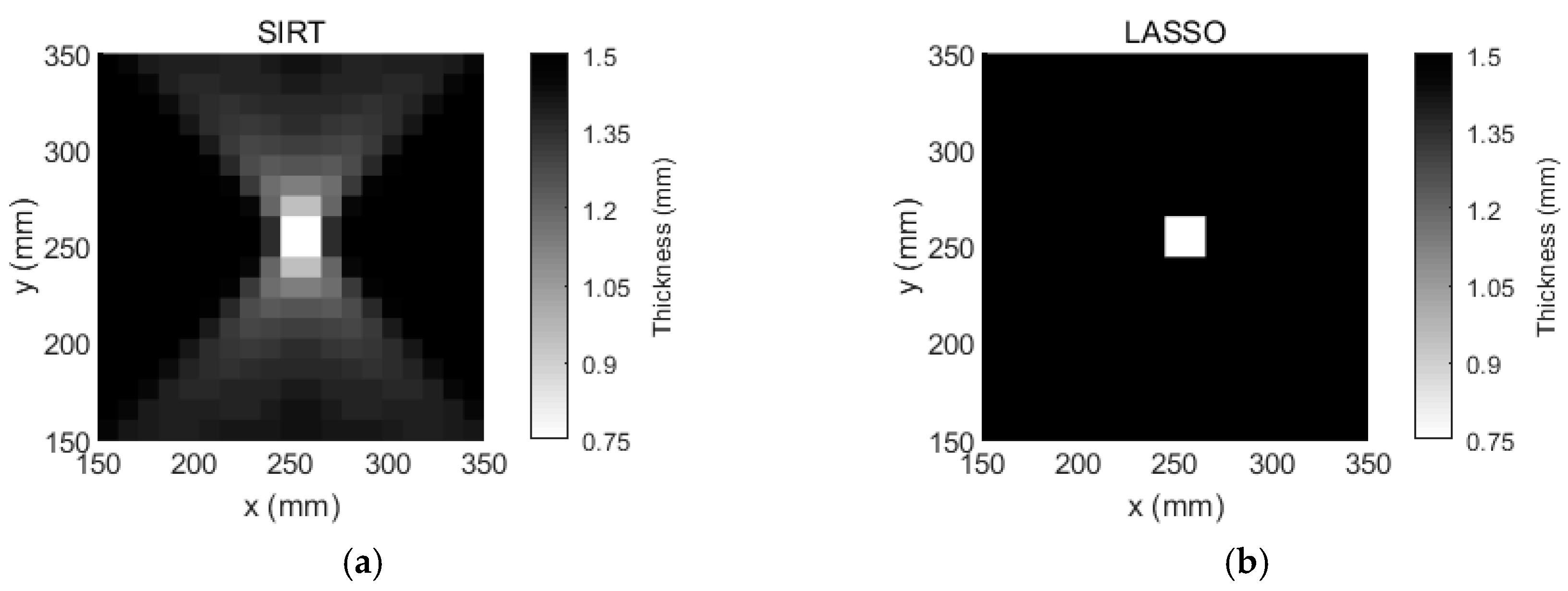
The monitored aluminum plate with a 20 mm diameter circular flat-bottomed hole in the center was made so that its thickness loss was 50%, as shown in Figure 5a. The transmitter transducers were excited one by one, and the receiver transducers recorded all the received signals. Take the 10th transmitter and receiver transducers as an example. The baseline guided wave signal and the guided wave signal passing through the defect are illustrated in Figure 5b. The monitored area was divided into 80 × 80 grids. The tomographic images reconstructed using the SIRT and our Equation (12) are shown in Figure 5c,d. From Figure 5c, it can be seen that the spatial resolution of the tomographic reconstruction with the SIRT was relatively low, and the distinct artifacts can be found. On the contrary, from Figure 5d, it can be found that the spatial resolution of the tomographic reconstruction with our Equation (12) was relatively high, and the visible artifacts in the image did not exist.
Next, the monitored area was divided into 20 × 20, 40 × 40, 60 × 60 and 80 × 80 grids respectively. The tomographic images reconstructed using the SIRT are shown in Figure 6a–d. It can be seen that the tomographic images reconstructed using the SIRT had a relatively low spatial resolution. Even if the grid density was increased, both the reconstruction spatial resolutions and the edges of the corrosion area still kept fuzziness. By contrast, Figure 7a–d are the reconstruction images using our method. These tomographic images show that they have relatively high spatial resolutions. With the increasing of the grid density, the edges of corrosion area were gradually distinct. The number of grids with the thickness changing imaged by the SIRT and our method was statistically analyzed, and the statistics result is shown in Table 1. It can be seen that the number of grids calculated by our methods with different grid density was almost the same as the area covered by the actual corrosion ones.
4.2. Two Regular Defects
The second experiment in which there were two 20 mm diameter circular flat-bottomed holes in the monitored aluminum was conducted, as shown in Figure 8a. One of the holes, whose thickness loss was 50%, was in the center of the plate. The center coordinate of another hole was x = 220 mm, y = 290 mm, whose thickness loss was 30%. The monitored area was divided into 80 × 80 grids. The tomographic images reconstructed using the SIRT and our Equation (12) are shown in Figure 8b,c. From Figure 8b, it can be seen that the tomographic reconstruction results using the SIRT confused the defect of the lower thickness loss with the artifacts. By contrast, Figure 8c obtained using the method in this paper clearly shows both the thickness losses on the plate.
The monitored area was also respectively divided into 20 × 20, 40 × 40, 60 × 60 and 80 × 80 grids. The tomographic images reconstructed using the SIRT are shown in Figure 9a–d. From Figure 9a–d, it is clear that using the SIRT, two corrosion areas cannot be easily distinguished. Even if the grid density was increased, the corrosion area of the low thickness loss was confused with the artifacts. By contrast, Figure 10a–d are the tomographic reconstruction images using our method. These tomographic images show that our method could easily identify two corrosion areas, and with an increasing grid density, the detail of corrosion area was gradually clearer. It can also be seen that the number of grids calculated by our methods with different grid density was almost the same as the areas covered by the actual corrosion ones, as shown in Table 2.
4.3. Two Partiall
The third experiment in which there were two eccentric circular flat-bottomed holes in the monitored aluminum, as shown in Figure 11a, was conducted. One of the holes, whose thickness loss was 30% and diameter was 30 mm, was in the center of the plate. The center coordinate of another hole was x = 260 mm, y = 260 mm, whose thickness loss was 50% and diameter was 40 mm. The monitored area was divided into 60 × 60 grids. The tomographic images reconstructed using the SIRT and our Equation (12) are shown in Figure 11b,c. From Figure 11b, it can be seen that the tomographic reconstruction results using the SIRT could not distinguish the defect of different thickness loss. By contrast, Figure 10c obtained using the method in this paper clearly shows all the thickness losses on the plate.
The cross sections of Figure 11a with the corrosion depths are shown in Figure 12a,b. It can be seen that the depth estimation results of our method were better than SIRT in most cases, especially along the vertical line marked in Figure 11a. However, the depth estimation results of the thinnest thickness were worse than SIRT.
5. Discussion
The results presented in this paper have shown that our approach obtained higher spatial resolution thickness mapping for plate-like structures using a sparse model than that of SIRT, and the visible artifacts in the tomographic reconstruction images were avoided. The computation time of our approach was also compared with that of SIRT. The computation time of the SIRT and our method used in the three experiments are as shown in Table 3. The computer, which was used for computation in our experiment, is Intel core i7-4770 quad-core desktop processor 3.4GHz with 16GB DDR3 memory. From Table 3, although the computation time of our approach was greater than that of SIRT, it was enough for online corrosion monitoring.
Another advantage of our approach is that the number of transducers can be decreased because of the sparsity of . Equation (7) is viewed as a sparse model. In the sparse model, M is the number of both the ultrasound transmitters and receivers respectively. The LASSO method can be used to solve the underdetermined Equation (7) as long as K is smaller than M2. It also implied that the number of transducers for obtaining Equation (7) can be decreased provided that K < M2 [41]. Figure 13 gives such an example. The monitored aluminum plate with a 20 mm diameter circular flat-bottomed hole in the center was made so that its thickness loss was 50%, as shown in Figure 4a. The monitored area was divided into 20 × 20 grids. In such a situation, the corrosion was in a scale close to the grid size. Figure 13a shows the result obtained by SIRT, where the number of both the ultrasound transmitters and receivers were 20. Figure 13b shows the result obtained by our approach, where the number of both the ultrasound transmitters and receivers were five. Even so, the more ultrasound transmitters and receivers were recommended for obtaining a high spatial resolution image, especially for the cases where the locations of the corrosion are unknown.
The major limitation of our method was as the same as one of the LASSO method. Figure 14 gives such an example, where the monitored area is divided into grids and eight grids have been corroded.
The solution of our sparse model known from Equation (7) for the above example is . Obviously, this solution has a grouping effect. It is also called a block sparsity problem. In the LASSO method, when the number of variables obtained is much smaller than that of observations, the solution obtained by the LASSO method can ignore the grouping effect [41]. In our model, known from Equation (7), the number of observations is , and the number of variables is K. Specifically, in our experiments, was 400, and was the number of grids. The greater was, the stronger the grouping effect was. However, when becomes larger, the solution of the LASSO method will be influenced by the grouping effect. Such a result can be found from our experiments as shown in Figure 6 and Figure 9, where the more blurred result was seen when the grid density was increased from 60 × 60 to 80 × 80. In the same way, the depth estimations of the thinnest thickness also became worse. When the number of transducers was given, the maximum number of grids which can be taken in our experiments are shown in Table 4. To guarantee the performance of our method, is recommended to be set smaller than 10 according our experiments.
6. Conclusions
In this paper, we proposed a sparse model for high spatial resolution thickness change mapping of ray tomography, based on the differences between the inspected and original slowness of the ultrasonic guided waves passed through plate-like materials. Analytical results show that our new model can give the optimal solution of the reconstruction image when the constraints on the sparsity of the corrosions is valid, although it is still underdetermined. Moreover, analytical results also show that the spatial resolutions of the reconstruction image via our approach can further be improved by increasing the number of grids used to divide and calculate the thickness change mapping area of material corrosions. The correctness of our method has been verified by the experimental results. It was also shown that compared to the conventional ray tomography, our method can clearly show all the thickness losses of the defect on the plate, while the artifacts are avoided.
Author Contributions
conceptualization, J.Z.; methodology, Y.G.; software, Y.G.; validation, J.Z.; writing—original draft preparation, Y.G.; writing—review and editing, Y.G. and J.Z.
Acknowledgments
This research was funded by National Science Foundation of China under Grant 11604055, 61571131, 11604054.
Conflicts of Interest
The authors declare no conflict of interest.
References
- Brath, A.J.; Simonetti, F.; Nagy, P.B.; Instanes, G. Experimental Validation of a Fast Forward Model for Guided Wave Tomography of Pipe Elbows. IEEE Trans. Ultrason. Ferroelectr. Freq. Control. 2017, 64, 859–871. [Google Scholar] [CrossRef]
- Li, M.-L.; Deng, M.-X.; Gao, G.-J.; Chen, H.; Xiang, Y.-X. Influence of Change in Inner Layer Thickness of Composite Circular Tube on Second-Harmonic Generation by Primary Circumferential Ultrasonic Guided Wave Propagation. Chin. Phys. Lett. 2017, 34, 64302. [Google Scholar] [CrossRef]
- Poddar, B.; Giurgiutiu, V. Detectability of Crack Lengths from Acoustic Emissions Using Physics of Wave Propagation in Plate Structures. J. Nondestruct. Eval. 2017, 36, 36–41. [Google Scholar] [CrossRef]
- Zhao, X.; Rose, J.L. Ultrasonic guided wave tomography for ice detection. Ultrasonics 2016, 67, 212–219. [Google Scholar] [CrossRef]
- Golato, A.; Santhanam, S.; Amin, M.G. Multimodal exploitation and sparse reconstruction for guided-wave structural health monitoring. In Proceedings of the SPIE Sensing Technology + Applications, Baltimore, MD, USA, 19–22 May 2015. [Google Scholar]
- Zhang, H.; Chen, X.; Cao, Y.; Yu, J. Focusing of Time Reversal Lamb Waves and Its Applications in Structural Health Monitoring. Chin. Phys. Lett. 2010, 27, 104301. [Google Scholar]
- Brath, A.J.; Simonetti, F.; Nagy, P.B.; Instanes, G. Guided Wave Tomography of Pipe Bends. IEEE Trans. Ultrason. Ferroelectr. Freq. Control. 2017, 64, 847–858. [Google Scholar] [CrossRef] [Green Version]
- Zhang, Y.; Li, D.; Zhou, Z. Time reversal method for guidedwaves with multimode and multipath on corrosion defect detection in wire. Appl. Sci. 2017, 7, 424. [Google Scholar] [CrossRef]
- Lin, J.; Gao, F.; Luo, Z.; Zeng, L. High-Resolution Lamb Wave Inspection in Viscoelastic Composite Laminates. IEEE Trans. Ind. Electron. 2016, 63, 6989–6998. [Google Scholar] [CrossRef]
- Li, W.; Cho, Y. Combination of nonlinear ultrasonics and guided wave tomography for imaging the micro-defects. Ultrasonics 2016, 65, 87–95. [Google Scholar] [CrossRef]
- Xu, K.; Ta, D.; Hu, B.; Laugier, P.; Wang, W. Wideband dispersion reversal of lamb waves. IEEE Trans. Ultrason. Ferroelectr. Freq. Control. 2014, 61, 997–1005. [Google Scholar] [CrossRef]
- Cawley, P.; Cegla, F.; Stone, M. Corrosion Monitoring Strategies-Choice Between Area and Point Measurements. J. Nondestruct. Eval. 2013, 32, 156–163. [Google Scholar] [CrossRef]
- Ciampa, F.; Scarselli, G.; Pickering, S.; Meo, M. Nonlinear elastic wave tomography for the imaging of corrosion damage. Ultrasonics 2015, 62, 147–155. [Google Scholar] [CrossRef] [Green Version]
- Rao, J.; Ratassepp, M.; Fan, Z. Limited-view ultrasonic guided wave tomography using an adaptive regularization method. J. Appl. Phys. 2016, 120, 194902. [Google Scholar] [CrossRef]
- Lee, C.; Kang, D.; Park, S. Visualization of Fatigue Cracks at Structural Members using a Pulsed Laser Scanning System. Res. Nondestruct. Eval. 2014, 26, 123–132. [Google Scholar] [CrossRef]
- Kersemans, M.; Martens, A.; Abeele, K.V.D.; Degrieck, J.; Zastavnik, F.; Pyl, L.; Sol, H.; Van Paepegem, W. Detection and Localization of Delaminations in Thin Carbon Fiber Reinforced Composites with the Ultrasonic Polar Scan. J. Nondestruct. Eval. 2014, 33, 522–534. [Google Scholar] [CrossRef]
- Huthwaite, P. Evaluation of inversion approaches for guided wave thickness mapping. Proc. R. Soc. A Math. Phys. Eng. Sci. 2014, 470, 20140063. [Google Scholar] [CrossRef] [Green Version]
- Leonard, K.R.; Hinders, M.K. Lamb wave tomography of pipe-like structures. Ultrasonics 2005, 43, 574–583. [Google Scholar] [CrossRef]
- Willey, C.L.; Simonetti, F. A two-dimensional analysis of the sensitivity of a pulse first break to wave speed contrast on a scale below the resolution length of ray tomography. J. Acoust. Soc. Am. 2016, 139, 3145–3158. [Google Scholar] [CrossRef]
- Belanger, P.; Cawley, P.; Simonetti, F. Guided wave diffraction tomography within the born approximation. IEEE Trans. Ultrason. Ferroelectr. Freq. Control. 2010, 57, 1405–1418. [Google Scholar] [CrossRef]
- Chan, E.; Rose, L.F.; Wang, C.H. An extended diffraction tomography method for quantifying structural damage using numerical Green’s functions. Ultrasonics 2015, 59, 1–13. [Google Scholar] [CrossRef]
- Huthwaite, P.; Simonetti, F. High-resolution guided wave tomography. Wave Motion 2013, 50, 979–993. [Google Scholar] [CrossRef]
- Rao, J.; Ratassepp, M.; Fan, Z. Guided Wave Tomography Based on Full Waveform Inversion. IEEE Trans. Ultrason. Ferroelectr. Freq. Control. 2016, 63, 737–745. [Google Scholar] [CrossRef]
- Rao, J.; Ratassepp, M.; Fan, Z. Investigation of the reconstruction accuracy of guided wave tomography using full waveform inversion. J. Sound Vib. 2017, 400, 317–328. [Google Scholar] [CrossRef]
- Rao, J.; Ratassepp, M.; Fan, Z. Quantification of thickness loss in a liquid-loaded plate using ultrasonic guided wave tomography. Smart Mater. Struct. 2017, 26, 125017. [Google Scholar] [CrossRef]
- Rao, J.; Ratassepp, M.; Lisevych, D.; Caffoor, M.H.; Fan, Z. On-Line Corrosion Monitoring of Plate Structures Based on Guided Wave Tomography Using Piezoelectric Sensors. Sensors 2017, 17, 2882. [Google Scholar] [CrossRef]
- Rosalie, C.; Chan, A.; Chiu, W.; Galea, S.; Rose, F.; Rajic, N. Structural health monitoring of composite structures using stress wave methods. Compos. Struct. 2005, 67, 157–166. [Google Scholar] [CrossRef]
- Zhang, H.Y.; Yu, J.B.; Chen, X.H. Guided Wave Tomography Using Simultaneous Iterative Reconstruction Technique Improved by Genetic Algorithm. Appl. Mech. Mater. 2011, 94, 1607–1610. [Google Scholar] [CrossRef]
- Xu, K.; Minonzio, J.-G.; Ta, D.; Hu, B.; Wang, W.; Laugier, P. Sparse SVD Method for High-Resolution Extraction of the Dispersion Curves of Ultrasonic Guided Waves. IEEE Trans. Ultrason. Ferroelectr. Freq. Control. 2016, 63, 1514–1524. [Google Scholar] [CrossRef] [Green Version]
- Xu, K.; Laugier, P.; Minonzio, J.G. Dispersive Radon Transform. J. Acoust. Soc. Am. 2018, 143, 2729. [Google Scholar] [CrossRef]
- Xu, K.; Ta, D.; Moilanen, P.; Wang, W. Mode separation of Lamb waves based on dispersion compensation method. J. Acoust. Soc. Am. 2012, 131, 2714–2722. [Google Scholar] [CrossRef]
- Marchi, L.D.; Moll, J.; Marzani, A. A Sparsity Promoting Algorithm for Time of Flight Estimation in Guided Waves—Based SHM. In Proceedings of the EWSHM—7th European Workshop on Structural Health Monitoring, Nantes, France, 8–11 July 2014. [Google Scholar]
- Fomel, S. Traveltime Computation with the Linearized Eikonal Equation. Geophys. Prospect. 2013, 50, 373–382. [Google Scholar]
- Tibshirani, R. Regression Shrinkage and Selection via the Lasso. J. R. Stat. Soc. 2011, 73, 267–288. [Google Scholar] [CrossRef]
- Fu, W.J. Penalized Regressions: The Bridge versus the Lasso. J. Comput. Graph. Stat. 1998, 7, 397. [Google Scholar]
- Hastie, T.; Tibshirani, R.; Wainwright, M. Statistical Learning with Sparsity: The Lasso and Generalizations; Chapman & Hall/CRC: Boca Raton, FL, USA, 2015; pp. 156–157. [Google Scholar]
- Grant, M.C.; Boyd, S.P. Graph Implementations for Nonsmooth Convex Programs. Lect. Notes Control Inf. Sci. 2008, 371, 95–110. [Google Scholar]
- Grant, M.C.; Boyd, S.P. CVX: Matlab Software for Disciplined Convex Programming. 2014. [Google Scholar]
- Oraintara, S.; Karl, W.C.; Castanon, D.A.; Nguyen, T.Q. A method for choosing the regularization parameter in generalized Tikhonov regularized linear inverse problems. In Proceedings of the 2000 International Conference on Image Processing, Vancouver, BC, Canada, 10–13 September 2000. [Google Scholar]
- Hinders, M.K.; Hou, J.; Leonard, K.R. Multi-Mode Lamb Wave Arrival Time Extraction for Improved Tomographic Reconstruction. AIP Conf. Proc. 2005, 760, 736–743. [Google Scholar]
- Zou, H.; Hastie, T. Regularization and Variable Selection via the Elastic Net. J. R. Stat. Soc. 2005, 67. [Google Scholar] [CrossRef]
Figure 1.
Two linear arrays are mounted on a plate.

Figure 2.
An example for the sparsity of slowness difference.

Figure 3.
The flowchart of the tomography image.

Figure 4.
(a) Structure health monitoring (SHM) system diagram. (b) Typical time trace from the experiment with chosen time window.
Figure 4.
(a) Structure health monitoring (SHM) system diagram. (b) Typical time trace from the experiment with chosen time window.

Figure 5.
Tomographic reconstruction images for a 1.5 mm thick aluminum plate with a 20 mm diameter circular flat-bottomed hole. Thickness loss was 50% within the flaw. (a) The actual location and size of the flaw, (b) the baseline guided wave signal and the guided wave signal passing through the defect, (c) the tomographic reconstruction image using the simultaneous iterative reconstruction technique (SIRT), and (d) the tomographic reconstruction image using our method.

Figure 6.
Tomographic reconstruction images for a 1.5 mm thick aluminum plate with a 20 mm diameter circular flat-bottomed hole with different grid density using the SIRT. The thickness loss was 50% within the flaw. (a) The number of grids was 20 × 20, (b) the number of grids was 40 × 40, (c) the number of grids was 60 × 60, and (d) the number of grids was 80 × 80.

Figure 7.
Tomographic reconstruction images for a 1.5 mm thick aluminum plate with a 20 mm diameter circular flat-bottomed hole with different grid density using the proposed method. The thickness loss was 50% within the flaw. (a) The number of grids was 20 × 20, (b) the number of grids was 40 × 40, (c) the number of grids was 60 × 60, and (d) the number of grids was 80 × 80.

Figure 8.
Tomographic reconstruction images for a 1.5 mm thick aluminum plate with two 20 mm diameter circular flat-bottomed holes. Their thickness losses were respectively of 50% and 30% within the flaws. (a) The actual locations and sizes of the flaws. (b) The tomographic reconstruction image using the SIRT. (c) The tomographic reconstruction image using our method.

Figure 9.
Tomographic reconstruction images for a 1.5 mm thick aluminum plate with two 20 mm diameter circular flat-bottomed holes with different grid density using SIRT. Their thickness losses were respectively of 50% and 30% within the flaws. (a) The number of grids was 20 × 20, (b) the number of grids was 40 × 40, (c) the number of grids was 60 × 60, and (d) the number of grids was 80 × 80.

Figure 10.
Tomographic reconstruction images for a 1.5 mm thick aluminum plate with two 20 mm diameter circular flat-bottomed holes with different grid density using the proposed method. Their thickness losses were respectively of 50% and 30% within the flaws. (a) The number of grids was 20 × 20, (b) the number of grids was 40 × 40, (c) the number of grids was 60 × 60, and (d) the number of grids was 80 × 80.


Figure 11.
Tomographic reconstruction images for a 1.5 mm thick aluminum plate with two eccentric circular flat-bottomed holes, which have a common area. One of the holes, whose thickness loss was 30% and diameter was 30 mm, was in the center of the plate. The center coordinate of another hole was x = 260 mm, y = 260 mm, whose thickness loss was 50% and diameter was 40 mm. (a) The actual locations and sizes of the flaws. (b) The tomographic reconstruction image using the SIRT. (c) The tomographic reconstruction image using our method.

Figure 12.
Cross section of reconstruction of three circular flat-bottomed holes following the lines marked in Figure 11a along (a) the horizontal line and (b) the vertical line.
Figure 12.
Cross section of reconstruction of three circular flat-bottomed holes following the lines marked in Figure 11a along (a) the horizontal line and (b) the vertical line.

Figure 13.
Tomographic reconstruction images for a 1.5 mm thick aluminum plate with a 20 mm diameter circular flat-bottomed hole. Thickness loss was 50% within the flaw. (a) The tomographic reconstruction image using the SIRT, and M = 20, (b) The tomographic reconstruction image using our method, and M = 5.

Figure 14.
An example for the monitored area, which is divided into grids.


Table 1.
With different grid density, the number of grids covered by the actual corrosion area were compared to ones calculated respectively by the SIRT and the proposed method.
Table 1.
With different grid density, the number of grids covered by the actual corrosion area were compared to ones calculated respectively by the SIRT and the proposed method.
| Grid Density | The Number of Grids Covered by the Actual Corrosion Area | The Number of Grids Calculated by the SIRT | The Number of Grids Calculated by the Proposed Method |
|---|---|---|---|
| 20 × 20 | 4 | 32 | 4 |
| 40 × 40 | 12 | 68 | 12 |
| 60 × 60 | 32 | 132 | 32 |
| 80 × 80 | 52 | 456 | 56 |
Table 2.
With different grid density, the number of grids covered by the actual corrosion area were compared to ones calculated respectively by SIRT and the proposed method.
Table 2.
With different grid density, the number of grids covered by the actual corrosion area were compared to ones calculated respectively by SIRT and the proposed method.
| Grid Density | The Number of Grids Covered by the Actual Corrosion Area | The Number of Grids Calculated by the SIRT | The Number of Grids Calculated by the Proposed Method |
|---|---|---|---|
| 20 × 20 | 8 | 42 | 8 |
| 40 × 40 | 24 | 104 | 24 |
| 60 × 60 | 64 | 220 | 64 |
| 80 × 80 | 104 | 492 | 98 |
Table 3.
The computation time of the SIRT and our method (unit: s).
| Grid Density | Experiment I | Experiment II | Experiment III | |||
|---|---|---|---|---|---|---|
| SIRT | Proposed | SIRT | Proposed | SIRT | Proposed | |
| 20 × 20 | 0.01 | 0.54 | 0.01 | 0.56 | 0.01 | 0.60 |
| 40 × 40 | 0.02 | 0.64 | 0.02 | 0.65 | 0.02 | 0.70 |
| 60 × 60 | 0.11 | 0.74 | 0.11 | 0.77 | 0.11 | 0.80 |
| 80 × 80 | 0.14 | 0.84 | 0.14 | 0.82 | 0.14 | 0.89 |
Table 4.
The maximum number of grids when given the number of transducers.
| Transducer Density | The Maximum Grid Density | N2/M2 |
|---|---|---|
| 5 × 5 | 22 × 22 | 19.36 |
| 10 × 10 | 38 × 38 | 14.44 |
| 20 × 20 | 80 × 80 | 16 |
© 2019 by the authors. Licensee MDPI, Basel, Switzerland. This article is an open access article distributed under the terms and conditions of the Creative Commons Attribution (CC BY) license (http://creativecommons.org/licenses/by/4.0/).
Share and Cite
MDPI and ACS Style
Gao, Y.; Zhang, J.Q. A Sparse Model of Guided Wave Tomography for Corrosion Mapping in Structure Health Monitoring Applications. Appl. Sci. 2019, 9, 3126. https://doi.org/10.3390/app9153126
AMA Style
Gao Y, Zhang JQ. A Sparse Model of Guided Wave Tomography for Corrosion Mapping in Structure Health Monitoring Applications. Applied Sciences. 2019; 9(15):3126. https://doi.org/10.3390/app9153126
Chicago/Turabian StyleGao, Yu, and Jian Qiu Zhang. 2019. "A Sparse Model of Guided Wave Tomography for Corrosion Mapping in Structure Health Monitoring Applications" Applied Sciences 9, no. 15: 3126. https://doi.org/10.3390/app9153126
Note that from the first issue of 2016, this journal uses article numbers instead of page numbers. See further details here.