Abstract
Selection of co-belonging fragments from the numerous ceramic findings of an archaeological excavation based exclusively on the experience and patience of the conservators remains a difficult process of questionable effectiveness. While the screening of the fragments is a central prerequisite and the most important stage of the process of vase reconstruction, established methods based on scientific criteria and guaranteed efficiency for the detection of co-belonging ceramic fragments suggested in the bibliography do not exist. On the contrary, for methods dealing with the assembly of vases from co-belonging fragments, which is a secondary process that can be done more easily and effectively in an empirical way, there exist numerous studies based on fragment morphology. However, even these are also not implemented because of the time requirements, sheer volume and complexity of the proposed methods, in order for them to be applicable in practice. The proposed methods in this paper are based on thermoremanent magnetization (A/m), which is calculated from the weak magnetic field measurements by a fluxgate-sensor/magnet apparatus forming a three-dimensional orthogonal system. Experimental measurements from fragments of six vases show that the magnetization magnitude of co-belonging fragments display similar values, despite the magnetic anisotropy of the ceramic material, since these belong to vases made of the same clay and fired under the same conditions. This is the criterion for finding ceramic fragments of the same vase from archaeological excavations. The thermoremanent magnetism directionality of fragments, which is aligned along the geomagnetic field at the same place and time during the vase firing process, as it is configured by their rotational symmetry, defines the position of the fragments on the body of the six vases. The shape of the original vase can be reconstructed when only a few non adjacent fragments are available. The proposed measurement apparatus can be used for the construction of a useable portable magnetometer specialized for ceramic surface measurements to achieve the above objectives.
1. Introduction
While the assembly of excavation fragments from their remaining thermal magnetism is suggested as a theoretically sound method in the bibliography [1], there are only a few older (1975) references [2] regarding corresponding research. Research on thermoremanent magnetism in the archaeometry field since the 1980s mainly focused on the chronological dating of fired clay walls of kilns. At the same time, as reported in numerous publications [3,4,5,6,7,8,9,10,11,12,13,14,15,16,17,18,19,20,21,22,23,24,25,26,27,28,29,30,31,32,33], the reconstruction of vases is attempted almost solely using algorithms for optical data processing based on fragment morphology. Despite the intense scientific interest in resolving the matter using the capabilities of the new digital technology, it remains an exclusively empirical process due to the time requirements and sheer volume and complexity of the proposed methods, in order for them to be applicable in practice.
A central prerequisite before fragment assembly is the selection of the fragments that belong to the same vase from among the numerous ceramic findings of an archaeological excavation. This is performed empirically and with great difficulty, especially in excavations conducted over long periods of time or ones with disturbed excavation layers.
However, the criterion for finding excavation fragments of the same vase should be the similarity of the values of the remanent magnetism, since these belong to vases that are made of the same clay, fired under the same conditions. Therefore, the natural way of assembling ceramic shards is not the processing of their imagery but rather the study of the directionality of their oriented thermoremanent magnetism along the geomagnetic field, which happened at the same place and time, and was configured by their rotational symmetry. In the present work, magnetic field measurements were performed using fluxgate sensors. All experiments were conducted in the Experimental Physics Laboratory, School of Electrical and Computer Engineering, Technical University of Crete. Application of the proposed method to six vases from the last two centuries fired in traditional kilns gave excellent results.
We describe the detection methodology of the fragments’ field by a fluxgate sensor in Section 2. The easy and unexpected assembly of base fragments and neighboring body fragments in six vases from their magnetic field directivity determined by a single fluxgate sensor, despite the irregular shape of fragments and the magnetic anisotropy of the fired clay, was the motivation for further investigation. For the systematic investigation and the comparison of the magnetic field, base and body fragment measurements were taken at the vertices of a lattice formed by the grooves and the vertical lines to them, with a specific orientation of the sensor. The measurements in the above positions were repeated in a less tedious and more accurate way, by using a sensor/magnet apparatus forming a three-dimensional orthogonal system for the magnetic field, which is described in Section 3.
A brief review of clay magnetic compounds is provided in Appendix A, which is suggested background reading material for non-experts in mineralogy. A series of experiments, mainly in base specimens of vases 4, 5 and 6 were carried out (see Appendix B.1, Appendix B.2, Appendix B.3, Appendix B.4 and Appendix B.5) to investigate how the sensors on the fragments’ surface were excited and the region of the fragment that is detected by the sensors was identified, for the calculation of thermoremanent magnetization (Appendix B.6) from the sensor readings. We propose the experiments to be read in order to provide a clear focus on their results and the theoretical approach to determine the sample area detected by the sensor, which are summarised in Section 4, and which were used for calculation of magnetization (Appendix B.7) in irregular fragments of the base vases 1, 2 and 3, with the described methodology presented in Section 5.
The aggregate results and conclusions of calculating magnetization from magnetic field measurements on samples and fragments of the base of vases 1–6 in Section 6, were applied for the calculation of magnetization (see Supplementary Files) in irregular fragments of the body vase 1–6, using the methodology described in Section 7.
In the 8th section, the mathematical relationships of the calculated magnetization changes in the fragments’ reference systems in vases with cylindrical (Section 8.1) and arbitrary rotational (Section 8.2) symmetry are described. By using rotational transformations of magnetization components in the reference systems where field measurements were taken (Section 8.3), the location of fragments was identified in the bodies of the six vases. Finally, Section 9 contains some proposals for future research.
2. Detection of the Weak Magnetic Field of Ceramic Fragments and Its Direction Using a Fluxgate Sensor
The most important problem in detecting the weak field of fragments, on the order of a few tens of nT, is its overlay with the Earth magnetic field, which is about 1000 times stronger, as well as the lab magnetic background.
For the detection of the weak magnetic signal [34,35,36] of fragments within the geomagnetic field, a fluxgate sensor (model MAG 03 IE three independent axes fluxgate magnetometer, Bartington, Witney, Oxon, UK) [37] at a fixed horizontal position (Figure 1) is oriented perpendicularly to the vertical line (Bvert) and to the horizontal component (Bhorz) of the Earth’s magnetic field (Bearth), such that its reading is zero before the fragment placement. When the sensor distance from the fragment surface is greater than 1.5–2 cm, its reading becomes zero.
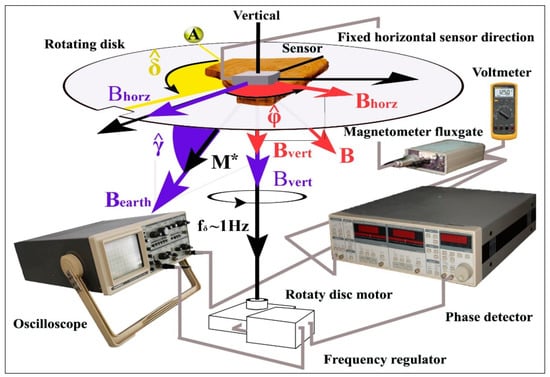
Figure 1.
Illustration of the Earth magnetic field (Bearth) and of the detected projection of the horizontal component (Bhorz) of the fragment field onto the sensor direction during the initial placement of the fragment on the rotating disk. The initial phase angle, δ, of the disk is located between the fixed point, A, of the rotating system and the disk notch. The initial phase angle, φ, of the magnetic field, B, is located between the (fixed) vertical sensor direction and the Bhorz direction, which depends on the fragment placement on the disk.
Accuracy of measurements at a practical level depends: a) on the ability of aligning the x-sensor with respect to the vessel body grooves, which can not be performed with an error less than 1nT. For this reason, measurements on the fragments of the vase body are obtained with a 1nT error (See Supplementary Files), while the maximum sensor accuracy is 0.1–0.2 nT. Therefore, sensors of greater accuracy (eg SQUIDsensors), would not give better results regarding the computation of κ,ω angles, which determine the position of the fragments in the vase bodies. b) on he contact of the fluxgate sensors (of length 3 cm) with the shell surface (see Section 9: Conclusions and Proposals for Future Research), which decreases as their curvature increases.. Thus the precision of the method could be improved or extended to vase fragments of smaller size, using shorter sensors.
For the weak magnetic field extraction from the unwanted lab magnetic background noise the Phase Sensitive Detection (PSD) method [38] was used. The electric signal from the disk rotation, at a certain frequency, f, is used as a reference signal to the phase detector [39]. The direct electric current (1 mV/7 nT) from each fragment, detected by the magnetometer sensor, is converted during the disk rotation into alternating current and used as an input to the phase detector.
The electric signal from the horizontal rotating component, Bhorz, of each fragment is differentiated from the magnetic interferences because it is detected by the phase detector exclusively at the disk rotation frequency, f. If the magnetic field of each fragment displays constant directionality, then its magnitude and initial angular phase difference (δ-φ), are recorded, after the processing of the sinusoidal signals at the phase detector. During the disk rotation, the ceramic material induced magnetization, M*, is oriented perpendicularly to the sensor along the direction of BEarth. Using the PSD method, constant phase differences and weak magnetic fields, with constant directionality and values of a few tens of nT can be found.
After the detection of the fragments magnetic field (Figure 2), the directionality of the base and body in co-belonging fragments is compared. The sensor remains in the same horizontal position, perpendicular to the vertical component and the horizontal component of the geomagnetic field.
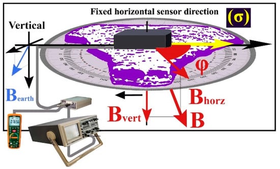
Figure 2.
Illustration of the horizontal component detection apparatus from vase fragments.
During the vase formation at the pottery wheel, circular grooves remain on the fragment surface. Parallel straight lines at an arbitrary direction (σ) are marked on the base fragments (Figure 3a), which suggests their joining direction. Regarding the fragments from the vase bodies (Figure 3b), their direction (σ) is selected along the surface grooves of the pottery wheel.
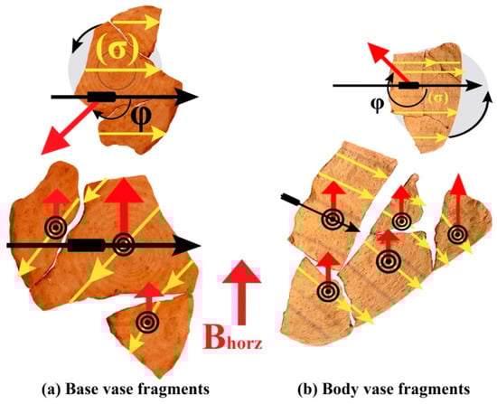
Figure 3.
If the horizontal components of the fragments are positioned such that their vectors are pointing in the same direction, then base fragments and only the neighboring body fragments are oriented such that they join. The distant body fragments are not oriented in a manner that they join.
The fragments are positioned on a leveled angle-measuring apparatus, with the sensor axis aligned along the direction (σ), at a position where Bhorz diverges at an arbitrary angle, φ, from the sensor direction, while the disk is rotated manually until its reading is zeroed. At this position, where Bhorz is vertical to the sensor direction, its direction is marked.
Neighboring fragments are oriented in a joining manner because their magnetic field, acquired before their fracturing, is due to the thermoremanent magnetization along the direction geomagnetic field during their cooling in the kiln.
While finding the joining orientation of the base excavation fragments is not of essential practical value, because it is more easily performed empirically, it can be concluded from the above that neither the magnetic anisotropy of the material nor the irregular fragment shape prevent their joining from the orientation of their magnetic field; in fact this happens with remarkable precision. This is not the case for the distant body fragments, which come in a variety of shapes and are collected in large numbers. This is to be expected, because the thermomagnetic directionality varies depending on the orientation of the vase regions with respect to the geomagnetic field, and it is formed by the rotational symmetry of the ceramic vases.
Fragments from 6 ceramic vases (Figure 4a) are placed on the horizontal angle-measuring apparatus disk, with the marked reference direction (σ) on their surface matching the fixed sensor direction. The component parallel to the fragment surfaces (B//) and the angle of divergence (φ) of the reference direction (σ) with the fixed sensor direction (Figure 5a) are measured at the rotational position where the reading displays its maximal positive value. Representative measurements of the angle φ in body (a) and base fragments (b) of vase 1 are presented in Figure 6.
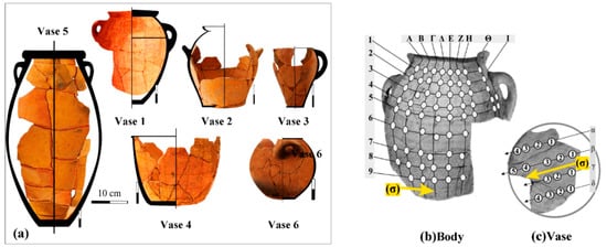
Figure 4.
(a). For the systematic study of the magnetic field directionality, single-sensor measurements from base and body fragments from 6 ceramic vases of the previous two centuries, fired in a traditional kiln, were taken. (b). The body fragments measurements were taken at the vertices of a lattice formed by the grooves, which provide the reference directions (σ), and vertical lines to them. (c). The base fragments measurements are taken on parallel lines, along the arbitrarily chosen joining direction (σ) of the fragments.
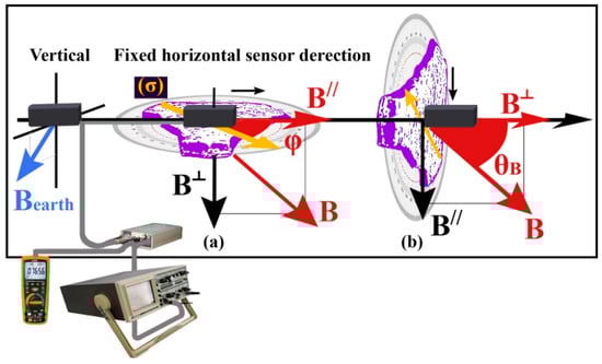
Figure 5.
Illustration of the base and body fragment magnetic field measurement apparatus from the 6 vases, using a sensor that remains perpendicular to the vertical component and the horizontal component of the geomagnetic field, Bearth.
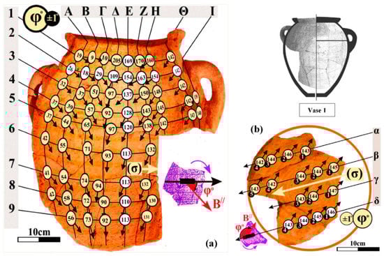
Figure 6.
Representative measurements of the angle φ in body (a) and base fragments (b) of vase 1.
The vertical component (B˪) and its angle (θB) of divergence from the fixed sensor direction (Figure 5b) are measured at the same turning fragments position, albeit on the vertical disk. Representative measurements of the angle θB in body (a) and base fragments (b) of vase 1 are presented in Figure 7.
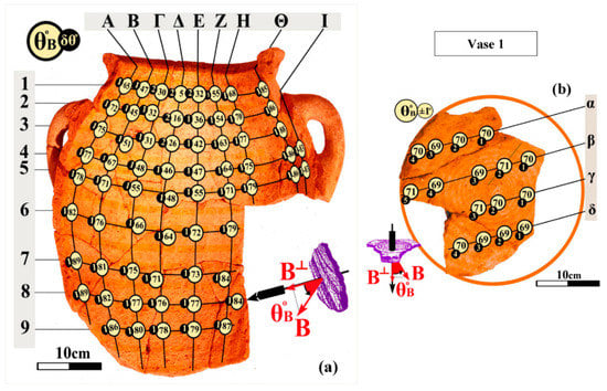
Figure 7.
Representative measurements of the angle θB for body (a) and base fragments (b) of vase 1.
The computed magnitude (Chart 1c), B, and the measured angle, φ (Figure 6b), display similar values only in the co-belonging base fragments of each vase. For the co-belonging body fragments, the magnitude B differs (Chart 1a,b), while the angles φ (Figure 6a), change in a systematic way.
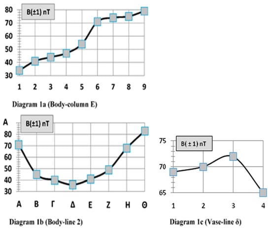
Chart 1.
Representative values of the magnetic field magnitude B computed at body positions (a,b) and base positions (c) of vase 1.
The computed angle θB (Figure 7), displays similar values only for the base fragments of the vases, while it varies in a systematic way for the body fragments.
The measured magnetic field of the co-belonging base fragments by a fluxgate sensor shows similar magnitude and directionality. This is the result of thermoremanent magnetization, which despite the ceramic material magnetic anisotropy, maintains similar magnitude and directionality, because the co-belonging base fragments are composed of the same clay, were fired under the same conditions, at the same time and with a fixed orientation with respect to the earth magnetic field. In any case, local differences are not improbable, which can be due to the incomplete mixture homogenization of clays or eutectic additive materials, temperature variations or kiln aeration and later magnetizations.
The method by which measurements are taken, by fragments placed on the disc in horizontal and vertical positions, due to the time requirements and the required accuracy, is difficult to be used for wide application. The dependence of thermoremanent magnetization in vases shaped in pottery wheels was systematically studied using precise and less tedious magnetic field measurements, by the three fluxgate magnetometer sensors in an orthogonal coordinate system in three dimensions.
3. Magnetic Field Measurements of Ceramic Fragments by 3 Fluxgate Sensors in 3 Orthogonal Axes
The horizontal x-sensor is oriented vertically to the horizontal component and to the vertical component of the earth magnetic field (Figure 8), measured by the y and z-sensors, respectively.
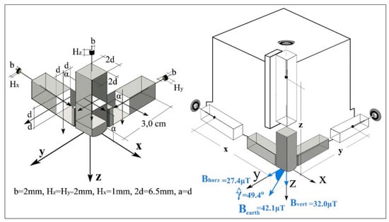
Figure 8.
Illustration of the orthogonal coordinate system in three dimensions of the sensor/magnet apparatus for the compensation of the earth magnetic field and the zeroing of their readings.
The sensor reading (1 mV/7 nT) is zeroed with a maximum precision of 0.01 mV or 0.1 nT by adjusting their axial distance from the Al-Ni-Co type cylindrical magnets (400 KA/m), by turning their mounting screws. The excitation area of each sensor is located on the axis that passes through the center of its square cross section of side 2d = 6.5 mm and at a distance of a = 6.5 mm from its curved edge.
The best, simplest and cost-effective solution is to attach a magnetic field and possible laboratory interference neutralization system to the three-dimensional sensor apparatus. Active shielding could be used, but is not the best choice, from a practical point of view. Within the area of zero magnetic field, the fragments of various sizes should be placed, beside the sensors, and the lifting, leveling and rotation apparatus should be attached. This would require a particularly bulky and complex construction compared to the proposed layout.
Each magnet generates, besides its axial field at the sensor direction, also side fields, which excitate the perpendicular sensors.
The measured axial fields Bzz Byy,Bxx (Figure 9) of the cylindrical magnets, with magnetization M, radius b, and height Hμ, with dipole moment m = M.π.b2.Hμ and at axial distances ξμα from the sensors, are approximated (Table 1) by the formula given in [40] (pp. 394–399):
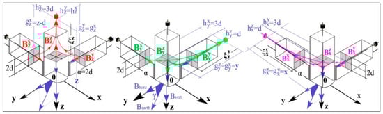
Figure 9.
Illustration of the Earth field, Bearth, and the fields Bμα of the magnets μ = x,y,z at the α = x,y,z sensors.

Table 1.
Computation of the fields at the sensors at the distances x,y,z that zero their readings. The magnetic field is computed at those distances, inside the measurement area. The magnet fields at the sensors and in the measurement area in the Figure 9 and Figure 10 above and in the table are marked with the same color.
The magnet side fields, Bμα≠μ, at axial distances gμα≠μ and side distances from the sensors, hμα≠μ, are approximated by the formula:
The summed components of the field Bμδ of the μ=x,y,z magnets and the earth field components at the axial distances δ=x,y,z where the sensor readings become zero (Figure 10a), are approximated [40], at the measurement area, by the formulas:
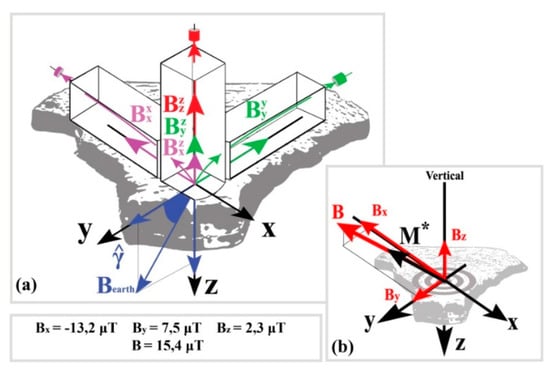
Figure 10.
Illustration, (a) of the individual fields, Bμδ of the μ = x,y,z magnets at axial distance δ = x,y,z, and of the earth and (b) of the total field inside the measurement area, along the direction of which the induced magnetization M* of the ceramic material is oriented.
All the following measurements are taken at the same fixed position with respect to the geomagnetic field by the sensor/magnet apparatus forming a three-dimensional orthogonal system. The induced-magnetization contribution of the ceramic material along M*(Figure 10b) to the sensor readings is checked in the following experiment by comparing the measurements (Appendix B.2) taken inside a null magnetic field.
4. Experimental Results: Modelling the Ceramic Region generating the Magnetic Field detected by the Sensors for the Calculation of Magnetization in Base Vase Specimens
The remanent magnetization dependence and computation on the magnetic sensor measurements, is studied in Appendix B through a series of experiments (Appendix B.1, Appendix B.2, Appendix B.3, Appendix B.4 and Appendix B.5) in irregular base fragments (Appendix B.1) and mainly in cylindrical specimens (Appendix B.2, Appendix B.3, Appendix B.4 and Appendix B.5) from the base of vases 4–6 (Figure 4a).
The angles, θB, γ > θB, between the field, B, and the magnetization, M, increase as the distance to the measurement position from the edge of the fragment decreases.
From the experimental results of the measurements on specimens and fragments from the base vases 4–6, it is found that:
- The sensors detect the axial field B at the edge of a cylindrical region of ceramic material (Appendix B.1, Appendix B.2 and Appendix B.5) in the direction of the remanent magnetization, M.
- The measured magnetic field is only due to the remanent magnetization of the ceramic material (Appendix B.2), and it is not altered by its induced magnetization.
- The height, ℓ, of the magnetically detecting area of the ceramic material by the sensors (Appendix B.2, Appendix B.3, Appendix B.4, Appendix B.5 and Appendix B.7), depends of the angle, γ, between the magnetization M and the vertical z-axis on specimens’ surface, each specimen thickness, L, and the distance, D, between the sensors and the fragment edge along Bxy, when the vertical z-sensor reading is doubled:
- When D > d = L.tanθB the height, ℓ = L/cosθB, depends on the thickness, L, of the fragment.
- When D < d the height, ℓ =D/sinθB is dependent on the distance D.
- The radii (Appendix B.5), ri = 2αi.cosγ (i = ˪,//), of the ceramic cylindrical areas depends on the directionality (γ) of magnetization and of the parameters α˪,α//, which, geometrically, are the sensitivity radius of sensors around the measurement position of the vertical and the parallel sensors, respectively.
The field flow in the excitation coil of the vertical sensor, Bi˪ (i = xy,z), is smaller than that of the parallel (Bi// ≈ λ.Bi˪) sensor, for the measurement of the same component Bi of the field. The normalization factor λ ≈ 2, for the correction of their readings (Appendix B.5), has a similar value in non co-belonging fragments with different magnetization M due to the different orientation of the excitation coils on the specimen surface. The radii α˪, α// increase with the magnetization magnitude, M, increase and display similar values in co-belonging shells.
- •
- The sensor readings display similar values when the ratios r/ℓ, of the cylindrical detecting areas of the ceramic material by the sensors, as does the measured axial field at the end of the solenoids with the same current and number of spirals, where the ratio of the radius, r, to their height, ℓ, is kept constant. The measured magnetic field B of the ceramic cylindrical areas is approximated by the magnetic field of a solenoid with the same dimensions.
- -
- If D ≥ d = L.tanγ (Figure 11a), the height, ℓ = L/cosγ, depends on the thickness, L, of the fragment and the components, Mi (i = xy,z), are approximated by the sufficient length relationships:
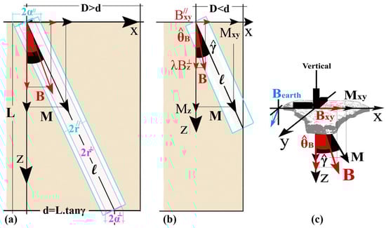 Figure 11. Illustration of the ceramic cylindrical areaof the material that generates the magnetic field detected by the vertical (a) and parallel (b) sensor depending on the distance, D, between the sensors position and the edge of the specimen. The x-sensor (c), remains perpendicular to the vertical and the horizontal components of the geomagnetic field. The measurements are taken along Bxy, which is oriented in the direction of the x-sensor.
 - -
- If D ≤ d (Figure 11b), the height ℓ=D/sinθ depends on the distance, D, of the measurement position from the fragment edge in the magnetization direction, M. The components Mi (i = xy,z) are approximated by the insufficient length relationships:
Since αxy//>αz˪, the computed deviation, θB, of the field from the vertical (Figure 11c) at the measurement is less than the angle γ of the magnetization M.
The horizontal components, Bxy, Mxy, of the measured field, B, and magnetization, M, diverge at the same angle φ from the horizontal direction of the x-sensor.
The quantities λ, α˪, α//, γ, M, Mi, (i = xy,z) were calculated with remarkable accuracy using the above relationships from the sensor readings and also by the thickness, L, and distance, D, measurements (Appendix B.6) in base specimens of vases 4 and 6.
5. Computation of Magnetization in Irregular Fragments of the Vase Base 1, 2 & 3
The components, Mz, Mxy, angle γ of the magnetization M, and sensitivity radii of the sensors, α˪, α//, in fragments from the bases of vases 1, 2 and 3 (Figure 4a) are computed by the same using way (Appendix B.7) in specimens from base of vases 4, 5 and 6, without any need for cutting specimens.
The three-dimensional orthogonal system apparatus of sensors/magnets remains in the same position with respect to the earth magnetic field (Figure 12), with the x-sensor oriented perpendicularly (By = 0, Bx = Bxy > 0) to the horizontal and vertical component of the geomagnetic field.
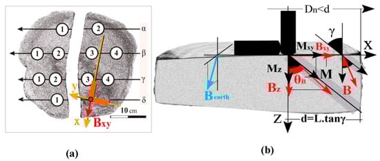
Figure 12.
Illustration of the measurement methodology (b) of the magnetization components, Mi (i = xy,z), and the sensitivity radii of the vertical, αz˪, and parallel sensor, αxy//, in a base fragment (a) of vase 2.
The measurements of Bxy, Bz are taken on Bxy in the direction of the x-sensor from the measurement position where the systematic reduction in the magnetic field readings begins at measured distances Dn < d = L.tanγ from the fragments’ edge.
The computation of sensor magnetization components, Mi (i = xy,z), and sensitivity radii, αz˪,αxy//, from the field measurements, Bi (i = xy,z), is performed using the least squares method (Appendix A), from the equation:
The measurement results are presented in Appendix B.7.
6. Aggregate Results and Conclusions of Calculating Magnetization from Magnetic Field Measurements on Samples and Fragments of the Base of Vases 1–6
The measured components of the magnetic field, Bi (i = xy,z), depend on the directionality (γ), magnetization magnitude M, and thickness, as well as the position and orientation of the sensors on the surface of the fragments. From the above perspective, the normalization constant, λ, the sensitivity radius of sensors α˪, α//, of the vertical and parallel sensors around measurement position, Bi, and the magnetization (Mi, M, γ) in irregular base fragments of the vases 1, 2 and 3 (Appendix B.6) and in base samples of vases 4, 5 and 6 (Appendix B.7) are computed.
The sensitivity radii, α˪, α//, increase with the increase of the magnetization magnitude (Chart 2) and differ (Table 2) in base fragments from different vases. Since αxy//>αz˪, according to the relationships (4,5), the computed deviation, θB, of the field from the vertical (Figure 13) at the measurement position is less than the angle γ of the magnetization M. Since αx//= αy//, the horizontal components, Bxy, Mxy, of the measured field, B, and magnetization, M, diverge at the same angle φ from the horizontal direction of the x-sensor. For this reason, the co-belonging base fragments or the adjacent body fragments of the vases are oriented in such a way that they join (Section 2), when the Bxy are placed in parallel directions.
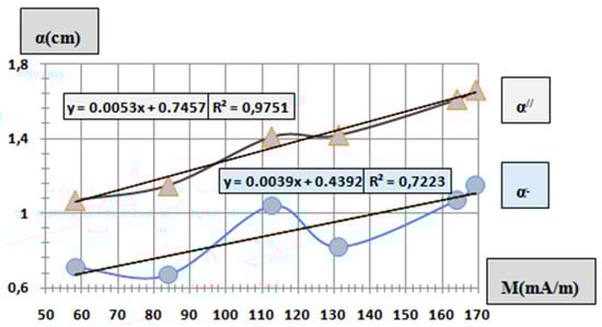
Chart 2.
Change of the sensitivity radii of the vertical α˪ and parallel sensor as a function of the computed magnetization magnitude, M, in the base fragments from the vases 1–6. While the number of points in the graph is not sufficient, their change appears linear, with a similar slope.
Table 2.
Computation of the magnitude, M, of the magnetization directionality (γ) and of the normalization constants, λ, α˪, α//, of the sensor readings in irregular base fragments of the vases 1, 2 and 3 and in base specimens of the vases 4, 5 and 6.
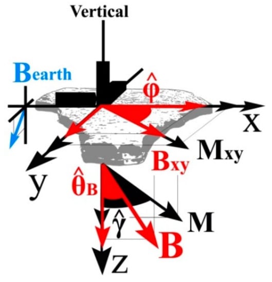
Figure 13.
The magnetization, M, and the magnetic field, B, diverge at the same angle, φ, from the horizontal x-axis, while the angles, θB, γ > θB, between the field, B, and the magnetization, M, deviate as the distance to the measurement position from the edge of the fragment decreases.
With the proposed perspective of the sensors’ mode, the ceramic area that generates the magnetic field, which is detected by the sensors and the normalization constants (λ, α˪, α//) of their readings from measurements of the magnetic field in base vase fragments, the magnetization of co-belonging body fragments of vases 1–6 is computed.
7. Computation of Magnetization in Body Fragments from Vases 1–6
Measurements by the three-dimensional orthogonal system of sensors/magnet apparatus are taken in the same position, with the x-sensor oriented perpendicularly to the horizontal and vertical component of the geomagnetic field. The measurement positions are situated at the edges of a mesh formed from lines vertical to the traces of the grooves from the formation of the six vases (Figure 4b) on a pottery wheel. To exploit the rotational symmetry of vases (Figure 14a), the measurements are taken with respect to a right-hand coordinate system, with the x-axis along the groove direction, the y-axis perpendicular to the surface and pointing towards the inside of the fragments, and the z-axis pointing towards the base of the vases.
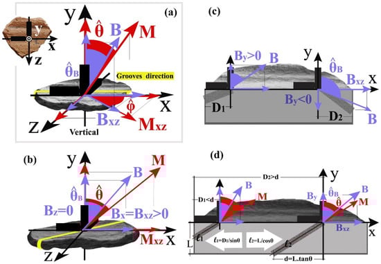
Figure 14.
Methodology for calculating the components of the magnetization M from the measured components of the magnetic field B in the considered reference system.
The components Mi (i = x, y, z) are computed from the measurements Bi of the field, in the rotating position where the grooves are oriented in the direction of the x-sensor.
The components of the measured field, B, and of the magnetization, M, in the considered coordinate system (Figure 14a) are computed by the relations:
Bx = B. sinθB. cosφ, By = B.sinθB.sinφ, Bz = B.cosθB, Mx = M. sinθ.cosφ, My = M.sinθ. sinφ, Mz = M.cosθ
To determine the deviation, θ, of the magnetization from the vertical (Figure 14b), measurements of the Bxz, By are taken, by rotating the fragments at an angle φB = φ and orienting Bxz in the x-direction, in the position where Bz = 0 and Bxz > 0.
The distance, D, between the measurement position and the fragment edge in the common direction of the Mxz,Bxz (Figure 14c) is measured in the negative or positive x-semi-axis, when By > 0 or By < 0.
The distance D (Figure 14d) may be sufficient (D > d = L.|tanθ|) or insufficient (D < d), for the measured fragment thickness, L, at the measurement position. In any case, the magnetization angles θ = θD or θ = θL are approximated [41] by the solution of the 3rd degree equations (using the Newton-Raphson method):
The constants αxz//,αy˪, λ are computed (Table 2) from the field measurements in co-belonging base fragments of the vases:
- -
- If θL > θD, then D > d = L.tanθL and θ = θL. For the computation of the components of the magnetization, M, the sufficient length Equations (4) are used.
- -
- -If θL < θD, then D < d = L.tanθD and θ = θD. For the computation of the components of the magnetization, M, the insufficient length Equations (5) are used.
Experimental results (analytical results at each calculation stage of magnetization are presented in “Supplementary Files” for the body of vase 6. For the reproducibility of the results, the magnetic field measurements for the remaining vases in each position of their body are listed therein) show that the computed magnitude, M, displays similar values in the base and body fragments, which is a criterion for finding ceramic fragments of the same vase from archaeological excavations. The angles, θ, φ, change in a systematic way because their values are dictated by the rotational symmetry of the vase. This is confirmed in the next section, where the position of fragments in the bodies of 6 vases is identified by successive transformations of magnetization components.
8. Position Localization of Fragments in the Body of a Vase from the Directivity of the Remanent Magnetization
If γearth is the inclination and ξ the declination of the local magnetic field of the Earth (BEarth) during pottery firing (Figure 15), then its components with respect to the right-hand axial coordinate system, XYZ, of the vase, where the Z-axis of rotational symmetry of the vase deviates from the vertical at α deviation angle,α, of the vase on the kiln floor and points towards its base, are computed by the equations:
BXEarth = BEarth. sinγ. cosξ, BΥearth = Bearth.sinγ. sinξ, BZEarth = Bearth. cosγ, γ =(90° − γEarth) ± α
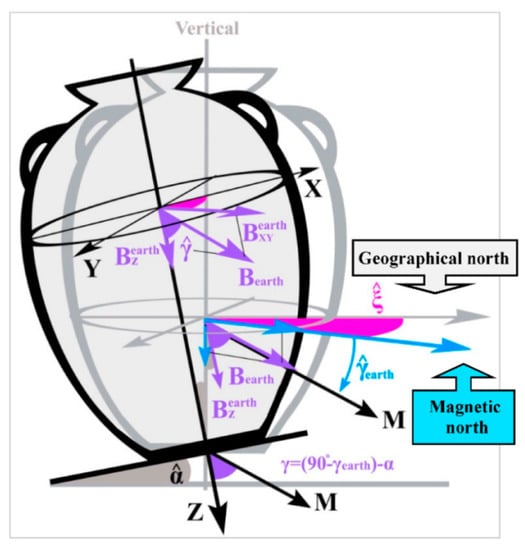
Figure 15.
Illustration of the geomagnetic field,Bearth, during firing of a vase with rotational symmetry with respect to the right-hand axial reference system XYZ where the Z-axis coincides with the axis of rotational symmetry and points towards the vase base.
The declination, ξ, of the geomagnetic field cannot be computed without knowing the vase orientation in the kiln. The inclination, γearth, of the geomagnetic field cannot be computed without knowing the deviation angle, α, of the kiln with respect to the horizontal plane.
The circular grooves in the vase body, which are parallel to its base, deviate from the horizontal plane according to the same angle, α, due to the rotational symmetry of the base. In any vase with rotational symmetry, and for any considered axial reference system where the z-axis coincides with the axis of rotation, the X,Y axes are defined on the plane of the same transverse groove on the vessel body.
The angle, γ, of inclination of the geomagnetic field from the vase axis of symmetry, is equal to the deviation angle of magnetization, M, calculated from measurements of the magnetic field of base fragments (Appendix B.6 and Appendix B.7) since the ceramic material magnetization obtains the orientation of the geomagnetic field during firing.
8.1. Formation of Remanent Magnetization in Vases with Cylindrical Symmetry
Measurements of the field (Figure 16a), B, are obtained in right-hand reference systems (xyz)*, where the x*-axis has the direction of the transverse grooves, the y*axis passes through the axis of rotational symmetry and the z-axis is tangential to the side walls, directed towards the vase base.
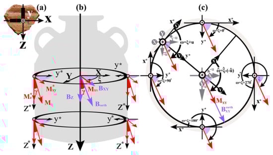
Figure 16.
Direction of the sensors (a) in relation to the grooves of vase body fragments. Illustration of the magnetization, M, of ceramic material along the direction of the geomagnetic field, Bearth, during firing of a vase with rotational symmetry in right-hand reference systems, (xyz)*, along longitudinal (b) and transverse cross-sections (c) of the vase body.
In the specific case of vases with cylindrical symmetry, because the z*-axis in the measurement system of the B field is parallel to the axis of symmetry, Z, (Figure 16b) the position of each longitudinal axial section is defined by the rotation angle, u, of the right-hand axial reference system, XYZ, of the cylindrical vase (Figure 16c), around the Z-axis of rotational symmetry.
Since magnetization, M, obtains the orientation of Bearth in the pottery kiln, then for every rotation angle, u, of the axial reference system, XYZ, the M-magnetization components at the fringe of each transverse groove are determined by the rotation transformation of the peripheral reference systems (xyz)* at an angle ω = ξ − u around the z*-axis:
where: ω = ξ − u, γ = (90° – γEarth) ± α
Mx* = M·sinγ·cosω = Mxy*· cosω, My* = M· sinγ·sinω = Mxy*· sinω, Mz* = M·cosγ
Although the angles u, ξ cannot be determined without knowing the orientation of the vase in the pottery kiln, the angle ω = ξ – u is determined by calculating the magnetization of the fragments of the vase body.
8.2. Formulation of Remanent Magnetization in Vases with Arbitrary Rotational Symmetry
In the general case of vases with arbitrary rotational symmetry (Figure 17a), the side walls diverge at different angles, κ, from the axis of symmetry in each longitudinal section, (α,β,γ,δ), of the vase and at the same angle κ in each transverse groove, (1,2,3).
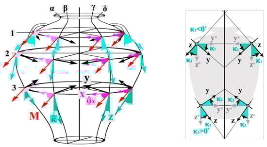
Figure 17.
(a). Illustration of the reference systems (xyz) where the magnetic field measurements are taken, in transverse and longitudinal sections of a vase body with arbitrary rotational symmetry. The angles, φx, of magnetization, M, with the x-axes oriented in the direction of the grooves maintain a constant value along each longitudinal section (1,2,3) and vary along each cross-section (α, β, γ, δ) of the vase. The angles, κ, between the vertical z-axes in the grooves and the axis of rotational symmetry maintain a constant value along each transverse groove and vary along each longitudinal section (α,β,γ,δ) of the vase. The vertical y-axes on the surface of the fragments pass through the axis of rotational symmetry of the vase. (b). The magnetization components in the reference systems (xyz), where the magnetic field measurements in vase fragments with arbitrary rotational symmetry are taken, are derived from a rotational transformation of the reference systems (xyz)* of the cylindrical vase at an angle of inclination κ around the x*-axes.
The components Mi (i = x,y,z) in the reference systems (xyz) of the Bi field measurements (Figure 18) are derived from a rotational transformation (Figure 17b) of the reference systems (xyz)* of the cylindrical vase at an inclination angle κ around the x*-axes:
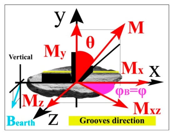
Figure 18.
Illustration of magnetization components in the body fragment reference system of a vase whose magnetic field measurements are taken, and computed by the equations: Mx = M. sinθ.cosφ, My = M.sinθ. sinφ, Mz = M.cosθ. The magnetization, M, and the magnetic field, B, diverge at the same angle, φ = φB, from the horizontal x-axis.
❖ Based on the above transformation, the circumferential position of the fragments in each cross section of the vase is determined by the angle ω,which is computed by the formula:
The angles , are calculated from the magnetic field measurements of the body fragments, while the angle γ is calculated from the magnetic field measurements in co-belonging fragments of the vase base.
❖ The height-position of the fragments in each longitudinal section of the vase is determined by the inclination, κ, which is computed by the equation:
Determining the change in directionality of remanent magnetization, M, in the vase body in a manner dictated by its rotational symmetry, is performed from the calculated angles ω, κ at each measurement position, using the inverse rotational transform of the calculated magnetization components at an angle -κ around the x-axis (Figure 19a), from the reference system (xyz), where the magnetic field measurements are taken, to the (xyz)* reference system (Figure 19b) of the cylindrical vase:
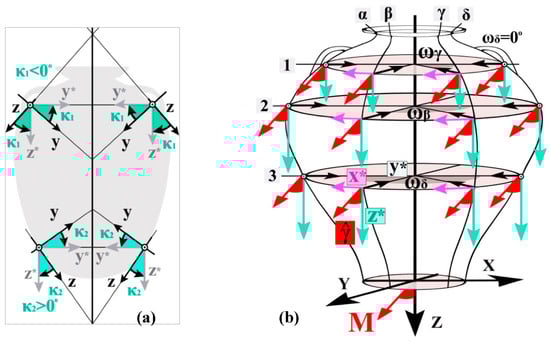
Figure 19.
(a). Illustration of the inverse transformation at an angle -κ around the x-axes, from the reference systems (xyz), where the magnetic field measurements are taken, to the reference systems (xyz)*of the cylindrical vase. (b). Visualization of reference systems, (xyz)*, of the cylindrical vase, in a vase with arbitrary rotational symmetry.
In the reverse transformation (Figure 19b), the components Mx*,My* and the angle ω should display similar values in each longitudinal section of the body, based on the above equations, while Mz*, which depends only on angle γ, should display similar values in each measurement position. Indicative experimental results with the reverse transformation are given from measurements of body fragments (Table 3) from vase 6.
Table 3.
Indicative values of the transformed components, Mi* (i = xyz), of magnetization in the reference systems (xyz)* of the cylindrical vase, in fragments of the body (a) and the base (b) from vase 6. The values inside the colored frames computed by the insufficient length (5) relationships.
The components Mx*,My* and the angle ω display similar values (Table 3a) in each longitudinal section of the body. Inclination, κ, displays similar values in each transverse groove of the vase.
Mz* displays similar values (Table 3b) in each measurement position and with that which computed for the base fragments of the vase.
8.3. Experimental Results: Screening of Co-Belonging Fragments and Determination of Their Position in the Body of a Vase from Their Magnetization
The computed values for the inclination, κ, and the angle ω are displayed (Figure 20, Figure 21, Figure 22, Figure 23, Figure 24, Figure 25, Figure 26, Figure 27, Figure 28, Figure 29, Figure 30 and Figure 31) on the bodies of the six vases. The magnetization magnitude M (mA/m) in body fragments displays similar values (Table 4, Table 5, Table 6, Table 7, Table 8 and Table 9), and with those calculated from the base fragments of the vases.
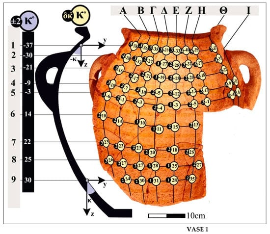
Figure 20.
Angles, κ, display similar values in each transverse groove of the body vase 1. The computed values for the inclination, κ, from the sensor readings are similar to the measured ones.

Figure 21.
Angles, ω, display similar values in each longitudinal section of vase 1. If the common direction of the transformed components, Mxy*, in each longitudinal section of body fragments, is aligned along the common direction of the components, Mxy, of base fragments, then the body and the base are oriented such that they join.
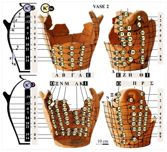
Figure 22.
Angles, κ, display similar values in each transverse groove of body vase 2. The computed values for inclination, κ, from the sensor readings are similar to the measured ones.
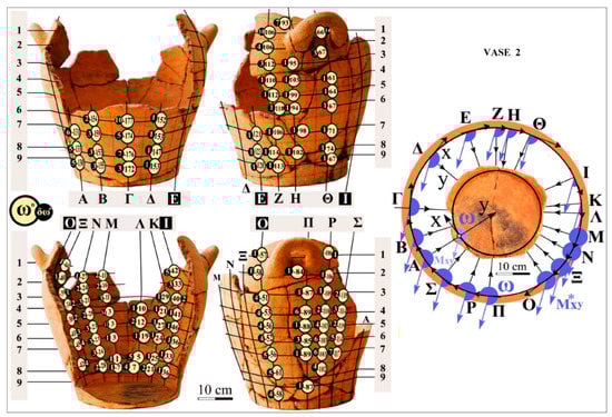
Figure 23.
Angles, ω, display similar values in each longitudinal section of vase 2. If the common direction of the transformed components, Mxy*, in each longitudinal section of body fragments, is aligned along the common direction of the components, Mxy, in base fragments, then the body and the base oriented such that they join.
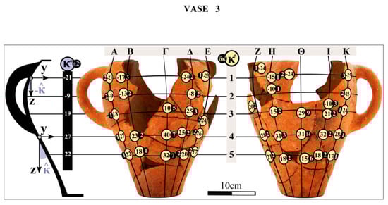
Figure 24.
Angles, κ, display similar values in each transverse groove of the body vase 3. The computed values for inclination, κ, from the sensor readings are similar to the measured ones.
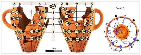
Figure 25.
Angles, ω, display similar values in each longitudinal section of vase 3. If the common direction of the transformed components, Mxy*, in each longitudinal section of body fragments, is aligned along the common direction of the components, Mxy, in base fragments, then the body and the base are oriented such that they join.
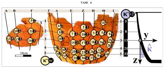
Figure 26.
Angles, κ, display similar values in each transverse groove of the body vase 4. The computed values for inclination, κ, from the sensor readings are similar to the measured ones.
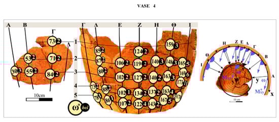
Figure 27.
Angles, ω, display similar values in each longitudinal section of vase 4. If the common direction of the transformed components, Mxy*, in each longitudinal section of body fragments, is aligned along the common direction of the components, Mxy, in base fragments, then the body and the base are oriented such that they join.
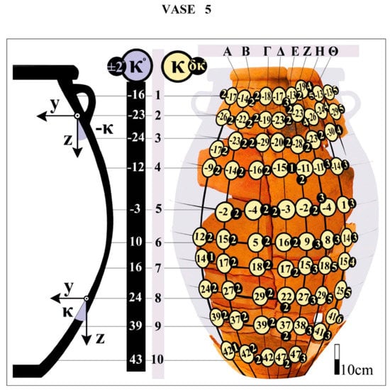
Figure 28.
Angles, κ, display similar values in each traverse groove of the body vase 5. The computed values for inclination, κ, from the sensor readings are similar to the measured ones.
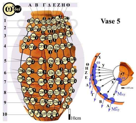
Figure 29.
Angles, ω, display similar values in each longitudinal section of vase 5. If the common direction of the transformed components, Mxy*, in each longitudinal section of body fragments, is aligned along the common direction of the components, Mxy, in base fragments, then the body and the base are oriented such that they join.
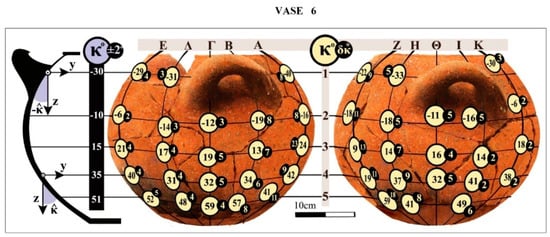
Figure 30.
Angles, κ, display similar values in each transverse groove of the body vase 6. The computed values for inclination, κ, from the sensor readings are similar to the measured ones.
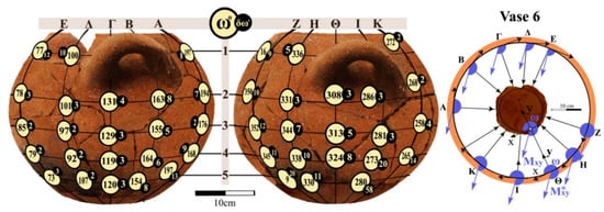
Figure 31.
Angles, ω, display similar values in each longitudinal section of vase 6. If the common direction of the transformed components, Mxy*, in each longitudinal section of body fragments, is aligned along the common direction of the components, Mxy, in base fragments, then the body and the base are oriented such that they join.
Table 4.
The magnetization magnitude in body and vase fragments of vase 1 display similar values. The values inside the colored frames computed by the insufficient length relationships (5).
Table 5.
The magnetization magnitude, M, in body and vase fragments of vase 2 display similar values. The values inside the colored frames computed by the insufficient length relationships (5).
Table 6.
The magnetization magnitude in body and base fragments of vase 3 display similar values. The values inside the colored frames are computed by the insufficient length relationships(5).
Table 7.
The magnetization magnitude in body and vase fragments of vase 4 display similar values. The values inside the colored frames are computed by the insufficient length relationships (5).
Table 8.
The magnetization magnitude in body and vase fragments of vase 5 display similar values. The values inside the colored frames are computed by the insufficient length relationships (5).
Table 9.
The magnetization magnitude in body and base fragments of vase 6 display similar values. The values inside the colored frames are computed by the insufficient length relationships (5).
The slope, κ (Figure 20, Figure 22, Figure 24, Figure 26, Figure 28 and Figure 30) which displays similar values in each cross-section and determines the height-position of the fragments, is compared with the measured inclination of the walls with respect to the axis of symmetry in each vase. The computed values for the inclination, κ, from the sensor readings are similar to the measured ones.
The angle ω (Figure 21, Figure 23, Figure 25, Figure 27, Figure 29 and Figure 31) displays a similar value in each longitudinal section and varies at the transverse measurement positions, defining the peripheral position of the fragments on the body of each vase.
From the orientation (ω) of the transformed Mxψ* in the vessel body and of Mxψ in the fragments of the base (Figure 21, Figure 23, Figure 25, Figure 27, Figure 29 and Figure 31), the jointing position of the base and the body of each vase is determined. The shape of the original vase can be reconstructed when only a few non adjacent fragments are available.
9. Conclusions and Proposals for Future Research
From the experimental results it can be seen that despite the small range of the magnetization magnitude in the six vases, the screening of excavation fragments can be done on the basis of their similar magnetization values. The position of co-belonging body fragments of the vases is determined with satisfactory precision by calculating the angles ω, κ.
The laboratory environment in which the proposed device is intended to be used is a large space, in which the vase fragments of each excavation layer are placed on platforms and separated into the excavated squares in which they were found. From each excavation block the characteristic fragments belonging to the bases, the orifices or handles of the vases and the fragments with written or embossed decoration are separated. The characteristic fragments determine the number of surviving vases and the search for co-belonging shells, which, in the simplest case, are located in adjacent excavated squares. In the common cases of perturbed excavation layers due to natural phenomena (such as floods) or illegal excavations, the procedure is more difficult, because the co-belonging fragments must be sought in the excavation layers above or below, in each excavation square, or in remote excavation squares. The positioning of the fragments in adjacent excavation layers and squares is of critical importance for the finding of co-belonging fragments. The investigation and screening of co-belonging fragments is performed by conservators.
The apparatus is not recommended to be used with fragments of characteristic portions of the vases (nozzles, handles), with fragments with written or embossed decoration, because it is easier for them to be located in an empirical manner.
Small vases of daily use (e.g., plates, cups), without characteristic portions on their surface may have been manufactured from the same clay and fired in the same kiln under the same conditions. In that case the co-belonging vase fragments cannot be distinguished from the magnitude of thermoremanent magnetization, because it displays similar values. This is a very useful information on their manufacturing technique and on the origin of the raw material. The fragments from each vase can be distinguished from their different magnetization directivity at the assembly stage. The method is ineffective in the rather rare case of vases of the same size and shape from the same clay, placed in the same orientation in the kiln, relative to the Earth’s magnetic field.
It should be noted that the position of small vase fragments with high curvature is hampered, at least with the ~3 cm fluxgate sensors used in this research. The error in calculating the angles ω, κ increases as the sensor contact with the fragment surface becomes smaller. Magnetic field measurements in larger curvature fragments can be performed with shorter-length sensors.
However, in any case, it is a small number of fragments with characteristic curvature, which are easier to categorize and assemble empirically.
The apparatus is recommented to be used for the location and assembly of unidentified fragments from medium-size vases (basins, hydries) or larger-size (usually pithos vases), which are the most common excavation findings.
In medium-size vases, which display a variety of shapes due to their different uses, the risk of deformation during drying is minimized with the admixture of aggregates, depending on their shape and size. The possibility of finding medium sized pots of the same clay fired in the same kiln in the same excavation layer is small. In the event that the measured magnitude shows similar values, the above applies.
Regarding large size vases for storage use, these were fired in one-use kilns built around the vase, from antiquity to today. Therefore the possibility of two large vases from the same clay to have been fired in the same kiln is very small.
The methodology can be used to screen fragments from archaeological excavations under the following conditions:
- -
- Finding co-belonging fragments of the vase base is essential for calculating the magnetization deviation angle, γ, and the parameters α˪, α//, λ from measurements of their magnetic field. This is not a problem, because in the usual process of screening co-belonging fragments, the base fragments, which are easily identified, are initially collected and the neighboring fragments of the vase body are then searched.
- -
- In the fragment reference system, where measurements are taken, the x-axis is oriented in the direction of the vase grooves while the y-axis is perpendicular to the surface and directed towards the inside of the fragments. To take measurements on all fragments in relation to the same reference system, the z-axis must be oriented towards the base (or the aperture) of the vase. The orientation of each fragment with respect to the base or the aperture of the vase can be done easily, on the basis of its shape and the curvature of the grooves on its surface.
Proposals for future research, based on additional preliminary investigations, are given below.
1) Experimental application of the method in fragments from archaeological excavations.
2) Construction of ceramic specimens from different raw materials and with different granulometry, fired in the same pottery kiln under different slopes of the kiln floor.
- -
- Construction of ceramic specimens from the same raw material, fired in the same kiln, with the same slope, but under different oxidative conditions and at different temperatures.
- -
- Analysis of the composition of the specimens and their content in magnetic oxides.
The above are necessary in order to study the dependence of remanent magnetization on the clay composition, the temperature/ventilation conditions in the pottery kiln, the orientation of the geomagnetic field, and the degree of magnetic anisotropy of the ceramic material. For the above research a traditional wood kiln is required. In ceramic specimens made from different commercially available clays fired in an electric kiln, the measured magnetic field was less than 10nT and without clear orientation, as a result of magnetic fields from the electric currents of the kiln.
3) Investigation of the sensitivity radii dependence of the vertical (α˪) and parallel (α//) sensors on the magnetization magnitude of the ceramic material.
- -
- -Investigation of the mode, the sensors’ degree of excitation, and of the dependence of the normalization constant, λ, of the vertical and parallel sensor readings as well as of α˪, α//, on measurements of the same specimens at different distances from their surface. A prerequisite for these are magnetic field measurements in ceramic materials with higher thermoremanent magnetization, so that their magnetic field is attenuated at longer distances from their surface.
- -
- Investigation of the dependence of the normalization constant, λ, of the vertical and parallel sensor readings and their correlation with the dimensions and technical characteristics of the sensors from measurements of the same specimens with different types of fluxgate sensors.
4) Investigation of the feasibility of constructing a handy three-sensor fluxgate magnetometer for local measurements of weak surface fields (1–1000 nT) in ceramic materials with a magnetization of 1–1000 mA/m for archaeological use.
5) Investigation of induced magnetization of ceramic materials in alternating magnetic fields as an additional criterion for the screening of co-belonging excavation fragments.
Experiments were carried out by the successive placement of cylindrical ceramic specimens from co-belonging vase fragments at specific locations inside a solenoid (L~3 mH) in an RLC circuit in a field (~50 μΤ), and the induced magnetization was calculated by increasing the inductance of the coil at the resonance frequency [34] (pp. 21–34) of the circuit (Null Detection technique). In sequential addition of co-belonging tiles at different resonance frequencies (f = 40–95 KHz), similar increase in their induced magnetization was observed, which is a criterion for distinguishing samples from different vases.
- -
- Investigation of the possibility of constructing a handy instrument for local surface measurements of induced magnetization of ceramic materials from an alternating magnetic field for archaeological use for the purpose of screening the co-belonging excavation fragments.
6) Investigation of the application of the method in rocks with remanent magnetization, for the localization of changes in local soil morphology, by comparing the orientation of the magnetic field of the parent rock and its detached parts. Experiments were conducted in fragments from serpentinite and were found to be oriented in a joining manner, from their thermoremanent magnetization.
These studies will be presented in follow up publications in the near future.
Supplementary Materials
The following are available online at https://www.mdpi.com/2076-3417/9/16/3310/s1, Table S1: Measurements D, L, and sensor readings of Bi (i = xz,y), with the x-sensor aligned along the common direction of Bxz, Mxz, on the body fragments of vase 6. Table S2: Computation of the angles θ, of the distances d, and of the magnetization components My, Mxz, from the field components, By, Bxz, with the x-sensor axis aligned along the common direction of Bxz, Mxz. The values inside the colored frames (D<d=L.tanθ) are computed using the sufficient length relationships (4). Table S3. Sensor readings with the x-sensor oriented in the grooves’ direction on the body fragments of vase 6. Table S4. Computation of the magnetization components, Mi (i = x,y,z), of the magnitude M and of the angles θ,φ, from sensor readings with the x-sensor oriented in the grooves direction in body fragments of vase 6. Table S5a. Measurements D, L, and sensor readings of Bi (i = xz,y), with the x-sensor aligned along the common direction of Bxz, Mxz, on the body fragments of vase 1. Table S5b. Measurements D, L, and sensor readings of Bi (i = xz,y), with the x-sensor aligned along the common direction of Bxz, Mxz, on the body fragments of vase 1. Table S6a. Sensor readings of Bi (i = x,y,z), with the x-sensor oriented in the grooves’ direction on the body fragments of vase 1. Table S6b. Indicative sensor readings of Bi (i = x,y,z), with the x-sensor oriented in the grooves’ direction on the body fragments of vase 1. Table S7a. Measurements D, L, and sensor readings of Bi (i = xz,y), with the x-sensor aligned along the common direction of Bxz, Mxz, on the body fragments of vase 2. Table S7b. Measurements D, L, and sensor readings of Bi (i = xz,y), with the x-sensor aligned along the common direction of Bxz, Mxz, on the body fragments of vase 2. Table S7c. Measurements D, L, and sensor readings of Bi (i = xz,y), with the x-sensor aligned along the common direction of Bxz, Mxz, on the body fragments of vase 2. Table S7d. Measurements D, L, and sensor readings of Bi (i = xz,y), with the x-sensor aligned along the common direction of Bxz, Mxz, on the body fragments of vase 2. Table S8a. Indicative sensor readings with the x-sensor oriented in the grooves’ direction on the body fragments of vase 2. Table S8b. Indicative sensor readings with the x-sensor oriented in the grooves’ direction on the body fragments of vase 2. Table S8c. Indicative sensor readings with the x-sensor oriented in the grooves’ direction on the body fragments of vase 2. Table S8d. Indicative sensor readings with the x-sensor oriented in the grooves’ direction on the body fragments of vase 2. Table S9. Measurements D, L, and sensor readings of Bi (i = xz,y), with the x-sensor aligned along the common direction of Bxz, Mxz, on the body fragments of vase 3. Table S10. Indicative sensor readings with the x-sensor oriented in the grooves’ direction on the body fragments of vase 3. Table S11. Measurements D, L, and sensor readings of Bi (i = xz,y), with the x-sensor aligned along the common direction of Bxz, Mxz, on the body fragments of vase 4. Table S12. Indicative sensor readings with the x-sensor oriented in the grooves’ direction on the body fragments of vase 4. Table S13a. Measurements D, L, and sensor readings of Bi (i = xz,y), with the x-sensor aligned along the common direction of Bxz, Mxz, on the body fragments of vase 5. Table S13b. Measurements D, L, and sensor readings of Bi (i = xz,y), with the x-sensor aligned along the common direction of Bxz, Mxz, on the body fragments of vase 5. Table S14a. Indicative sensor readings with the x-sensor oriented in the grooves’ direction on the body fragments of vase 5. Table S14b. Indicative sensor readings with the x-sensor oriented in the grooves’ direction on the body fragments of vase 5.
Author Contributions
M.N. formulated the research goals and aims, the development of methodology, the investigation process, the visualization and the writing of the published work. A.P. has co-supervised the work, provided the instrumentation and contributed to the investigation, methodology and project administration, to the validation of experiments, the visualization of data and to the critical review of the publication. T.M. and A.V. have co-supervised the work. They contributed to the validation of the work, to the project administration, to the validation of experiments and to the critical review of the publication.
Funding
This research received no external funding.
Conflicts of Interest
The authors declare no conflict of interest.
Appendix A
Appendix A.1. Remanent Magnetization in Ceramic Fractures
Since the 19th century it has already been observed [42,43] that rocks containing ferromagnetic materials carry the information about the direction of the Earth’s magnetic field during their formation unaltered. Dated rocks are examined by paleomagnetic methods in order to investigate changes in the geomagnetic field. Similar archaeo-magnetic methods [44,45,46] are used for the extraction of technological information and the dating of ceramics that remain in the same position since the time of their last firing (fireplaces, kilns) using archaeomagnetic maps. Thermo-remanent magnetization in ceramics is mainly due to the formation of magnetite and hematite upon firing, at temperatures higher than [47,48] (pp. 46–75) Curie temperature.
Clay does not have a particular mineral composition because its formation is due to the decomposition of fragmented pyrogenic, sedimentary and metamorphic rocks. Typical components of the raw material according to the “classical” triangular diagram [49,50,51] of Levin (1964) are various aluminosilicate compounds of SiO2 (45–70%), Al2O3 (10–30%) and CaO (<20%) with lesser admixtures of iron oxide (<6%) and magnesium (2–3%). The final mineral composition of ceramics and their magnetic properties are formed during firing (at typical temperatures of 600–1100 °C) and depends on the composition of the clay and the heating conditions (heating/cooling rate) and ventilation (oxidative-reducing atmosphere) in the kiln.
The aluminosilicate minerals content in the firing clay composition are paramagnetic or diamagnetic [52] with a typical [53,54] magnetic susceptibility of 1000 times less than antiferromagnetic ([52], pp. 151–173) and 10,000 times smaller than ferrimagnetic ([52], pp. 175–195) iron oxides. Magnetic iron oxides, according to the Fe-Ti triaxial phase (Butler diagram ([55], pp. 411), form three basic series of solid solutions with titanium dioxide (TiO2), the titanomagnetite-ulvöspinel chain (Fe3O4-Fe2TiO4) the titanohematite/magemite-ilmenite series [(α,γ)Fe2O3-FeTiO3] and the iron hydroxide series, ferro-pseudobrukite-pseudobrukite.
From the minerals of the three solid solutions of iron oxides, dominant role in the magnetic behavior of ceramics have the minerals of the titanomagnetite and the titanohematite, because the rest [56,57,58,59,60,61,62,63,64,65] are dehydrated or oxidized when firing the vases into minerals of low magnetic susceptibility or converted into minerals of titanomagnetite and titanohematite series.
The magnetic properties of the fired clay are determined [55] (pp. 58, 409–412) by the influence of the cooling temperature on the equilibrium compounds of solid solutions of titanomagnetite (Nagata 1961) and titanohematite (Robinson 2004), depending on their titanium content.
• Hematite-Fe2O3 (Figure A1a) forms a rhomboidal crystal [55] (pp. 29–31, 61, 64, 81–87), with a corundum structure (Figure A1b). The metallic Fe+3 cations are placed in a hexagonal configuration, at equally-distanced levels, perpendicular to the C-axis.

Figure A1.
Titanohematate series [hematite(Fe2O3)/ilmenite(FeTiO3)]. (a) Hematite ore (This figure was taken from, https://commons.wikimedia.org/wiki/File:Hematite.jpg licensed under the Free Documentation License (GFDL)). (b) Arrangement (This figure was taken from, https://commons.wikimedia.org/wiki/File:Hematite_unit_cell.jpg licensed under the Creative Commons- Attribution-ShareAlike 3.0 Unported) of ions of the rhombohedral hematite crystal with a corundum structure, (c) Hexagonal arrangement of the metal cations in ilmenite (This figure was taken from, https://commons.wikimedia.org/wiki/File:Ilmenit-Struktur.png licensed under the Creative Commons Attribution 4.0 International).
Each 26Fe+3 [1s2, 2s2, 2p6, 3s2, 3p6, 3d5] cation [55] (pp. 111–117) contains 5 unbound electrons (e-) in the 3d orbital. Due to the charge compensation and the 2 × 5 = 10 single e- with anti-parallel spins, according to the |Fe+3Fe+3|O3−2 scheme, hematite should in theory [55] (pp. 126–128) exhibit zero magnetization. It’s weak antiferromagnetic behavior, with a magnetic susceptibility of χm = (1.19 − 1.69)·10−6 m3/Kg [54] (p. 40) is due to grid defects, and increases with the involvement of other atoms in the crystal, which disturb the parallel alignment of opposing electron moments even more.
Substitution (Figure A1c) of Fe+3 by Ti+4 increases [66] the saturation magnetization of the hematite (ψ = 0)–ilmenite (ψ = 1) series of minerals [Fe2-ψTiψO3]. When the substitution is less than ψ 0.5, the Ti+4 cations are distributed equally among the layers of Fe+3 cations and the crystal does not exhibit magnetization. For higher concentrations (0.5 < ψ <0.8) of titanium, the 22Ti+4 [1s2, 2s2, 2p6, 3s2, 3p6] cations not containing unbound e- are randomly distributed in alternating layers between the Fe+3 cations and the crystal obtains maximum antiferromagnetic properties for ψ 0.8. For higher contents (ψ > 0.8), the titanium cations are distributed symmetrically between the layers of Fe+3 cations, with the result that ilmenite not exhibiting anti-magnetic, but rather paramagnetic behavior. The corresponding, Neel temperature of the Curie temperature for antiferromagnetic materials sharply decreases from the 685 °C, corresponding to hematite, with increasing Fe+3 substitution by Ti+4.
Hematite is a primary compound of clay or is formed in fired clay [67] from the dehydration and recrystallization of the contained iron hydroxides and oxyhydroxides, and from the decomposition of the existing ferric (e.g., illite, chlorite) minerals. The thermoremanent magnetization is solely due to the secondary hematite formation during the firing of the vases, since the hematite magnetic granules in the raw material do not retain specific orientation after mixing the clay.
High hematite concentrations (>6%) are expected at high temperatures (T > 950 °C) and oxidative firing conditions in clays with a low CaO content (<5%), while in larger quantities, the hematite clay content is limited [67] (pp. 124–126) because Fe+3 participates in aluminum clinopyroxenes at the octahedral positions and in ghelinite at the octahedral and tetrahedral positions. The high percentage of CaO is due to the deliberate mixing of calcium aluminate clays or the addition of calcium carbonate to low-calcium clays, mainly due to the sintering of clay at lower temperatures [68] and the lesser need to control the temperature during firing. Moreover, the small variation of the thermal expansion-shrinkage coefficient obtained at temperatures of 850 °C–1050 °C with the addition of calcium [69,70], reduces the possibility of forming micro-fractions when clay coatings are applied and gives bright colors to the color of the clay [56] (pp. 130–136), creating the necessary contrast to the usually dark-colored writing decoration.
• Magnetite (Figure A2a) crystallizes in holohedry according to a cubic system [55] (pp. 32, 61, 64, 87–92) with a reverse spinel structure. The oxygen anions (O−2) form an internally-centered cubic lattice in each structural unit (Figure A2b), in which the Fe+2 and Fe+3 cations are placed in 4 tetrahedral positions (A) and 8 octahedral positions (B). To maintain the charge balance with the 4 O−2 anions, the Fe+2 occupy octahedral positions while the Fe+3 are equally distributed between the octahedral (B) and tetrahedral positions (A), according to the scheme: Fe+3| Fe+3 Fe+2|O4−2

Figure A2.
Magnetite(Fe3O4): (a) Octaedral crystal of magnetite (This figure was taken from https://commons.wikimedia.org/wiki/File:Magnetite-244496.jpg, licensed under the Creative Commons Attribution-Share Alike 3.0 Unported). (b) Internal crystal structure (This figure was taken from https://commons.wikimedia.org/wiki/File:Magnetit1.jpg, licensed under the Creative Commons Attribution-Share Alike 3.0 Unported, 2.5 Generic, 2.0 Generic and 1.0 Generic license). The diagonal [1,1,1] and the perpendicular direction [0,0,1] to the cube are denoted by the arrows. (c) Directions of magnetic anisotropy of the crystal. The diagonal [1,1,1] of the cube, with the smallest energy, is the “easy” magnetization direction.
The cations 26Fe+2 [1s2, 2s2, 2p6, 3s2, 3p6, 3d6] contain 4 unbound e-, while the 26Fe+3 [1s2, 2s2, 2p6, 3s2, 3p6, 3d5] ones contain 5 unbound e- in the 3d orbitals. Of the 5 + 4 = 9 e− of the Fe+3 and Fe+2 in the octahedral positions, the 5e− have antiparallel spins with the 5e- of the Fe+3 in the tetrahedral positions and their electron magnetic moments are mutually eliminated. Therefore, the ferrimagnetic behavior of magnetite [54] (pp. 128–130) corresponds to (9 – 5) e− = 4 e− or 4 Bohr magnitones (μB = 0.93·10−23J/T) per molecule (0° Κ).
Substitution of Fe+3 by Ti+4, reduces the saturation magnetization of the magnetite (z = 0)–ulvospinel (z = 1) series of minerals [Fe3-zTizO4]. Substitution of Fe+3 by Ti+4 in Fe+3| Fe+3 Fe+2|O4 (z = 0) causes Fe+3 to be converted to Fe+2, to maintain the charge balance according to the scheme: Fe+2|Fe+2Ti+4|O4 (z = 1, ulvospinel: Fe2TiO4). Because the Ti+4 cations do not contain unbound e-, the four single e- of the Fe+2 in the octahedral positions have antiparallel spins with the 4 single e- of the Fe+2 in the tetrahedral positions and ulvospinel does not exhibit magnetic behavior. The gradual increase of Fe+3 substitution by Ti+4 [66] causes the reduction of magnetization (W.O’Reilly 1984), at Curie temperature increase of the size of the building blocks. The magnetic susceptibility of χm = (169–290)·10−6 m3/Kg [53] (pp. 40) of the usual solid titanomagnetic solutions corresponds to 15% of the higher values of χm = (440–1116)·10−6 m3/Kg of magnetite.
Magnetite is formed during firing, from the partial reduction of hematite under conditions of oxygen deficiency and at temperatures higher than 570 °C inside the firing clay mass [71], which gets darker shades. Depending on the size of the magnetic grains, it displays the highest magnetic susceptibility values, compared to the other mineral components of firing clay. The magnetic susceptibility value of magnetite is about 1000 times greater than the magnetic susceptibility of the most powerful paramagnetic mineral and about 10,000 times the values of diamagnetic aluminosilicates minerals.
Magnetite clay content is usually less than the lowest traceability limits (0.1%) by conventional methods of analysis. The total magnetic susceptibility of firing clay is estimated, theoretically (Table A1), by the sum of the values of the magnetic susceptibility of its most common diamagnetic, paramagnetic, antiferromagnetic and ferrimagnetic oxides. The typical clay content of basic metal oxides, other than magnetite, is determined by processing 50 analyzes using ICP-OES (Spectro-Ciros, Spectro Analytical Instruments Inc, Kleve,Germany) method of ceramic material from fragments of different archaeological excavation vases.
Table A1.
Estimation of the magnetic contribution of basic diamagnetic (d), antiferromagnetic (a), ferrimagnetic (f) and paramagnetic (p) oxides to the magnetic susceptibility of ceramic materials.
Table A1.
Estimation of the magnetic contribution of basic diamagnetic (d), antiferromagnetic (a), ferrimagnetic (f) and paramagnetic (p) oxides to the magnetic susceptibility of ceramic materials.
| Types of Oxides | Basic Oxides of Firing Clay | Typical Clay Content of Oxides (Ci % w/w) | Mass Magnetic Susceptibility χm(10−6 m3/Kg) | Reduced Magnetic Susceptibility Ai = χ.Ci/100 | Percentage Content of Mass Magnetic Susceptibility A(%) = (Ai/ΣAi).100 |
|---|---|---|---|---|---|
| d | SiO2 | 59 | −0.0058 | −0.0034 | −1.7 |
| d | Al2O3 | 16 | −0.0046 | −0.00074 | −0.37 |
| d | CaO | 9 | −0.0034 | −0.00031 | −0.16 |
| a | αFe2O3 | 7 | +1.7 | +0.12 | +60 |
| f | Fe3O4 | 0.01 | +800 | +0.08 | +40 |
| d | MgO | 3.2 | −0.0032 | −0.00010 | −0.050 |
| - | K2O | 3 | - | - | - |
| d | Nα2O | 1.2 | −0.0040 | −0.000048 | −0.0024 |
| p | ΤiO2 | 1 | +0.00093 | +0.0000093 | +0.0047 |
| - | P2O5 | 0.5 | - | - | - |
| a | MnO | 0.1 | +0.86 | +0.00086 | +0.43 |
| Σύνολο | 100 | ΣAi = 0.20 | 98 |
The values of Mass Magnetic Susceptibility are reported: Landolt-Börnstein: «Numerical Data and Functional Relationships in Science and Technology», (New Series, II/2, II/8, II/10, II/11,II/12a II/16, III/19), Springer-Verlag: «Coordination and Organometallic Transition Metal Compounds», (Heidelberg, 1966–1984), Springer-Verlag: «Diamagnetic Susceptibility», Heidelberg 1986, Springer-Verlag: «Magnetic Properties of Metals», Heidelberg, 1986-1992), Masson: «Tables de Constantes et Données Numérique», Volume 7, Relaxation Paramagnetique, Paris, 1957.
The magnetic properties of firing clay according to the above table are due to hematite and magnetite, for corresponding contents of 7% and 0.01%.
In conclusion, the thermoremanent magnetization of fragments is due to the formed magnetite and hematite oxides during firing [72], which are oriented during cooling in the direction of the earth’s magnetic field. The paramagnetic behavior of firing clay in room temperature is due to the purely paramagnetic aluminosilicate compounds of firing clay and possibly [54] (pp. 43–48, 359–408) due to the contribution of ferrimagnetic iron oxides and sulphides in small (d < 0.03 μm) grains.
Appendix B. Experimental Investigation of the Measured Magnetic Field Dependence on the Ceramic Material Remanent Magnetization in Base Vase Specimens
The remanent magnetization dependence and computation on the magnetic sensor measurements, is studied through a series of experiments answering the following research aspects:
B.1 The width of the region that excites the sensors and the degree of anisotropy of the ceramic material.
B.2 The induced magnetization contribution from the magnetic field (<15.4 μΤ) of the sensor/magnet apparatus, which forms a three-dimensional orthogonal system, and that of the earth on the sensor readings.
B.3 The dependence of the ceramic region that generates the magnetic field, which is detected by the sensors, on the thickness of the fragments.
B.4 The dependence of the magnetically detecting area of the ceramic material by the sensors, on the measurement position on the fragments surface and the directionality of their magnetization.
B.5 The comparison of sensor sensitivity degree of the vertical and the two parallel sensors to the ceramic surface, due to the differing positioning of the excitation solenoids.
From the experimental results it can be concluded that the sensors are detected the magnetic field of a cylindrical area of the ceramic material, whose dimensions depend on the magnitude and the directionality of the remanent magnetization, the fragment thickness, and finally the sensor position. For the remainment magnetization computation from the magnetic field measurements, the readings of the vertical sensor are adjusted, because of its smaller sensitivity degree, compared with the parallel ones.
Appendix B.1. Investigation of the Range and Anisotropy Degree of the Ceramic Region that Produces the Magnetic Field, Which Is Detected by the Sensors
The three-dimensional orthogonal system layout of sensors/magnets (Figure A3) remains in the same position with respect to the geomagnetic field, with x-sensor (Bx = 0) being perpendicular to the horizontal and vertical constituent of the geomagnetic field. The vase fragments are supported on a horizontal disk at a position where By = 0 and Bx = Bxy > 0. Measurements are taken with every 30° rotation of the disk, φδ, from 4 irregularly-shaped co-belonging fragments, 2 from the vase and 2 from body, for each of the 6 vases.

Figure A3.
Illustration of the experimental apparatus and measured components of the field B in the considered coordinate system by the three-dimensional orthogonal system layout of sensors/magnets.
With every rotation of the disk, the magnitude , angle and angle , which is compared with the disk rotation angle φδ, are computed from the sensor readings, Bi (i = x,y,z).
At the rotation positions of the base and body fragments (Table A2), the computed angle φ is close to the measured disk rotation angle φδ. The sensors do not take measurements from the total shell area but rather from a restricted, rotationally symmetric area around the z-axis, which can be considered magnetically isotropic. For this reason irregularly shaped fragments from the vase and neighboring body fragments are oriented in a manner that they join.
Table A2.
Change in the computed angle φ from the sensor readings with respect to the disk rotation angle, φδ, in 2 base fragments (β3,δ3) and 2 body fragments (B1,Z7) of vase 1. The measurements and measurement positions have been painted with the same colour.
Table A2.
Change in the computed angle φ from the sensor readings with respect to the disk rotation angle, φδ, in 2 base fragments (β3,δ3) and 2 body fragments (B1,Z7) of vase 1. The measurements and measurement positions have been painted with the same colour.
 | ||||
| Vase 1 | ||||
| Base | Body | |||
| φδ | β3 | δ3 | B1 | Z7 |
| (±1°) | φ (±1°) | φ | ||
| ±2° | ±1° | |||
| 0 | 0 | 0 | 0 | 0 |
| 30 | 31 | 33 | 25 | 32 |
| 60 | 63 | 60 | 63 | 63 |
| 90 | 89 | 88 | 92 | 91 |
| 120 | 121 | 117 | 122 | 117 |
| 150 | 148 | 152 | 155 | 150 |
| 180 | 178 | 179 | 180 | 181 |
| 210 | 209 | 213 | 215 | 212 |
| 240 | 241 | 243 | 245 | 243 |
| 270 | 271 | 271 | 272 | 271 |
| 300 | 299 | 301 | 299 | 300 |
| 330 | 329 | 334 | 330 | 329 |
In contrast to the co-belonging, and of similar thickness, base fragments (Chart A1 and Chart A2), the values of Bz, B, θB vary in the vase body. The large deviations in the magnetic field magnitude of the co-belonging body fragments cannot be attributed to the differences in the thickness or the magnetic anisotropy of the ceramic material, since in the case of base fragments, of the same material and indeed of irregular shape, it displays similar values.

Chart A1.
Change in the computed angle θB at disk rotation angles φδ in 2 base fragments (a) and 2 body fragments (b).

Chart A2.
Change in the measured component Bz and computed magnitude, B, of the magnetic field at disk rotation angles φδ, in 2 fragments (β3,δ3) of the base (a) and 2 fragments (B1,Z7) of the body (b) of vase 1.
Appendix B.2. Investigation of the Contribution of the Ceramic Material Induced Magnetization in the Magnetic Field Measurements
From the base fragments which display similar magnetic field, cylindrical specimens are constructed (Figure A4) and sliced into equilateral tiles. With Bxy oriented in the same direction, a tile column is assembled, with a magnetic field of equal magnitude and directionality to those of the parent specimen from the base of the vases 4, 5 and 6.

Figure A4.
Illustration of the experimental apparatus and measured components of the field B in the considered coordinate system by the three-dimensional orthogonal system layout of sensors.
Measurements are taken by the three-dimensional orthogonal system apparatus of sensors at the center of an oriented solenoid (Figure A5) in the direction of the geomagnetic field, where it is offset by the magnetic field of the coil. The axonal magnetic field in the coil center (Table A3) is set by a variable resistance, r, in an RL circuit (Figure A6), which is approximated [40] (pp. 223–226) by the formula:

Figure A5.
Illustration of the measurement methodology of the cylindrical specimens magnetic field, inside a null field at the center of a solenoid oriented along the earth magnetic field.

Figure A6.
Elements of an RL circuit with variable resistance, r, functioning as a dimmer.
Table A3.
Offsetting (±1 nT) of the geomagnetic field by the axonal field of a solenoid, setting the resistance, r (±1 mΩ), around the zeroing value of the total field in the center of the solenoid.
Table A3.
Offsetting (±1 nT) of the geomagnetic field by the axonal field of a solenoid, setting the resistance, r (±1 mΩ), around the zeroing value of the total field in the center of the solenoid.
| R (Ω) | Rtotal (Ω) | Bcoil (nT) | Bearth (nT) | Total Axonal Field in the Coil Center (nT) |
|---|---|---|---|---|
| 5.924 | 83.924 | 42,161.4 | 42160.7 | 0.7 |
| 5.925 | 83.925 | 42,160.9 | 0.2 | |
| 5.926 | 83.926 | 42,160.4 | −0.3 | |
| 5.927 | 83.927 | 42,159.9 | −0.8 |
Measurements from the base specimen and the offspring tile column, at 30° rotation positions, are taken, from the position where Bxy is oriented (Bxy > 0, By = 0) in the x-sensor direction. Measurements are taken each time the thickness, Lm = m.Lo, of the column is increased by one tile.
The measured magnetic field is only due to the remanent magnetization of the ceramic material, and it is not altered by its induced magnetization.
The measurements (Table A4) in a null field are similar to those of the next experiment (Chart A3a), taken from the same specimens by the three-dimensional orthogonal apparatus of sensors/magnets, in which the induced magnetization, M*, of the ceramic material at the measurement area is oriented along the direction of the remanent magnetization (15.4 μΤ) of the Earth and the magnets.
As the height of the column increases, the magnetic field increases and obtains a constant value after the addition of a variable number of tiles for each column, from the vase bases 4, 5 &6.
The conclusions from the experiments of the dependence of the measured magnetic field on the shell thickness are given in the following experiment.
Table A4.
Indicative measurements of the magnetic field at the rotation positions, φδ, of the parent specimen and of the column of thinner tiles, of increasing thickness, from the base of vase 5 inside a solenoid. The magnetic field obtains a constant value when the column thickness becomes greater than the shaded area of the table.
| Base Specimen | Magnetic Field Measurements from the Cylindrical Specimens of Vase 5 | |||||||||||||
|---|---|---|---|---|---|---|---|---|---|---|---|---|---|---|
| L = 22 ±1 mm | φδ (±0.5°) | 0° | 30° | 60° | 90° | 120° | 150° | 180° | 210° | 240° | 270° | 300° | 330° | |
| By (±1)nT | 0 | 28 | 51 | 60 | 53 | 31 | 1 | −31 | −53 | −60 | −53 | −32 | ||
| Bz (±1)nT | 16 | 16 | 17 | 16 | 17 | 16 | 17 | 17 | 16 | 17 | 17 | 17 | ||
| B (±1)nT | 63 | 61 | 62 | 62 | 62 | 62 | 62 | 62 | 62 | 62 | 62 | 62 | ||
| θB (±1°) | 75 | 75 | 74 | 75 | 74 | 75 | 74 | 74 | 75 | 74 | 74 | 74 | ||
| φ (±1°) | 0 | 28 | 60 | 90 | 118 | 149 | 179 | 211 | 242 | 269 | 298 | 327 | ||
| Column of m tiles | ||||||||||||||
| Lm(±0.2)mm | φδ (±0.5°) | 0° | 30° | 60° | 90° | 120° | 150° | 180° | 210° | 240° | 270° | 300° | 330° | |
| m | 3.0 | Bx (±1) nT | 43 | 37 | 21 | 1 | −23 | −39 | −44 | −36 | −20 | −2 | 21 | 38 |
| 1 | By (±1) nT | 0 | 22 | 39 | 43 | 36 | 22 | −1 | −23 | −38 | −45 | −38 | −21 | |
| Bz (±1)nT | 14 | 14 | 14 | 14 | 15 | 15 | 14 | 14 | 14 | 14 | 15 | 15 | ||
| B (±1)nT | 45 | 45 | 46 | 45 | 45 | 47 | 46 | 45 | 45 | 47 | 46 | 46 | ||
| θB (±1°) | 72 | 72 | 72 | 72 | 71 | 71 | 72 | 72 | 72 | 73 | 71 | 71 | ||
| φ (±1°) | 0 | 31 | 62 | 89 | 123 | 151 | 181 | 213 | 242 | 267 | 299 | 331 | ||
| 2 | 6.0 | Bx (±1) nT | 56 | 48 | 29 | −1 | −25 | −48 | −55 | −46 | −25 | 1 | 28 | 49 |
| By (±1) nT | 0 | 27 | 47 | 55 | 48 | 27 | 1 | −29 | −49 | −55 | −47 | −29 | ||
| Bz (±1)nT | 16 | 16 | 17 | 16 | 16 | 17 | 16 | 16 | 16 | 15 | 16 | 16 | ||
| B (±1)nT | 58 | 57 | 58 | 57 | 56 | 58 | 57 | 57 | 57 | 57 | 57 | 59 | ||
| θB (±1°) | 74 | 74 | 73 | 74 | 74 | 73 | 74 | 74 | 74 | 75 | 74 | 74 | ||
| φ (±1°) | 0 | 29 | 58 | 91 | 118 | 151 | 179 | 212 | 243 | 271 | 301 | 329 | ||
| 3 | 9.0 | Bx (±1) nT | 59 | 51 | 28 | 0 | −29 | −51 | −59 | −50 | −31 | 1 | 28 | 53 |
| By (±1) nT | 0 | 28 | 52 | 59 | 50 | 30 | −1 | −31 | −50 | −59 | −53 | −28 | ||
| Bz (±1)nT | 16 | 16 | 16 | 16 | 16 | 16 | 16 | 16 | 17 | 17 | 16 | 16 | ||
| B (±1)nT | 61 | 60 | 61 | 61 | 60 | 61 | 61 | 61 | 61 | 61 | 62 | 62 | ||
| θB (±1°) | 75 | 75 | 75 | 75 | 75 | 75 | 75 | 75 | 74 | 74 | 75 | 75 | ||
| φ (±1°) | 0 | 29 | 62 | 90 | 120 | 150 | 181 | 212 | 238 | 271 | 298 | 332 | ||
| 4 | 12.0 | Bx (±1) nT | 60 | 51 | 31 | −1 | −29 | −50 | −60 | −52 | −30 | 0 | 31 | 51 |
| Bψ (±1) nT | 0 | 32 | 51 | 59 | 52 | 30 | −2 | −28 | −51 | −60 | −50 | −31 | ||
| Bz (±1)nT | 17 | 16 | 16 | 17 | 17 | 16 | 16 | 16 | 17 | 16 | 16 | 16 | ||
| B (±1)nT | 62 | 62 | 62 | 61 | 62 | 60 | 62 | 61 | 62 | 62 | 61 | 62 | ||
| θB (±1°) | 74 | 75 | 75 | 74 | 74 | 75 | 75 | 75 | 74 | 75 | 75 | 75 | ||
| φ (±1°) | 0 | 32 | 59 | −89 | 119 | 149 | 182 | 208 | 240 | 270 | 302 | 329 | ||
| 5 | 15.0 | Bx (±1) nT | 60 | 51 | 27 | 1 | −30 | −51 | −51 | −53 | −30 | 1 | 28 | 52 |
| By (±1) nT | 0 | 31 | 53 | 59 | 52 | 31 | −1 | −29 | −52 | −61 | −53 | −29 | ||
| Bz (±1)nT | 16 | 16 | 17 | 16 | 16 | 16 | 17 | 17 | 17 | 17 | 17 | 16 | ||
| B (±1)nT | 62 | 62 | 62 | 61 | 62 | 62 | 54 | 63 | 62 | 63 | 62 | 62 | ||
| θB (±1°) | 75 | 75 | 74 | 75 | 75 | 75 | 72 | 74 | 74 | 74 | 74 | 75 | ||
| φ (±1°) | 0 | 31 | 63 | 89 | 120 | 149 | 181 | 209 | 240 | 271 | 298 | 331 | ||
| 6 | 18.0 | Bx (±1) nT | 60 | 51 | 31 | −1 | −30 | −52 | −60 | −51 | −30 | 0 | 29 | 51 |
| By (±1) nT | 0 | 30 | 51 | 60 | 52 | 29 | 0 | −31 | −51 | −60 | −52 | −32 | ||
| Bz (±1)nT | 16 | 16 | 16 | 17 | 16 | 17 | 16 | 16 | 16 | 17 | 17 | 17 | ||
| B (±1)nT | 62 | 61 | 62 | 62 | 62 | 62 | 62 | 62 | 61 | 62 | 62 | 63 | ||
| θB (±1°) | 75 | 75 | 75 | 74 | 75 | 74 | 75 | 75 | 75 | 74 | 74 | 74 | ||
| φ (±1°) | 0 | 30 | 59 | 91 | 120 | 151 | 180 | 211 | 240 | 270 | 299 | 328 | ||
| 7 | 21.0 | Bx (±1) nT | 60 | 51 | 28 | −1 | −28 | −51 | −60 | −52 | −31 | 1 | 32 | 51 |
| By (±1) nT | 0 | 31 | 51 | 60 | 52 | 32 | −1 | −30 | −51 | −60 | −51 | −30 | ||
| Bz (±1)nT | 17 | 16 | 16 | 16 | 16 | 17 | 16 | 16 | 16 | 16 | 16 | 17 | ||
| B (±1)nT | 62 | 62 | 60 | 62 | 61 | 63 | 62 | 62 | 62 | 62 | 62 | 62 | ||
| θB (±1°) | 74 | 75 | 75 | 75 | 75 | 74 | 75 | 75 | 75 | 75 | 75 | 74 | ||
| φ (±1°) | 0 | 31 | 61 | 91 | 118 | 148 | 181 | 210 | 239 | 271 | 302 | 330 | ||
| 8 | 24.0 | Bx (±1) nT | 60 | 52 | 29 | 1 | −27 | −53 | −60 | −51 | −31 | −1 | 28 | 51 |
| By (±1) nT | 0 | 30 | 52 | 60 | 53 | 28 | −1 | −32 | −51 | −59 | −53 | −32 | ||
| Bz (±1)nT | 16 | 16 | 17 | 16 | 16 | 17 | 16 | 16 | 17 | 17 | 17 | 16 | ||
| B (±1)nT | 62 | 62 | 62 | 62 | 62 | 62 | 62 | 62 | 62 | 61 | 62 | 62 | ||
| θB (±1°) | 75 | 75 | 74 | 75 | 75 | 74 | 75 | 75 | 74 | 74 | 74 | 75 | ||
| φ (±1°) | 0 | 30 | 61 | 269 | 117 | 152 | 181 | 212 | 239 | 269 | 298 | 328 | ||
Appendix B.3. Investigation of the Dependence of the Magnetically Detecting Area by the Sensors on the Shell Thickness
The measurements inside the solenoid, at 30° rotation positions of the tile column from the bases of the vases 4,5 and 6, is repeated by the three-dimensional orthogonal system of sensors/magnets each time the thickness is increased by one tile (Figure A7), with the x-sensor perpendicular to the vertical and to the horizontal component of the geomagnetic field.

Figure A7.
Illustration of the experimental methodology and of the measured components of the field B in the considered coordinat system. The first measurement is taken with Bxy oriented in the direction (Bxy > 0, By = 0) of the x-sensor.
The computed angle, tanφ = By/Bx, is similar to the measured disk rotation angle (φδ) (Chart A3a), which confirms the measurements from a magnetically isotropic cylindrical area around the z-axis, which maintains its rotational symmetry during the increase of the column thickness.
Bx, By, Bz increase at a declining rate and stabilize for a certain column thickness, different for every vase, beyond which the increase of the magnetically detecting region remains outside the sensing range of the sensors.
The range and measurement rate of increase of the vertical y-sensor are smaller than those of the parallel x,y-sensors, because their sensitivity is different.

Chart A3.
Indicative Bx, By (a) and Bz (b) measurements of the tile column from vase 5 at φδ rotation angles. The thickness increase, Lm = m.Lo (m = 1–4), of the column with the inclusion of additional tiles does not alter the sensor readings.
The measured thickness, Lm= m.Lo, of each tile column from the vases 4, 5& 6 where the magnetic field magnitude B stabilizes (A.4) is approximated geometrically by the column diameter and the sensor readings (Table A5), if it is assumed that the cylindrical ceramic area that generates the magnetic field, which is detected by the sensors, extends along the direction of the field B (Figure A8) and the reading of the vertical z-sensor doubles. The magnitude of the magnetic field increases with the increase of the column thickness, Lm, (Figure A8b,c) and stabilizes when the inclusion of additional tiles (Figure A8d) does not alter the height, ℓm, of the cylindrical excitation area of the sensors.

Figure A8.
For the geometric interpretation (b–d) of the results, Bxy is drawn (a) in the direction of the x-sensor.

Chart A4.
Change in average value, <B>, of the magnitude of the magnetic field B with respect to the increase of the tile column thickness, Lm=m.Lo, from the vase bases 4, 5 &6. The average value, <B>, is computed from the sensor readings at the 12 rotation positions of the tile column. The average value, <B>, stabilizes, and does not change with the further addition of tiles, at the values indicated inside the colored frames.
With this view, sensor measurements are not only dependent on the thickness of the fragments, but also on the sensor locations, as confirmed in the next experiment.
Table A5.
Comparison of the measured and computed thickness of the column from the geometry and the average value, <Bz>, of the sensor readings at the 12 rotation positions of the column.
Table A5.
Comparison of the measured and computed thickness of the column from the geometry and the average value, <Bz>, of the sensor readings at the 12 rotation positions of the column.
| Vase | m | Measured Thickness Lm = m.Lo (±0.5mm) | Bxy (±0.2nT) | <Bz > (nT) | Computed Thickness Lm (mm) |
|---|---|---|---|---|---|
| 4 | 6 | 18.0 | 38.0 | 17.6 ± 0.1 | 18.5 ± 0.2 |
| 5 | 4 | 12.0 | 59.8 | 16.4 ± 0.1 | 11.1 ± 0.2 |
| 6 | 8 | 24.0 | 24.2 | 14.0 ± 0.2 | 23.1 ± 0.5 |
Appendix B.4. Investigation of the Dependence of the Cylindrical Area Detected by the Sensors, on Their Position on the Surface of the Shells and the Directionality of Their Magnetization
Using the three-dimensional orthogonal sensor/magnets apparatus (Figure A9a), at the same position with respect to the geomagnetic field, measurements on the cylindrical specimens from the bases of the vases 4, 5 and 6 are taken, at distances Dn from their edges and along Bxy, which is oriented along the direction of the x-sensor, when Bx = Bxy > 0 and By = 0.

Figure A9.
Geometric interpretation (b,c,d) of the experimental results.
At position Dn = d (Figure A9c), the measured distance, Dn, for each specimen from the vase base is approximated by its thickness, L, and the readings of the magnetic field (Table A6), when the vertical z-sensor reading is doubled. The height, ℓn, of the cylindrical detecting area by the sensors, depends on the directivity (θB) of the magnetic field B and from their position (Chart A5) on the surface:
- -
- When Dn > d = L.tanθB (Figure A9b) the height depends on the thickness, L, of the specimen, and the measure B does not change, because the dimensions of the magnetic detecting area remain constant.
- -
- When Dn<d (Figure A9d) the height, ℓn, is dependent on the distance Dn, and field B decreases as the sensors move towards the end of the sample, because the height of the magnetic detecting area is reduced.

Chart A5.
Change of magnitude B versus distance Dn in base vases 4, 5 & 6. From the values in the red frame, B decreases as the distance Dn decreases.
Table A6.
Comparison of the measured and computed distances, Dn = d = L.tanθB = L.Bxy/(2.Bz), from the specimen geometry and the sensor measurements.
Table A6.
Comparison of the measured and computed distances, Dn = d = L.tanθB = L.Bxy/(2.Bz), from the specimen geometry and the sensor measurements.
| Vase | L(±0.2)mm | Dn = d (±0.2)mm (Measured) | Bxy (±0.2)nT | Bz (±0.2)nT | B (±0.2)nT | θ° | d(mm) (Computed) |
|---|---|---|---|---|---|---|---|
| 4 | 20.0 | 22.0 | 38.2 | 17.7 | 42.1 | 65.1 ± 0.3 | 21.6 ± 0.3 |
| 5 | 12.0 | 22.0 | 60.1 | 16.6 | 62.4 | 74.6 ± 0.2 | 21.7 ± 0.3 |
| 6 | 21.0 | 20.0 | 24.2 | 13.2 | 27.6 | 61.4 ± 0.5 | 19.3 ± 0.3 |
Appendix B.5. Investigation of the Dependence of the Measured Magnetic Field on the Sensor Orientation on the Fragments’ Surface. Theoretical Approach of the Cylindrical Magnetically Detected Area by the Sensors
From the co-belonging base fragments which display similar magnetic field, cylindrical tiles are constructed (Figure A10). With Bxy oriented at the same direction, a specimen is assembled, with a magnetic field of similar magnitude and directionality and with a diameter equal to its height.

Figure A10.
Illustration of the experimental methodology for measuring the components (Bxy, Bz) of the field B by the vertical and horizontal sensors at equal distances, Dn, from the edges, from the base and on the side of specimens from the bases of vases 4, 5 and 6. During measurements, the three-dimensional orthogonal system of sensors/magnets remains in a fixed position, with the x-sensor oriented perpendicularly to the vertical and horizontal component of the geomagnetic field.
The measurements are taken in positions at the base (B) and side (s) of each specimen and at equal measured distances Dn from its edge, on the oriented axial plane xz at the common direction of Bxy and the x-sensor, when Bx = Bxy > 0 and By = 0.
Since Dn < d = L.tanθB, the heights, , of the magnetically detecting areas and the measured field B are increased at the equally-spaced measurement positions at the base and side of each specimen, with increasing distance Dn.
- If the directionality of the field is constant throughout the ceramic mass, as the result of its uniform magnetization, then the computed angles at the measurement positions of the base (θB) should display similar values. The same must be true for the angles (θs) at the specimen sides.
- If, in addition, the differently oriented sensors on the surface of the specimens are excited to the same extent, then due to the fact that the same component of the field is measured by the vertical and parallel sensors at the equally-distanced positions, by Dn, on the base and on the side of the specimens, the computed angles θB, θs must be complementary. In this case, the deviations in the value of the sum θB + θs ≈ 90° can be computed, since they are due solely to the different height, ℓB ≠ ℓs of the cylindrical magnetically detection areas of the sensors, which change in measurable way.
Under the above conditions, the directionality of the magnetic field in the ceramic material mass is tested and the degree of excitation of the vertical and parallel sensors from measurements of the same component of the field is compared (Table A7), at measuring locations equally-spaced from the edges of the specimen, in order to normalize their readings.
Table A7.
Indicative measurements of the same component, (Bxy, Bz), of the field (nT) by the vertical (˪) and the parallel (//) sensor at equal-distance locations (mm), by Dn, from the edges at the base (B) and sides (s) of the specimen from the base of vase.
Table A7.
Indicative measurements of the same component, (Bxy, Bz), of the field (nT) by the vertical (˪) and the parallel (//) sensor at equal-distance locations (mm), by Dn, from the edges at the base (B) and sides (s) of the specimen from the base of vase.
| VASE 5 |  |  | ||||||||||||
| Table (a) | ||||||||||||||
| L = 40.4 ± 0.2 (mm) | Measurements by the Vertical and Parallel Sensors at the Same Position | |||||||||||||
| Vase(b) | Side(s) | |||||||||||||
| n | Dn ±0.2 | Bxy// ±0.2 | Bz˪ ±0.2 | BB ±0.2 | θB ±0.2° | Bxy˪ ±0.2 | Bz// ±0.2 | Bs ±0.2 | θs ±0.3° | λxy | <λxy> ±0.01 | λz | <λz> ±0.01 | |
| 1 | 14.0 | 56.9 | 15.9 | 59.1 | 74.4 | 29.2 | 31.4 | 42.9 | 47.1 | 1.95 | 1.98 | 1.97 | 1.99 | |
| 2 | 15.4 | 58.1 | 16.1 | 60.3 | 74.5 | 29.5 | 31.7 | 43.3 | 47.1 | 1.97 | 1.97 | |||
| 3 | 16.8 | 58.6 | 16.2 | 60.8 | 74.5 | 29.7 | 32.0 | 43.7 | 47.1 | 1.97 | 1.98 | |||
| 4 | 18.2 | 59.1 | 16.2 | 61.3 | 74.7 | 29.8 | 32.4 | 44.0 | 47.4 | 1.98 | 2.00 | |||
| 5 | 19.6 | 59.2 | 16.3 | 61.4 | 74.6 | 29.9 | 32.5 | 44.2 | 47.4 | 1.98 | 1.99 | |||
| 6 | 21.0 | 59.7 | 16.3 | 61.9 | 74.7 | 30.0 | 32.6 | 44.3 | 47.4 | 1.99 | 2.00 | |||
| 7 | 22.4 | 59.9 | 16.4 | 62.1 | 74.7 | 30.0 | 32.8 | 44.5 | 47.6 | 2.00 | 2.00 | |||
| 8 | 23.8 | 60.2 | 16.4 | 62.4 | 74.8 | 30.1 | 32.9 | 44.6 | 47.5 | 2.00 | 2.01 | |||
| 9 | 25.2 | 60.4 | 16.5 | 62.6 | 74.7 | 30.2 | 33.2 | 44.9 | 47.7 | 2.00 | 2.01 | |||
| 10 | 26.6 | 60.6 | 16.5 | 62.8 | 74.8 | 30.2 | 33.3 | 45.0 | 47.8 | 2.01 | 2.02 | |||
| Table (b) | Measurements by the same oriented sensors on the base(b) and on the side(s) of specimens | |||||||||||||
| (b) | (s) | (s) | (b) | |||||||||||
| n | Dn ±0.2 | Bxy// ±0.2 | Bz// ±0.2 | B// ±0.2 | θ// ±0.2° | <θ//> ±0.1° | d// ±0.4 | Bxy˪ ±0.2 | Bz˪ ±0.2 | B˪ ±0.2 | θ˪ ±0.3° | <θ˪> ±0.0° | d˪ ±0.4 | |
| 1 | 14.0 | 56.9 | 31.4 | 65.0 | 61.1 | 61.3° | 73.7 | 29.2 | 15.9 | 33.2 | 61.4 | 61.4° | 74.1 | |
| 2 | 15.4 | 58.1 | 31.7 | 66.2 | 61.4 | 29.5 | 16.1 | 33.6 | 61.4 | |||||
| 3 | 16.8 | 58.6 | 32.0 | 66.8 | 61.4 | 29.7 | 16.2 | 33.8 | 61.4 | |||||
| 4 | 18.2 | 59.1 | 32.4 | 67.4 | 61.3 | 29.8 | 16.2 | 33.9 | 61.5 | |||||
| 5 | 19.6 | 59.2 | 32.5 | 67.5 | 61.2 | 29.9 | 16.3 | 34.1 | 61.4 | |||||
| 6 | 21.0 | 59.7 | 32.6 | 68.0 | 61.4 | 30.0 | 16.3 | 34.1 | 61.5 | |||||
| 7 | 22.4 | 59.9 | 32.8 | 68.3 | 61.3 | 30.0 | 16.4 | 34.2 | 61.3 | |||||
| 8 | 23.8 | 60.2 | 32.9 | 68.6 | 61.3 | 30.1 | 16.4 | 34.3 | 61.4 | |||||
| 9 | 25.2 | 60.4 | 33.2 | 68.9 | 61.2 | 30.2 | 16.5 | 34.4 | 61.3 | |||||
| 10 | 26.6 | 60.6 | 33.3 | 69.1 | 61.2 | 30.2 | 16.5 | 34.4 | 61.3 | |||||
| Table (c) | Corrected measurements | |||||||||||||
| Vase(b) | Side(s) | |||||||||||||
| n | Dn ±0.2 | Bxy// ±0.2 | *Bz˪ ±0.6 | BB ±0.3 | θBo | lB | *Bxy˪ ±0.9 | Bz// ±0.2 | Bs ±0.8 | θs ±0.2° | ls | |||
| 1 | 14.0 | 56.9 | 31.7 | 65.1 | 60.9 ± 0.5 | 16.0 ± 0.2 | 58.0 | 31.4 | 65.9 | 28.4 | 29.4 ± 0.5 | |||
| 2 | 15.4 | 58.1 | 32.1 | 66.4 | 61.1 ± 0.5 | 17.6 ± 0.2 | 58.6 | 31.7 | 66.6 | 28.4 | 32.3 ± 0.5 | |||
| 3 | 16.8 | 58.6 | 32.3 | 66.9 | 61.1 ± 0.4 | 19.2 ± 0.2 | 58.9 | 32.0 | 67.1 | 28.5 | 35.2 ± 0.5 | |||
| 4 | 18.2 | 59.1 | 32.3 | 67.4 | 61.3 ± 0.4 | 20.7 ± 0.2 | 59.1 | 32.4 | 67.4 | 28.7 | 37.9 ± 0.5 | |||
| 5 | 19.6 | 59.2 | 32.5 | 67.5 | 61.2 ± 0.4 | 22.4 ± 0.2 | 59.3 | 32.5 | 67.7 | 28.7 | 40.8 ± 0.5 | |||
| 6 | 21.0 | 59.7 | 32.5 | 68.0 | 61.4 ± 0.4 | 23.9 ± 0.2 | 59.5 | 32.6 | 67.9 | 28.7 | 43.7 ± 0.5 | |||
| 7 | 22.4 | 59.9 | 32.7 | 68.3 | 61.4 ± 0.4 | 25.5 ± 0.3 | 59.5 | 32.8 | 68.0 | 28.8 | 46.4 ± 0.5 | |||
| 8 | 23.8 | 60.2 | 32.7 | 68.5 | 61.5 ± 0.4 | 27.1 ± 0.3 | 59.7 | 32.9 | 68.2 | 28.8 | 49.3 ± 0.5 | |||
| 9 | 25.2 | 60.4 | 32.9 | 68.8 | 61.4 ± 0.4 | 28.7 ± 0.3 | 59.9 | 33.2 | 68.5 | 29.0 | 52.0 ± 0.5 | |||
| 10 | 26.6 | 60.6 | 32.9 | 69.0 | 61.5 ± 0.4 | 30.3 ± 0.3 | 59.9 | 33.3 | 68.6 | 29.1 | 54.8 ± 0.5 | |||
| Table (d) | n | Dn | Bxy˪ ±0.2 | Bz˪ ±0.2 | Mz(mA/m) | Mxy(mA/m) | θ° | |||||||
| 10 | 26.6 ± 0.2 | 30.2 | 16.5 | 26.3 ± 0.3 | 48.1 ± 0.3 | 61.3 ± 0.3 | ||||||||
The results of the measurements in the above table show:
- ❖
- The values of the computed angles (Table A7a) at the measurement positions, at the equally spaced positions by Dn, from the base (θB) and the side (θs) of the specimen show similar values. The directionality of the field B is constant but the degrees of sensor excitation (θB + θs ≠ 90o) are different.
- The parallel sensor (Bxy//,Bz//) readings, for the measurement of the same component of the field, are approximately double of those of the vertical (Bxy˪, Bz˪) sensor, which displays lower growth rate and range of values for each specimen from the vases 4, 5 and 6. For the correction of the readings, the ratios λxy = Bxy///Bxy∟, λz = Bz///Bz∟ and the average values <λxy>≈<λz>≈λ=2 are computed.
- •
- When, in the equally-distanced measuring positions at the base and side (Table A7b), the magnitude (B//,B˪) and directionality (θ//, θ˪) of the field are computed from only the readings of the parallel (//) or only the vertical (˪) sensor, it can be seen that B// ≠ B˪ and θ// ≈ θ˪. The parallel and vertical sensor readings for the measurement of the same field component are differentiated by the same factor, λ, such that:
From the average values < θ// >, < θ˪ >, the maximum distances, d//,˪ = L.tan(< θ//,˪ >), of the sensor positions from the edge of the fragments are computed such that the magnetic detection range extends over the entire thickness of the specimen. Since Dn < d//,˪, the magnitude of the magnetic field increases with the distance Dn.
- After the correction (*Bz˪ = < λz >.Bz˪, *Bxy˪ = < λxy >.Bxy˪) of the readings Bz˪, Bxy˪ of the vertical sensor in the equally-spaced positions on the base and side of the specimen (Table A7c), it can be seen that θB + θs ≈ 90o.
- However, the magnitude of the field at the same positions displays similar values (BB ≈ Bs) while the heights,, , of the cylindrical ceramic detection areas are different.
This is because the radii, rB = α.cosθB, rs = α.cosθs, of the cylindrical magnetic detection areas on the base and the side of the specimen, also depend on the directionality, (θB, θs), of the sensor and also because , since θB+θs ≈90°, also holds.
❖ The magnetic field at the equally-distanced positions on the base and sides of the specimen displays similar values because the ratios rB/ℓB, rs/ℓs of the cylindrical magnetic detection areas do not change, as does the measured axial field at the end of the solenoids with the same current and number of spirals, where the ratio of the radius, r, to their height is kept constant.

Figure A11.
Illustration of the cylindrical ceramic area that generates the magnetic field, which is detected by the sensors, on the base of specimens and along the Bxy, which is oriented in the x-sensor direction. The diameter, 2r = 2α.cosθB, depends on the directionality, θB, of the field B and the parameter α, which, geometrically, is the sensitivity radius of the sensors around the measurement position. As can be seen below, the sensitivity radii of the vertical and parallel sensors are different and the angle, γ, of the magnetization, M, is not the same as the angle θB of the field B.
The cylindrical area detected by the sensors ([40], pp. 413–418, Figure A11), of radius r and height ℓ = ℓB, can be divided into elemental pieces of area dw and thickness dℓ or equivalent loops (Figure A12a) with magnetic bipolar moments mo = M.dw.dℓ = dI.dw along the axial direction, with uniform magnetization M = dI/dℓ.

Figure A12.
The measured magnetic field B of the cylindrical sensor excitation is approximated by the magnetic field of a solenoid with the same dimensions.
Due to the canceling out of opposite currents from adjacent tiles (Figure A12b), each thin disk, of radius r and height dℓ, with magnetic bipolar moment m = dI.(π.r2) = M. (π.r2).dℓ, is equivalent to a current loop with an axial magnetic field approximated by the Biot-Savart law.
At every point of the z-axis (Figure A12c), the dBxy components cancel each other out due to the rotational symmetry, and the B field has only the axial z-component, which is approximated [40] (pp. 223–226) by the individual contributions, dB, of the elementary curve segments, ds, in each tile of thickness dℓ:
The axial magnetic field B at the end of a cylinder of radius r = R sinu and height ℓ is the result of contributions from individual tiles of thickness dℓ = R. du/sinu and it is approximated by the integral:
where r = α. cosγ και ℓ = Dn /sinγ
Appendix B.6. Computation of the Magnetization in Specimens from the Base of the Vases 4, 5 and 6
For the calculation of the magnetization components in specimens from the base of the vases 4, 5 and 6 (Figure A13a), according to the above considerations (Figure A13b), knowledge of the deviation, γ, of magnetization from the z-axis, which does not necessarily coincide with the angle of deviation, θB, of the measured magnetic field B is necessary.

Figure A13.
(a) Vases 4, 5 and 6. (b). Illustration of the cylindrical ceramic detection area in measurement locations at the base of the specimens and along Bxy, which is oriented in the x-sensor direction. Since the sensitivity radius, αz˪, of the vertical sensor is smaller than the radius of the parallel sensor, αxy//, the angle, γ, of magnetization M with the z-axis, deviates from the angle θB<γ of the measured field B, as the distance, Dn, of the measurement position from the edge of the specimen decreases.
The sensitivity radius, α//, of the parallel sensor is larger than that of the vertical sensor, α˪ (Table A7a), as evidenced by its readings, (Bz˪, Bxy˪), which show smaller range and growth rate.This is because, according to the above considerations, the measured components of the field, Bi, are approximated by the components of the magnetization, Mi, by the relation:
Since α˪ < α//, the readings, (Bz˪, Bxy˪), of the vertical sensor tend to the limit values Bi˪ = μο.Mi/2 (i = xy,z), more quickly (Table A7d) the ratio α˪.sin2γ/Dn in the previous relation is zeroing faster, since the heights, ℓB = Dn/sinγ and ℓs = Dn/sin(90o-γ), of the magnetic detection areas on the base and sides of the specimen increase with the distance Dn, and hold:
The value of the angle γ ≈ θ˪ = tan−1(Bxy˪/Bz˪), which, in the case of the greatest distance, Dn=10, is approximated by the readings of the vertical sensor only (Table A7d), and the formulas for computing the magnetization components from the magnetic field measurements, are used in the least squares method, for the measurements (i = z,xy), by the vertical, Bi˪, and the parallel, Bi//, sensor at the equally-spaced positions from the edge by Dn, at the base and side of the specimens.
Measurements at the base of the specimens:
Measurements at the side of the specimens:
The above view is confirmed by the linearity of relationships, and the sensitivity constants, α˪, α//, the components of the magnetization, Mi, (i = xy,z), and the sensor normalization λ, are computed from the field measurements (Table A7a, Table A8 and Table A9), with remarkable accuracy.
Indicative measurements at the base (Bxy//,Bz˪) and side (Bxy˪,Bz//) of the specimen from the base of vase 5, from the vertical and parallel sensor. The measurements of each sensor are displayed with the same color in the following diagrams (Table A8 and Chart A6).
Table A8.
Indicative measurements at the base (Bxy//,Bz˪) and side (Bxy˪,Bz//) of the specimen from the base of vase 5, from the vertical and parallel sensor.
Table A8.
Indicative measurements at the base (Bxy//,Bz˪) and side (Bxy˪,Bz//) of the specimen from the base of vase 5, from the vertical and parallel sensor.
| Vase 5 | Dn | Bz˪ | Bxy˪ | Bz// | Bxy// | |
|---|---|---|---|---|---|---|
 | n | (±0.2mm) | (±0.2nT) | |||
| 1 | 14.0 | 15.9 | 29.2 | 31.4 | 56.9 | |
| 2 | 15.4 | 16.1 | 29.5 | 31.7 | 58.1 | |
| 3 | 16.8 | 16.2 | 29.7 | 32.0 | 58.6 | |
| 4 | 18.2 | 16.2 | 29.8 | 32.4 | 59.1 | |
| 5 | 19.6 | 16.3 | 29.9 | 32.5 | 59.2 | |
| 6 | 21.0 | 16.3 | 30.0 | 32.6 | 59.7 | |
| 7 | 22.4 | 16.4 | 30.0 | 32.8 | 59.9 | |
| 8 | 23.8 | 16.4 | 30.1 | 32.9 | 60.2 | |
| 9 | 25.2 | 16.5 | 30.2 | 33.2 | 60.4 | |
| 10 | 26.6 | 16.5 | 30.2 | 33.3 | 60.6 | |

Chart A6.
The proposed perspective of the sensors’ mode and magnetic detection area is ascertained, using the least squares method, from the linearity of the measurements of the same-field component with the vertical and horizontal sensor at the equally-distant positions by Dn on the base and on the side of the specimen from the vase base 5.
Table A9.
The components Mi˪, Mi// (i = xy,z) of the field are estimated using the least squares method from the vertical and horizontal sensor readings, where it is found that Mxy/// Mxy˪ ≈ Mz/// Mz˪ ≈ 2 = λ and αz˪≈ αxy˪, αz//≈ αxy//, and the components, Mz = 1/2.(Mz// + λMz˪), Mxy = 1/2.(Mxy//+λMxy˪), magnitude of magnetization, M, and sensitivity radii, α˪ = 1/2.(αxy˪+αz˪),α// = 1/2.(αxy// + αz//), of the vertical and parallel sensors are computed.
| Vase 5 | mA/m | Mz | Mxy | M | γ° | αz˪ | 1.06± 0.04 | α˪ (cm) | 1.04 ± 0.03 |
| Mz// | 54.1 ± 0.1 | 54.0 ± 0.2 | 98.9 ± 0.3 | 112.7 ± 0.3 | 61.3 ± 0.3 | αxy˪ | 1.03± 0.02 | ||
| Mz˪ | 26.6 ± 0.01 | αz// | 1.40± 0.04 | α// (cm) | 1.41 ± 0.03 | ||||
| Mxy// | 98.8 ± 0.2 | αxy// | 1.42± 0.04 | ||||||
| Mxy˪ | 48.7 ± 0.1 | λ | 2.03 ± 0.01 | ||||||
The normalization factor λ≈2 displays similar values in base fragments from different vases and does not depend on the magnetization, M, of the ceramic material (Figure A14), but only on the different orientation of the excitation coils of the sensors vertical and parallel to the fragments’ surface.

Figure A14.
The flow of the measured axial field B from the cylindrical excitation area is double at the parallel sensor, for the measurement of the same field component.
The quantities λ, α˪, α//, M, Mi, (i = xy,z) are also calculated (Table A10, Table A11 and Table A12) from the base specimens of vases 4 and 6 in the same way.
Table A10.
Indicative measurements of the same component, (Bxy, Bz), of the field (nT) by the vertical (˪) and the parallel (//) sensor at equal-distance locations (mm), by Dn, from the edges at the base (B) and sides (s) of the specimen from the base of vase 4.
Table A10.
Indicative measurements of the same component, (Bxy, Bz), of the field (nT) by the vertical (˪) and the parallel (//) sensor at equal-distance locations (mm), by Dn, from the edges at the base (B) and sides (s) of the specimen from the base of vase 4.
| VASE 4 |  |  | ||||||||||||||||||
|---|---|---|---|---|---|---|---|---|---|---|---|---|---|---|---|---|---|---|---|---|
| Table (a) | ||||||||||||||||||||
| L = 40.5 ± 0.2 (mm) | Measurements by the Vertical and Parallel Sensors at the Same Position | |||||||||||||||||||
| Vase(b) | Side(s) | |||||||||||||||||||
| n | Dn ±0.2 | Bxy// ±0.2 | Bz˪ ±0.2 | BB ±0.2 | θB ±0.1° | Bxy ±0.2 | Bz// ±0.2 | Bs ±0.2 | θs° | λxy | <λxy> ±0.02 | λz | <λz> ±0.02 | |||||||
| 1 | 13.0 | 36.2 | 17.3 | 40.1 | 64.5 | 19.5 | 32.0 | 37.5 | 58.6 ± 0.2 | 1.86 | 1,91 | 1.85 | 1.91 | |||||||
| 2 | 14.6 | 36.8 | 17.4 | 40.7 | 64.7 | 19.6 | 32.9 | 38.3 | 59.2 ± 0.2 | 1.88 | 1.89 | |||||||||
| 3 | 16.2 | 37.1 | 17.5 | 41.0 | 64.7 | 19.6 | 33.2 | 38.6 | 59.4 ± 0.2 | 1.89 | 1.90 | |||||||||
| 4 | 17.8 | 37.6 | 17.6 | 41.5 | 64.9 | 19.7 | 33.5 | 38.9 | 59.5 ± 0.1 | 1.91 | 1.90 | |||||||||
| 5 | 19.4 | 37.9 | 17.6 | 41.8 | 65.1 | 19.8 | 33.7 | 39.1 | 59.6 ± 0.1 | 1.91 | 1.91 | |||||||||
| 6 | 21.0 | 38.1 | 17.6 | 42.0 | 65.2 | 19.8 | 33.9 | 39.3 | 59.7 ± 0.1 | 1.92 | 1.93 | |||||||||
| 7 | 22.6 | 38.3 | 17.7 | 42.2 | 65.2 | 19.8 | 34.0 | 39.3 | 59.8 ± 0.1 | 1.93 | 1.92 | |||||||||
| 8 | 242 | 38.4 | 17.7 | 42.3 | 65.3 | 19.9 | 34.1 | 39.5 | 59.7 ± 0.1 | 1.93 | 1.93 | |||||||||
| 9 | 25.8 | 38.7 | 17.7 | 42.6 | 65.4 | 20.0 | 34.2 | 39.6 | 59.7 ± 0.1 | 1.94 | 1.93 | |||||||||
| 10 | 27.4 | 38.8 | 17.7 | 42.6 | 65.5 | 20.0 | 34.3 | 39.7 | 59.8 ± 0.1 | 1.94 | 1.94 | |||||||||
| Table (b) | Measurements by the same oriented sensors on the base(b) and on the side(s) of specimens | |||||||||||||||||||
| (b) | (s) | (s) | (b) | |||||||||||||||||
| n | Dn ±0.2 | Bxy// ±0.2 | Bz// ±0.2 | B// ±0.2 | θ//° | <θ//> ±0.1° | d// ±0.3 | Bxy˪ ±0.2 | Bz˪ ±0.2 | B˪ ±0.2 | θ˪° ±0.3° | <θ˪> ±0.1° | d˪ ±0.3 | |||||||
| 1 | 13.0 | 36.2 | 32.0 | 48.3 | 48.5 ± 0.2 | 48.4 | 45.6 | 19.5 | 17.3 | 26.1 | 48.4 | 48,4 | 45.5 | |||||||
| 2 | 14.6 | 36.8 | 32.9 | 49.4 | 48.2 ± 0.2 | 19.6 | 17.4 | 26.2 | 48.4 | |||||||||||
| 3 | 16.2 | 37.1 | 33.2 | 49.8 | 48.2 ± 0.2 | 19.6 | 17.5 | 26.3 | 48.2 | |||||||||||
| 4 | 17.8 | 37.6 | 33.5 | 50.4 | 48.3 ± 0.2 | 19.7 | 17.6 | 26.4 | 48.2 | |||||||||||
| 5 | 19.4 | 37.9 | 33.7 | 50.7 | 48.4 ± 0.2 | 19.8 | 17.6 | 26.5 | 48.4 | |||||||||||
| 6 | 21.0 | 38.1 | 33.9 | 51.0 | 48.3 ± 0.1 | 19.8 | 17.6 | 26.5 | 48.4 | |||||||||||
| 7 | 22.6 | 38.3 | 34.0 | 51.2 | 48.4 ± 0.1 | 19.8 | 17.7 | 26.6 | 48.2 | |||||||||||
| 8 | 242 | 38.4 | 34.1 | 51.4 | 48.4 ± 0.1 | 19.9 | 17.7 | 26.6 | 48.3 | |||||||||||
| 9 | 25.8 | 38.7 | 34.2 | 51.6 | 48.5 ± 0.1 | 20.0 | 17.7 | 26.7 | 48.5 | |||||||||||
| 10 | 27.4 | 38.8 | 34.3 | 51.8 | 48.5 ± 0.1 | 20.0 | 17.7 | 26.7 | 48.5 | |||||||||||
| Table (c) | Corrected measurements | |||||||||||||||||||
| Vase(b) | Side(s) | |||||||||||||||||||
| n | Dn ±0.2 | Bxy// ±0.2 | *Bz˪ ±0.5 | BB ±0.4 | θB ±0.5o | lB | *Bxy˪ ±0.6 | Bz// ±0.2 | Bs ±0.5 | θs ±0.5° | ls | |||||||||
| 1 | 13.0 | 36.2 | 33.0 | 49.0 | 47.6 | 17.6 ± 0.3 | 37.3 | 32.0 | 49.1 | 40.6 | 20.0 ± 0.4 | |||||||||
| 2 | 14.6 | 36.8 | 33.2 | 49.6 | 47.9 | 19.7 ± 0.3 | 37.5 | 32.9 | 49.9 | 41.3 | 22.1 ± 0.4 | |||||||||
| 3 | 16.2 | 37.1 | 33.4 | 49.9 | 48.0 | 21.8 ± 0.3 | 37.5 | 33.2 | 50.1 | 41.5 | 24.4 ± 0.4 | |||||||||
| 4 | 17.8 | 37.6 | 33.6 | 50.4 | 48.2 | 23.9 ± 0.3 | 37.7 | 33.5 | 50.4 | 41.7 | 26.8 ± 0.4 | |||||||||
| 5 | 19.4 | 37.9 | 33.6 | 50.7 | 48.4 | 25.9 ± 0.3 | 37.8 | 33.7 | 50.7 | 41.7 | 29.2 ± 0.4 | |||||||||
| 6 | 21.0 | 38.1 | 33.6 | 50.8 | 48.6 | 28.0 ± 0.3 | 37.8 | 33.9 | 50.8 | 41.9 | 31.5 ± 0.4 | |||||||||
| 7 | 22.6 | 38.3 | 33.8 | 51.1 | 48.6 | 30.1 ± 0.3 | 37.8 | 34.0 | 50.9 | 41.9 | 33.8 ± 0.4 | |||||||||
| 8 | 242 | 38.4 | 33.8 | 51.2 | 48.6 | 32.2 ± 0.4 | 38.0 | 34.1 | 51.1 | 41.9 | 36.3 ± 0.4 | |||||||||
| 9 | 25.8 | 38.7 | 33.8 | 51.4 | 48.9 | 34.3 ± 0.4 | 38.2 | 34.2 | 51.3 | 41.8 | 38.7 ± 0.5 | |||||||||
| 10 | 27.4 | 38.8 | 33.8 | 51.5 | 48.9 | 36.3 ± 0.4 | 38.2 | 34.3 | 51.4 | 41.9 | 41.0 ± 0.5 | |||||||||
| Table (d) | n | Dn | Bxy˪(±0.2) | Bz˪(±0.2) | Mz(mA/m) | Mxy(mA/m) | θ° | |||||||||||||
| 10 | 27.4 ± 0.2 | 20.0 | 17.7 | 28.2 ± 0.3 | 31.8 ± 0.3 | 48.5 ± 0.3 | ||||||||||||||
Table A11.
(a) Τhe quantities λ, α˪, α//, M, Mi, (i = xy,z) are estimated using the least squares method from the above sensors readings. (b) Τhe quantities λ, α˪, α//, M, Mi, (i = xy,z) are estimated are estimated using the least squares method from the above sensors readings.
(a)
(a)
| Vase 4 | mA/m | Mz | Mxy | M | γ° | αz˪ | 0.66 ± 0.02 | α˪ (cm) | 0.67 ± 0.03 |
| Mz// | 55.8 ± 0.1 | 55.9 ±0.2 | 62.9 ±0.2 | 84.1 ±0.2 | 48.5 ±0.3 | αxy˪ | 0.68 ± 0.04 | ||
| Mz˪ | 28.41 ± 0.03 | αz// | 1.13 ± 0.03 | α// (cm) | 1.15 ± 0.02 | ||||
| Mxy// | 63.0 ± 0.1 | αxy// | 1.17 ± 0.01 | ||||||
| Mxy˪ | 32.0 ± 0.1 | λ | 1.97 ± 0.01 | ||||||
(b)
(b)
| Vase 6 | mA/m | Mz | Mxy | M | γ° | αz˪ | 0.75 ± 0.03 | α˪ (cm) | 0.71 ± 0.03 |
| Mz// | 42.5 ± 0.2 | 42.5±0.2 | 39.8±0.2 | 58.3±0.2 | 43.3±0.3 | αxy˪ | 0.67 ± 0.04 | ||
| Mz˪ | 22.41 ± 0.05 | αz// | 1.13 ± 0.03 | α// (cm) | 1.07 ± 0.02 | ||||
| Mxy// | 39.8 ± 0.1 | αxy// | 1.00 ± 0.01 | ||||||
| Mxy˪ | 21.0 ± 0.1 | λ | 1.90 ± 0.01 | ||||||
Table A12.
Indicative measurements of the same component, (Bxy, Bz), of the field (nT) by the vertical (˪) and the parallel (//) sensor at equal-distance locations (mm), by Dn, from the edges at the base (B) and sides (s) of the specimen from the base of vase 6.
Table A12.
Indicative measurements of the same component, (Bxy, Bz), of the field (nT) by the vertical (˪) and the parallel (//) sensor at equal-distance locations (mm), by Dn, from the edges at the base (B) and sides (s) of the specimen from the base of vase 6.
| VASE 6 |  |  | ||||||||||||||||||||||
| Table (a) | ||||||||||||||||||||||||
| L=41.2 ± 0.2 (mm) | Measurements by the Vertical and Parallel Sensors at the Same Position | |||||||||||||||||||||||
| Vase(b) | Side(s) | |||||||||||||||||||||||
| n | Dn ±0.2 | Bxy// ±0.2 | Bz˪ ±0.2 | BB ±0.2 | θB ±0.2° | Bxy˪ ±0.2 | Bz// ±0.2 | Bs ±0.2 | θs ±0.2° | λxy | <λxy> ±0.02 | λz | <λz> ±0.03 | |||||||||||
| 1 | 11.0 | 22.9 | 13.3 | 26.5 | 59.9 | 12.7 | 23.9 | 27.1 | 62.0 | 1.80 | 1.85 | 1.80 | 1.85 | |||||||||||
| 2 | 13.0 | 23.4 | 13.6 | 27.1 | 59.8 | 12.8 | 24.2 | 27.4 | 62.1 | 1.83 | 1.78 | |||||||||||||
| 3 | 15.0 | 23.6 | 13.7 | 27.3 | 59.9 | 12.9 | 25.1 | 28.2 | 62.8 | 1.83 | 1.83 | |||||||||||||
| 4 | 17.0 | 24.0 | 13.7 | 27.6 | 60.3 | 12.9 | 25.4 | 28.5 | 63.1 | 1.86 | 1.85 | |||||||||||||
| 5 | 19.0 | 24.1 | 13.8 | 27.8 | 60.2 | 13.0 | 25.6 | 28.7 | 63.1 | 1.85 | 1.86 | |||||||||||||
| 6 | 21.0 | 24.3 | 13.8 | 27.9 | 60.4 | 13.0 | 25.8 | 28.9 | 63.3 | 1.87 | 1.87 | |||||||||||||
| 7 | 23.0 | 24.5 | 13.9 | 28.2 | 60.4 | 13.1 | 25.9 | 29.0 | 63.2 | 1.87 | 1.86 | |||||||||||||
| 8 | 25.0 | 24.6 | 13.9 | 28.3 | 60.5 | 13.1 | 26.0 | 29.1 | 63.3 | 1.88 | 1.87 | |||||||||||||
| 9 | 27.0 | 24.7 | 14.0 | 28.4 | 60.5 | 13.2 | 26.2 | 29.3 | 63.3 | 1.87 | 1.87 | |||||||||||||
| 10 | 29.0 | 24.8 | 14,0 | 28.5 | 60.6 | 13.2 | 26.3 | 29.4 | 63.3 | 1.88 | 1.88 | |||||||||||||
| Table (b) | Measurements by the same oriented sensors on the base(b) and on the side(s) of specimens | |||||||||||||||||||||||
| (b) | (s) | (s) | (b) | |||||||||||||||||||||
| n | Dn ±0.2 | Bxy// ±0.2 | Bz// ±0.2 | B// ±0.2 | θ// ±0.2° | <θ//> ±0.2° | d// ±0.3 | Bxy˪ ±0.2 | Bz˪ ±0.2 | B˪ ±0.2 | θ˪ ±0.3° | <θ˪> ±0.1° | d˪ ±0.2 | |||||||||||
| 1 | 11.0 | 22.9 | 23.9 | 33.1 | 43.8 | 43.4 | 39,0 | 12.7 | 13.3 | 18.4 | 43.7 | 43.3 | 38.9 | |||||||||||
| 2 | 13.0 | 23.4 | 24.2 | 33.7 | 44.0 | 12.8 | 13.6 | 18.7 | 43.3 | |||||||||||||||
| 3 | 15.0 | 23.6 | 25.1 | 34.5 | 43.2 | 12.9 | 13.7 | 18.8 | 43.3 | |||||||||||||||
| 4 | 17.0 | 24.0 | 25.4 | 34.9 | 43.4 | 12.9 | 13.7 | 18.8 | 43.3 | |||||||||||||||
| 5 | 19.0 | 24.1 | 25.6 | 35.2 | 43.3 | 13.0 | 13.8 | 19.0 | 43.3 | |||||||||||||||
| 6 | 21.0 | 24.3 | 25.8 | 35.4 | 43.3 | 13.0 | 13.8 | 19.0 | 43.3 | |||||||||||||||
| 7 | 23.0 | 24.5 | 25.9 | 35.7 | 43.4 | 13.1 | 13.9 | 19.1 | 43.3 | |||||||||||||||
| 8 | 25.0 | 24.6 | 26.0 | 35.8 | 43.4 | 13.1 | 13.9 | 19.1 | 43.3 | |||||||||||||||
| 9 | 27.0 | 24.7 | 26.2 | 36.0 | 43.3 | 13.2 | 14.0 | 19.2 | 43.3 | |||||||||||||||
| 10 | 29.0 | 24.8 | 26.3 | 36.1 | 43.3 | 13.2 | 14.0 | 19.2 | 43.3 | |||||||||||||||
| Table (c) | Corrected measurements | |||||||||||||||||||||||
| Vase(b) | Side(s) | |||||||||||||||||||||||
| n | Dn ±0.2 | Bxy// ±0.2 | *Bz˪ ±0.6 | BB ±0.3 | θB ±0.8o | lB | *Bxy˪ ±0.9 | Bz// ±0.2 | Bs ±0.8 | θs ±0.2° | ls ±0.3 | |||||||||||||
| 1 | 11.0 | 22.9 | 24.6 | 33.6 | 43.0 | 16.1 ± 0.4 | 23.5 | 23.9 | 33.6 | 45.4 | 15.4 | |||||||||||||
| 2 | 13.0 | 23.4 | 25.1 | 34.3 | 43.0 | 19.1 ± 0.4 | 23.7 | 24.2 | 33.9 | 45.6 | 18.2 | |||||||||||||
| 3 | 15.0 | 23.6 | 25.3 | 34.6 | 43.0 | 22.0 ± 0.4 | 23.9 | 25.1 | 34.7 | 46.4 | 20.7 | |||||||||||||
| 4 | 17.0 | 24.0 | 25.3 | 34.9 | 43.5 | 24.7 ± 0.5 | 23.9 | 25.4 | 34.9 | 46.7 | 23.4 | |||||||||||||
| 5 | 19.0 | 24.1 | 25.5 | 35.1 | 43.4 | 27.7 ± 0.5 | 24.1 | 25.6 | 35.2 | 46.7 | 26.1 | |||||||||||||
| 6 | 21.0 | 24.3 | 25.5 | 35.2 | 43.6 | 30.4 ± 0.5 | 24.1 | 25.8 | 35.3 | 46.9 | 28.7 | |||||||||||||
| 7 | 23.0 | 24.5 | 25.7 | 35.5 | 43.7 | 33.3 ± 0.6 | 24.3 | 25.9 | 35.5 | 46.8 | 31.5 | |||||||||||||
| 8 | 25.0 | 24.6 | 25.7 | 35.6 | 43.8 | 36.1 ± 0.6 | 24.3 | 26.0 | 35.6 | 46.9 | 34.2 | |||||||||||||
| 9 | 27.0 | 24.7 | 25.9 | 35.8 | 43.7 | 39.1 ± 0.6 | 24.5 | 26.2 | 35.9 | 46.9 | 36.9 | |||||||||||||
| 10 | 29.0 | 24.8 | 25.9 | 35,8 | 43.8 | 41.9 ± 0.7 | 24.5 | 26.3 | 35.9 | 47.1 | 39,6 | |||||||||||||
| Table (d) | n | Dn | Bxy˪(±0.2) | Bz˪(±0.2) | Mz(mA/m) | Mxy(mA/m) | θ° | |||||||||||||||||
| 10 | 29.0 ± 0.2 | 13.2 | 14.0 | 42.6 ± 0.2 | 40.1 ± 0.2 | 43.3 ± 0.3 | ||||||||||||||||||
Appendix B.7. Computation of Magnetization in Irregular Fragments of the Vase Base 1,2 and 3
The components, Mz, Mxy, angle γ of the magnetization M, and sensitivity radii of the sensors, α˪, α//, in fragments from the bases 1, 2 and 3 (Figure A15a) are computed (Table A13a,b) the same way (Figure A15b), without any need for cutting specimens, at measured distances Dn < d = L.tanγ from the fragments’ edge, using the least squares method (Chart A7) from the Equation (6):
Table A13.
(a) Measurements of the magnetic field components Bxy, Bz at distances Dn from its edge along Bxy in base fragments of vase 2. The normalization factor, λ ≈ 2, displays a similar value in fragments from different vases. For the normalization of Bxy the value λ = 2 ± 0.1 is used. The measurements of each sensor are displayed with the same color in the following diagrams. (b) Computation of the quantities α˪, α//, γ, M, Mi, (i = xy,z) of the base fragments of vase 2.
(a)
(a)
| Vase 2 | |||
|---|---|---|---|
| Dn | λ.Bz˪ | Bxy// | |
| n | (±0.2 mm) | (±0.2 nT) | |
| 1 | 26.0 | 66.0 | 78.0 |
| 2 | 25.0 | 65.6 | 78.6 |
| 3 | 24.0 | 65.2 | 78.4 |
| 4 | 23.0 | 65.2 | 77.9 |
| 5 | 22.0 | 65.0 | 77.4 |
| 6 | 21.0 | 64.8 | 77.0 |
| 7 | 20.0 | 64.6 | 76.4 |
| 8 | 19.0 | 64.4 | 75.8 |
| 9 | 18.0 | 64.0 | 75.2 |
| 10 | 17.0 | 64.0 | 74.2 |
(b)
(b)
| Mz˪(mA/m) | Mxy//(mA/m) | M(mA/m) | γ° | αz˪(cm) | αxy//(cm) | λ |
|---|---|---|---|---|---|---|
| 106.9 ± 0.4 | 131.2 ± 0.7 | 169.3 ± 0.6 | 50.8 ± 0.2 | 1.15 ± 0.05 | 1.66 ± 0.05 | 2.0 ± 0.1 |

Figure A15.
(a) Vases 1, 2 and 3. (b) Illustration of the measurement methodology (b) of the magnetization components, Mi (i = xy,z), and the sensitivity radii of the vertical, αz˪, and parallel sensor, αxy//, in a base fragments of vases 1, 2 and 3.


Chart A7.
(a) The sensor readings Bxy,, Bz decrease as the distance Dn decreases; (b) Τhe quantities α˪, α//, M, Mi, (i = xy,z) are estimated using the least squares method from the above sensors readings.
The same quantities are computed (Table A14 and Table A15) for the fragments of the vases 1 and 3, in the same way.
Table A14.
Computation of the quantities α˪, α//, γ, M, Mi, (i = xy,z) from measurements in irregular fragment of base vase 1.
Table A14.
Computation of the quantities α˪, α//, γ, M, Mi, (i = xy,z) from measurements in irregular fragment of base vase 1.
 |  | |||||||||||||
| Table (a) | Measurements in Irregular Fragment of Base Vase 1 | |||||||||||||
| L (mm) 21.2 ± 0.5 | Measurements along Bxy, which is oriented along the direction of the x-sensor | |||||||||||||
| Measurements of Bz from the vertical z-sensor on the fragment surface |  | |||||||||||||
| n | λ.Bz ±0.2 nT | Dn ±0.2 mm | xn | ψn | (xn-<x>)2 | ψn. (xn-<x>) | (ψn-<ψ>)2 | |||||||
| 1 | 48.2 | 23.0 | 1890.4 | 169.9 | 1,585,056.5 | −213,938.0 | 20.1 | |||||||
| 2 | 48.0 | 22.0 | 2066.1 | 171.3 | 1,173,395.3 | −185,609.2 | 9.4 | |||||||
| 3 | 47.8 | 21.0 | 2267.6 | 172.8 | 777,528.4 | −152,356.9 | 2.7 | |||||||
| 4 | 47.8 | 20.0 | 2500.0 | 172.8 | 421,654.7 | −112,197.3 | 2.7 | |||||||
| 5 | 47.6 | 19.0 | 2770.1 | 174.2 | 143,842.9 | −66,083.1 | 0.0 | |||||||
| 6 | 47.6 | 18.0 | 3086.4 | 174.2 | 3960.1 | −10,964.8 | 0.0 | |||||||
| 7 | 47.4 | 17.0 | 3460.2 | 175.7 | 96,632.8 | 54,621.7 | 1.7 | |||||||
| 8 | 47.2 | 16.0 | 3906.3 | 177.2 | 572,898.5 | 13,4126.5 | 7.8 | |||||||
| 9 | 47.2 | 15.0 | 4444.4 | 177.2 | 167,7271.1 | 229497.2 | 7.8 | bz | δbz | wz | δwz | |||
| 10 | 47.0 | 14.0 | 5102.0 | 178.7 | 3,813,003.7 | 348977.7 | 18.5 | 0.0025 | 0.0002 | 166.4 | 0.8 | |||
| <x> | <ψ> | Σ(xn-<x>)2 | Σψn. (xn-<x>) | Σ(ψn-<ψ>)2 | ΣRi2 | Mz (A/m) | δMz | αz˪ (m) | δαz˪ | |||||
| 3149.3 | 174.4 | 10,265,244.0 | 26,073.8 | 70.7 | 4.4 | 0.0775 | 0.0002 | 0.0082 | 0.0004 | |||||
| Table (b) | Measurements of Bxy from the parallel x-sensor on the fragment surface | |||||||||||||
| n | Bxy ±0.2 nT | Dn ±0.2 mm | xn | ψ n | (xn-<x>)2 | ψn. (xn-<x>) | (ψn-<ψ>)2 | |||||||
| 1 | 63.8 | 23.0 | 1890.4 | 97.0 | 1,585,056.5 | −122,107.1 | 25.2 | |||||||
| 2 | 63.6 | 22.0 | 2066.1 | 97.6 | 1,173,395.3 | −105,722.6 | 19.4 |  | ||||||
| 3 | 63.4 | 21.0 | 2267.6 | 98.2 | 777,528.4 | −86,604.3 | 14.3 | |||||||
| 4 | 63.0 | 20.0 | 2500.0 | 99.5 | 421,654.7 | −64,588.8 | 6.4 | |||||||
| 5 | 62.7 | 19.0 | 2770.1 | 100.4 | 143,842.9 | −38,086.3 | 2.5 | |||||||
| 6 | 62.4 | 18.0 | 3086.4 | 101.4 | 3960.1 | −6380.4 | 0.4 | |||||||
| 7 | 61.7 | 17.0 | 3460.2 | 103.7 | 96,632.8 | 32,236.8 | 2.9 | |||||||
| 8 | 61.3 | 16.0 | 3906.3 | 105.1 | 572,898.5 | 79,520.2 | 9.3 | |||||||
| 9 | 60.8 | 15.0 | 4444.4 | 106.8 | 1,677,271.1 | 138,310.2 | 23.0 | bxy | δbxy | wxy | δwxy | |||
| 10 | 59.8 | 14.0 | 5102.0 | 110.4 | 3,813,003.7 | 215571.3 | 70.5 | 0.0041 | 0.0001 | 89.1 | 0.3 | |||
| <x> | <ψ> | Σ(xn-<x>)2 | Σψn. (xn-<x>) | Σ(ψn-<ψ>)2 | ΣRi2 | Mxy (A/m) | δMxy | αxy\\(m) | δαxy\\ | |||||
| 3149.3 | 102.0 | 10,265,244.0 | 42149.2 | 173.9 | 0.8 | 0.1060 | 0.0002 | 0.0142 | 0.0002 | |||||
| Table (c) | Computation of the quantities α˪, α//, γ, M, Mi, (i = xy,z) | |||||||||||||
| Mz ± δMz (mA/m) | Mxy ± δMxy (mA/m) | M ± δM (mA/m) | γ° ± δγ° | α˪ ±δα˪ (cm) | α//±δα// (cm) | λ ± δλ | ||||||||
| 77.5 ± 0.2 | 106.0 ± 0.2 | 131.3 ± 0.2 | 53.8 ± 0.1 | 0.82 ± 0.04 | 1.42 ± 0.02 | 2.0 ± 0.1 | ||||||||
Table A15.
Computation of the quantities α˪, α//, γ, M, Mi, (i = xy,z) from measurements in irregular fragment of base vase 3.
Table A15.
Computation of the quantities α˪, α//, γ, M, Mi, (i = xy,z) from measurements in irregular fragment of base vase 3.
 |  | |||||||||||||
| Table(a) | Measurements in Irregular Fragment of Base Vase 3 | |||||||||||||
| L (mm) 22.3 ± 0.5 | Measurements along Bxy, which is oriented along the direction of the x-sensor | |||||||||||||
| Measurements of Bz from the vertical z- sensor on the fragment surface |  | |||||||||||||
| n | λ.Bz ±0.2 nT | Dn ±0.2 mm | xn | ψn | (xn-<x>)2 | ψn. (xn-<x>) | (ψn-<ψ>)2 | |||||||
| 1 | 69.4 | 24.0 | 1736.1 | 82.0 | 1,159,165.2 | −88,249.7 | 9.57 | |||||||
| 2 | 69.2 | 23.0 | 1890.4 | 82.4 | 850,816.8 | −76,044.1 | 6.86 | |||||||
| 3 | 68.6 | 22.0 | 2066.1 | 83.9 | 557,472.4 | −62,635.9 | 1.37 | |||||||
| 4 | 68.6 | 21.0 | 2267.6 | 83.9 | 297,224.2 | −45,735.5 | 1.37 | |||||||
| 5 | 68.4 | 20.0 | 2500.0 | 84.4 | 97,816.6 | −26,390.9 | 0.46 | |||||||
| 6 | 68.0 | 19.0 | 2770.1 | 85.4 | 1821.0 | −3643.3 | 0.10 | |||||||
| 7 | 67.6 | 18.0 | 3086.4 | 86.4 | 74,891.6 | 23641.9 | 1.77 | |||||||
| 8 | 67.4 | 17.0 | 3460.2 | 86.9 | 419,193.0 | 56,266.1 | 3.40 | |||||||
| 9 | 67.2 | 16.0 | 3906.3 | 87.4 | 1,195,728.1 | 95,595.5 | 5.57 | bz | δbz | wz | δwz | |||
| 10 | 67.0 | 15.0 | 4444.4 | 87.9 | 2,662,405.7 | 143,498.5 | 8.32 | 0.0022 | 0.0002 | 78.8 | 0.6 | |||
| <x> | <ψ> | Σ(xn-<x>)2 | Σψn. (xn-<x>) | Σ(ψn-<ψ>)2 | ΣRi2 | Mz(A/m) | δMz | αz˪ (m) | δαz˪ | |||||
| 2812.8 | 85.1 | 7316534.7 | 16302.5 | 38.8 | 2.46 | 0.1127 | 0.0004 | 0.0107 | 0.0005 | |||||
| Table(b) | Measurements of Bxy from the parallel x- sensor on the fragment surface |  | ||||||||||||
| n | Bxy ±0.2 nT | Dn ±0.2 mm | xn | ψn | (xn-<x>)2 | ψn. (xn-<x>) | (ψn-<ψ>)2 | |||||||
| 1 | 71.3 | 24.0 | 1736.1 | 77.7 | 1,159,165.2 | −83,609.1 | 29.68 | |||||||
| 2 | 70.9 | 23.0 | 1890.4 | 78.5 | 850,816.8 | −72,441.1 | 20.88 | |||||||
| 3 | 70.1 | 22.0 | 2066.1 | 80.3 | 557,472.4 | −59,984.0 | 7.65 | |||||||
| 4 | 69.9 | 21.0 | 2267.6 | 80.8 | 297,224,2 | −44,050.2 | 5.32 | |||||||
| 5 | 69.4 | 20.0 | 2500.0 | 82.0 | 97,816.6 | −25,635.8 | 1.29 | |||||||
| 6 | 69.0 | 19.0 | 2770.1 | 82.9 | 1821.0 | −3538.5 | 0.03 | |||||||
| 7 | 68.3 | 18.0 | 3086.4 | 84.6 | 74891.6 | 23,159.8 | 2.32 | |||||||
| 8 | 67.7 | 17.0 | 3460.2 | 86.1 | 419,193.0 | 55,768.6 | 9.18 | |||||||
| 9 | 67.3 | 16.0 | 3906.3 | 87.2 | 1,195,728.1 | 95,311.6 | 16.46 | bxy | δbxy | wxy | δwxy | |||
| 10 | 65.9 | 15.0 | 4444.4 | 90.9 | 2,662,405.7 | 148,329.0 | 60.84 | 0.00455 | 0.00019 | 70.3 | 0.55 | |||
| <x> | <ψ> | Σ(xn-<x>)2 | Σψn. (xn-<x>) | Σ(ψn-<ψ>)2 | ΣRi2 | Mxy(A/m) | δMxy | αxy\\.(m) | δαxy\\ | |||||
| 2812.8 | 77.7 | 7,316,534.7 | 33,310.3 | 153.7 | 2.02 | 0.1193 | 0.0005 | 0.0161 | 0.0003 | |||||
| Table(c) | Computation of the quantities α˪, α//, γ, M, Mi, (i = xy,z) | |||||||||||||
| Mz ± δMz (mA/m) | Mxy ± δMxy (mA/m) | M ± δM (mA/m) | γ° ± δγ° | α˪ ± δα˪ (cm) | α// ± δα// (cm) | λ ± δλ | ||||||||
| 112.7 ± 0.4 | 119.3 ± 0.5 | 164.1 ± 0.4 | 46.6 ± 0.2 | 1.07 ± 0.05 | 1.61 ± 0.03 | 2.0 ± 0.1 | ||||||||
References
- Archaeomagnetic Applications for the Rescue of Cultural Heritage-AARCH, 2002–2006. Available online: http://dourbes.meteo.be/aarch.net/onlytxt/no.frame.html (accessed on 22 June 2019).
- Burnham, R.J.P.; Tarling, D.H. Magnetization of Shards as an Assistance to the Reconstruction of Pottery Vessels. Stud. Conserv. 1975, 20, 152–157. [Google Scholar]
- Castañeda, A.G.; Brown, B.; Rusinkiewicz, S.; Funkhouser, T.; Weyrich, T. Global consistency in the automatic assembly of fragmented artefacts. In Proceedings of the 12th International Symposium on Virtual Reality Archaeology and Cultural Heritage VAST, Prato, Italy, 18–21 October 2011; pp. 73–80. [Google Scholar]
- Karasik, A.; Smilansky, U. Computerized morphological classification of ceramics. J. Archaeol. Sci. 2011, 38, 2644–2657. [Google Scholar] [CrossRef]
- Cooper, D.B.; Willis, A.; Andrews, S.; Baker, J.; Cao, Y.; Han, D.; Kang, K.; Leymarie, F.F.; Orriols, X. Assembling virtual pots from 3D measurements of their fragments. In Proceedings of the Conference on Virtual Reality Archeology and Cultural Heritage, Athens, Greece, 28–30 November 2001; pp. 241–254. [Google Scholar]
- Willis, A.; Orriols, X.; Cooper, D.B. Accurately estimating sherd 3D surface geometry with application to pot reconstruction. In Proceedings of the IEEE Conference on Computer Vision and Pattern Recognition Workshop, Madison, WI, USA, 16–22 June 2003; p. 5. [Google Scholar]
- Willis, A.R.; Cooper, D.B. Bayesian assembly of 3d axially symmetric shapes from fragments. In Proceedings of the IEEE Computer Society Conference on Computer Vision and Pattern Recognition, San Diego, CA, USA, 27 June–2 July 2004. [Google Scholar]
- Maiza, C.; Gaildrat, V. Automatic Classification of Archaeological Potsherds. Available online: https://pdfs.semanticscholar.org/3c95/82c3e562b44e7d61dc0fd3487ea3dc977ff3.pdf?_ga=2.206671379.1607405463.1564404747-123545983.1564404747 (accessed on 29 August 2019).
- Belenguer, C.S.; Vidal, E.V. Archaeological Fragment Characterization and 3D Reconstruction based on Projective GPU Depth Maps. In Proceedings of the IEEE 18th International Conference on VSMM, Milan, Italy, 2–5 September 2012; pp. 275–282. [Google Scholar]
- Cohen, F.; Zhang, Z.; Jeppson, P. Virtual reconstruction of archaeological vessels using convex hulls of surface markings. In Proceedings of the IEEE Computer Society Conference on Computer Vision and Pattern Recognition Workshops (CVPRW), San Francisco, CA, USA, 13–18 June 2010; pp. 55–61. [Google Scholar]
- Melero, F.J.; Torres, J.C.; León, A. On the interactive 3D reconstruction of iberian vessels. In Proceedings of the 4th International conference on Virtual Reality Archaeology and Intelligent Cultural Heritage, Brighton, UK, 5–7 November 2003; pp. 71–78. [Google Scholar]
- Oxholm, G.; Nishino, K. A flexible approach to reassembling thin artifacts of unknown geometry. J. Cult. Herit. 2013, 14, 51–61. [Google Scholar] [CrossRef]
- Papaioannou, G.; Karabassi, E.A.; Theoharis, T. Automatic Reconstruction of Archaeological Finds-A Graphics Approach. In Proceedings of the 4th International Conference Computer Graphics and Artificial Intelligence, Limoges, France, 3–5 May 2000; pp. 117–125. [Google Scholar]
- Papaioannou, G.; Karabassi, E.A.; Theoharis, T. Reconstruction of three-dimensional objects through matching of their parts. IEEE Trans. Pattern Anal. Mach. Intell. 2002, 24, 114–124. [Google Scholar] [CrossRef]
- Üçoluk, G.; Toroslu, I.H. Automatic reconstruction of broken 3-D surfaces objects. Comput. Graph. 1999, 23, 573–582. [Google Scholar] [CrossRef]
- Mara, H.; Kampel, M.; Sablatnig, R. Preprocessing of 3D-Data for Classification of Archaeological Fragments in an Automated System. In Proceedings of the 26th Workshop of the Austrian Association for Pattern Recognition, Vision with Non-Traditional Sensors, (ÖAGM/AAPR), Graz, Austria, 10–11 September 2002. [Google Scholar]
- Mara, H.; Sablatnig, R. Orientation of Fragments of Rotationally Symmetrical 3D-Shapes for Archaeological Documentation. In Proceedings of the IEEE Third International Symposium on 3D Data Processing, Chapel Hill, NC, USA, 14–16 June 2006; pp. 1064–1071. [Google Scholar]
- Leitao, H.C.; Stolfi, J. Measuring the information content of fracture lines. Int. J. Comput. Vis. 2005, 65, 163–174. [Google Scholar] [CrossRef]
- Hlaváčková-Schindler, K.; Kampel, M.; Sablatnig, R. Fitting of a closed planar curve representing a profile of an archaeological fragment. In Proceedings of the Conference on Virtual reality, archeology and cultural heritage, Glyfada, Greece, 28–30 November 2001; pp. 263–269. [Google Scholar]
- Kashihara, K. Three-dimensional Reconstruction of Artifacts Based on a Hybrid. Genetic Algorithm. In Proceedings of the IEEE International Conference on Systems, Man and Cybernetics, Seoul, Korea, 14–17 October 2012; pp. 900–905. [Google Scholar]
- Son, K.; Almeida, E.B.; Cooper, D.B. Axially Symmetric 3D Pots Configuration System Using Axis of Symmetry and Break Curve. In Proceedings of the IEEE 26th Conference on Computer Vision and Pattern Recognition, Portland, OR, USA, 23–28 June 2013; pp. 257–264. [Google Scholar]
- Kampel, M.; Sablatnig, R. Profile-based Pottery Reconstruction. In Proceedings of the IEEE Conference on Computer Vision and Pattern Recognition Workshop, Madison WI, USA, 16–22 June 2003. [Google Scholar]
- Kampel, M.; Sablatnig, R. On 3D mosaicing of rotationally symmetric ceramic fragments. In Proceedings of the 17th International Conference on Pattern Recognition, Cambridge, UK, 26–26 August 2004. [Google Scholar]
- Kampel, M.; Sablatnig, R. An Automated Pottery Archival and Reconstruction System. J. Vis. Comput. Animat. 2003, 14, 111–120. [Google Scholar] [CrossRef]
- Kampel, M.; Sablatnig, R.; Mara, H. Robust 3d Reconstruction of Archaeological Pottery Based on Concentric Circular Rills. In Proceedings of the 6th International Workshop on Image Analysis for Multimedia Interactive Services, Monterux, Switzerland, 13 April 2005; pp. 14–20. [Google Scholar]
- Zhou, M.; Geng, G.; Wu, Z.; Shui, W. A Virtual Restoration System for Broken Pottery. In Proceedings of the CAA Conference 37th Computer applications and quantitative methods in archaeology, Williamsburg, VA, USA, 22–26 March 2009; pp. 391–396. [Google Scholar]
- Smith, P.; Bespalov, D.; Shokoufandeh, A.; Jeppson, P. Classification of archaeological ceramic fragments using texture and color descriptors. In Proceedings of the IEEE, Society Conference on Computer Vision and Pattern Recognition Workshops (CVPRW), San Francisco, CA, USA, 22–26 March 2010; pp. 49–54. [Google Scholar]
- Huang, Q.X.; Flory, S.; Gelfand, N.; Hofer, M.; Pottmann, H. Reassembling fractured objects by geometric matching. ACM Transact. Graph. 2006, 25, 569–578. [Google Scholar] [CrossRef]
- Halíř, R. An Automatic Estimation of the Axis of Rotation of Fragments of Archaeological Pottery: A Multi-Step Model-Based Approach. In Proceedings of the 17th International Conference in Central Europe on Computer Graphics, Visualization and Interactive Digital Media; 1999; pp. 1–7. [Google Scholar]
- Sablatnig, R.; Menard, C. 3D Reconstruction of archaeological pottery using profile primitives. In Proceedings of the International Workshop on Synthetic-Natural Hybrid Coding and Three-Dimensional Imaging, Rhodes, Greece, 5–9 September 1997; pp. 93–96. [Google Scholar]
- Andrews, S.; Laidlaw, D.H. Toward a Framework for Assembling Broken Pottery Vessels. In Proceedings of the 18th International Conference on Artificial Intelligence, Alberta, Canada, 27–30 July 2002; pp. 945–946. [Google Scholar]
- Cao, Y.; Mumford, D. Geometric structure estimation of axially symmetric pots from small fragments. In Proceedings of the International Conference on Signal Processing, Pattern Recognition and Applications, Creta, Greece, 25–28 June 2002; pp. 92–97. [Google Scholar]
- Lu, Y.; Gardner, H.; Jin, H.; Liu, N.; Hawkins, R.; Farrington, I. Interactive Reconstruction of Archaeological Fragments in a Collaborative Environment. In Proceedings of the IEEE 9th Biennial Conference of the Australian Pattern Recognition Society on Digital Image Computing Techniques and Applications, Glenelg, Australia, 3–5 December 2007; pp. 23–29. [Google Scholar]
- Collinson, D.W. (Ed.) Methods in Rock Magnetism and Palaeomagnetism: Techniques and Instrumentation, London; Chapman and Hall: New York, NY, USA, 1983; pp. 208–223. [Google Scholar]
- Subir, K.B. Experimental Methods in Rock Magnetism and Paleomagmetism. In Advances in Geophysics; Saltzman, B., Ed.; Academic Press: New York, NY, USA, 1981; Volume 23, pp. 36–41. [Google Scholar]
- Molyneux, L. A complete result magnetometer for measuring the remanent magnetization of rocks. Geophys. J. Int. 1971, 24, 429–433. [Google Scholar] [CrossRef]
- Available online: http://bartington.jp/Literaturepdf/Datasheets/Mag-03%20DS0013.pdf (accessed on 22 April 2019).
- Armen, G.B. Phase Sensitive Detection: The lock-in Amplifier; Department of Physics and Astronomy, University of Tennesse Knoxville: Knoxville, TN, USA; Available online: http://server1.phys.utk.edu/labs/modphys/Lock-In%20Amplifier%20Experiment.pdf (accessed on 22 April 2019).
- Available online: https://www.thinksrs.com/downloads/pdfs/manuals/SR830m.pdf (accessed on 22 April 2019).
- Purcell, E. Electricity Magnetism, 2nd ed.; University publications of the National Technical University of Athens: Athens, Greece, 2004. [Google Scholar]
- Available online: https://www.math.ubc.ca/~anstee/math104/104newtonmethod.pdf (accessed on 22 April 2019).
- Tarling, D.H. Paleomagnetism, 1st ed.; Springer: Heidelberg, Germany, 1983; pp. 15–107. [Google Scholar]
- Chikazumi, S. Physics of Ferromagnetism, 2nd ed.; Oxford science publications: Oxford, UK, 2009; pp. 118–245. [Google Scholar]
- McElhinny, M.W.; McFadden, P.L. The Magnetic Field of the Earth: Paleomagnetism, the Core, and the Deep Mantle, 3rd ed.; Academic Press: San Diego, CA, USA, 1998; pp. 69–113. [Google Scholar]
- Eighmy, J.L.; Sternberg, R.S. (Eds.) Archaeomagnetic Dating, 3rd ed.; Arizona Press University: Tucson, AZ, USA, 1990; pp. 5–236. [Google Scholar]
- Lanos, P.; Chauvin, A.; Kovacheva, M. Archaeomagnetism, methodology and applications: Implementation and practice of the archaeomagnetic method in France and Bulgaria. Eur. J. Archaeol. 1999, 2, 365–392. [Google Scholar] [CrossRef]
- Curie, P. Propriétés magnétiques des corps à diverses temperatures; Gauthier-Villars et fils: Paris, France, 1895; Available online: https://archive.org/details/propritsmagntiq00curigoog/page/n7 (accessed on 22 April 2019).
- Morrish, A.H. The Physical Principles of Magnetism, 3rd ed.; Institute of Electrical and Electronics Engineers, IEEE Press: New York, NY, USA, 2001; pp. 46–75. [Google Scholar]
- Ouahabi, M.; Daudi, L.; Hatert, F.; Fagel, N. Modified Mineral. Phases During Clay Ceramic Firing. Clays Clay Mineral. 2015, 63, 404–413. [Google Scholar] [CrossRef]
- Gliozzo, E.; Baldassarre, G.; Turchiano, M.; Memmi, I.T. From the kilns to the fair: Producing building materials at Faragola and Canusium (northern Apulia, Italy). Archaeol. Anthropol. Sci. 2016, 8, 705–729. [Google Scholar] [CrossRef]
- Gliozzo, E.; Iacoviello, F.; Foresi, L.M. Geosources for ceramic production: The clays from the Neogene–Quaternary Albegna Basin (southern Tuscany). Appl. Clay Sci. 2014, 91, 105–116. [Google Scholar] [CrossRef]
- Cullity, B.D.; Graham, C.D. Introduction to Magnetic Materials, 2nd ed.; Institute of Electrical and Electronics Engineers, John Willey & sons Puplication: Hoboken, NJ, USA, 2008; pp. 87–111. [Google Scholar]
- Hunt, C.P.; Moskowitz, B.M.; Banerjee, S.K. Magnetic Properties of Rocks and Minerals. In Rock Physics & Phase Relations A Handbook of Physical Constants; Ahrens, T.J., Ed.; Washington, DC, USA, 1995; pp. 190–191. [Google Scholar]
- Dearing, J. Environmental Magnetic Susceptibility, 2nd ed.; Chi Publishing: Kenilworth, UK, 1994; pp. 40–41. Available online: https://gmw.com/magnetic_properties/pdf/Om0409%20J_Dearing_Handbook_iss7.pdf (accessed on 22 April 2019).
- Cornell, R.M.; Schwertmann, U. The Iron Oxides, 2nd ed.; WILEY-VCH, Verlag, GmbH & Co: Weinheim, Germany, 2003. [Google Scholar]
- Bohor, B.F. High-Temperature Phase Development in Illitic Clays. Clays Clay Mineral. 1963, 12, 233–246. [Google Scholar] [CrossRef]
- Galan, E.; Vivaldi, J.M.; Aguayo, F.L. Mineralogy and Genesis of the Wealdian Sediments in the Southern Cordillera Iberica (Spain). Clays Clay Mineral. 1975, 23, 323–330. [Google Scholar] [CrossRef]
- Freestone, I.; Middleton, A. Mineralogical applications of the analytical SEM in archaeology. Mineral. Mag. 1987, 51, 21–31. [Google Scholar] [CrossRef]
- Dondi, M.; Guarini, G.; Raimondo, M. Trends in the formation of crystalline and amorphous phases during the firing of claybricks. Tile Brick Int. 1999, 15, 176–183. [Google Scholar]
- Duminuco, P.; Messiga, B.; Riccardi, M.P. Firing process of natural clays. Some microtextures and related phase compositions. Thermochim. Acta 1998, 321, 185–190. [Google Scholar] [CrossRef]
- Cultrone, G.; Rodriguez-Navarro, C.; Sebastian, E.; Cazalla, O.; De la Torre, M.J. Carbonate and silicate phase reactions during ceramic firing. Eur. J. Mineral. 2001, 13, 621–634. [Google Scholar] [CrossRef]
- González-García, F.; Romero-Acosta, V.; García-Ramos, G.; GonzálezRodríguez, M. Firing transformations of mixtures of clays containing illite, kaolinite and calcium carbonate used by Ornamental Tile Industries. Appl. Clay Sci. 1990, 5, 361–375. [Google Scholar]
- Maggetti, M. Phase Analysis and its Significance for Technology and Origin. In Archaeological Ceramics; Olin, J.S., Franklin, A., Smithsonian, D., Eds.; Smithsonian Institution Press: Gaithersburg, MA, USA, 1982; pp. 121–133. [Google Scholar]
- Bauluz, B.; Mayayo, M.J.; Yuster, A.; Fernandez-Nieto, C.; Gonzalez, L. TEM study of mineral transformations in fired carbonated clays: Relevance to brickmaking. Clay Mineral. 2004, 39, 333–344. [Google Scholar] [CrossRef]
- Zhu, Z.; Jiang, T.; Li, G.; Guo, Y.; Yang, Y. Thermodynamics of Reactions Among Al2O3, CaO,SiO2 and Fe2O3 during Roasting Processes. Available online: https://www.intechopen.com/books/thermodynamics-interaction-studies-solids-liquids-and-gases/thermodynamics-of-reactions-among-al2o3-cao-sio2-and-fe2o3-during-roasting-processes (accessed on 29 August 2019).
- Available online: http://earthref.org/MAGIC/books/Tauxe/Essentials/WebBook3ch6.html#x8-530006 (accessed on 22 April 2019).
- Christine, R. Archaeological Ceramics of the NW Peloponnese: Petrographic, Mineralogical, Geochemical and Archaeometric Approach; Department of Geology, University of Patras: Patra, Greece, 2005; Available online: www.geology.upatras.gr/images/pdf/pro/petrografia/Rathossi_CV.pdf (accessed on 23 April 2019).
- Maniatis, Y.; Simopoulos, A.; Kostikas, A. Effect of reducing atmosphere on minerals and iron oxides developed in fired clays: The role of Ca. J. Am. Ceram. Soc. 1983, 66, 773–781. [Google Scholar] [CrossRef]
- Stępkowska, E.T.; Jefferis, S.A. Influence of microstructure on firing colour of clays. Appl. Clay Sci. 1992, 6, 319–342. [Google Scholar] [CrossRef]
- Molera, J.; Pradell, T.; Vendrell-Saz, M. The colours of Ca-rich ceramic pastes: Origin and characterization. Appl. Clay Sci. 1998, 13, 187–202. [Google Scholar] [CrossRef]
- Shortland, A.J.; Freestone, I.C.; Rehren, T. (Eds.) The Emergence of Ceramic Technology and Its Evolution aw Revealed with the Use of Scientific Techniques; Advances in the study of Ancient Archaeology; Oxbow Books: Oxford, UK, 2009; Available online: https://www.researchgate.net/publication/228776265_The_Emergence_of_Ceramic_Technology_and_its_Evolution_as_Revealed_with_the_use_of_Scientific_Techniques (accessed on 29 July 2019).
- Atkinson, D.; King, J.A. Fine particle magnetic mineralogy of archaeological ceramics. J. Phys. Conf. Ser. 2005, 17, 145–149. [Google Scholar] [CrossRef]


© 2019 by the authors. Licensee MDPI, Basel, Switzerland. This article is an open access article distributed under the terms and conditions of the Creative Commons Attribution (CC BY) license (http://creativecommons.org/licenses/by/4.0/).