A Deep Learning Based Method for the Non-Destructive Measuring of Rock Strength through Hammering Sound

Abstract

Hammering rocks of different strengths can make different sounds. Geological engineers often use this method to approximate the strengths of rocks in geology surveys. This method is quick and convenient but subjective. Inspired by this problem, we present a new, non-destructive method for measuring the surface strengths of rocks based on deep neural network (DNN) and spectrogram analysis. All the hammering sounds are transformed into spectrograms firstly, and a clustering algorithm is presented to filter out the outliers of the spectrograms automatically. One of the most advanced image classification DNN, the Inception-ResNet-v2, is then re-trained with the spectrograms. The results show that the training accurate is up to 94.5%. Following this, three regression algorithms, including Support Vector Machine (SVM), K-Nearest Neighbor (KNN), and Random Forest (RF) are adopted to fit the relationship between the outputs of the DNN and the strength values. The tests show that KNN has the highest fitting accuracy, and SVM has the strongest generalization ability. The strengths (represented by rebound values) of almost all the samples can be predicted within an error of [−5, 5]. Overall, the proposed method has great potential in supporting the implementation of efficient rock strength measurement methods in the field.

1. Introduction

Rock strength is an important parameter for analyzing geological problems. In the field, geological engineers are always concerned with how to estimate the strength of rocks rapidly, accurately, and conveniently. There are many methods for estimating rock strength. The most widely used is the unconfined compressive strength (UCS) test [1]. However, this method damages rock mass, and is time-consuming and laborious in many cases. Moreover, it is sometimes impossible to damage the rocks to determine their strength, especially in the field. For these reasons, many non-destructive methods have been presented to predict the UCS indirectly, such as the rebound method and sonic technique. The rebound method establishes the relationship between rock strength and rebound value produced by rebound hammers. However, variations in operational procedures may lead to large deviations, and there are too many equations used in this method, making it difficult to select a suitable one. The sonic technique method establishes the relationship between rock strength and sonic information. However, there are operational challenges in using sonic instruments, which are often costly and impractical for use in the field.

Due to the lack of facile methods for determining rock strength during geology surveys, experienced geologists usually prefer to determine rock strength from hearing the sounds produced by hammering a rock with a geological hammer. The rationale is that the hammering sound can reflect the surface strength (the outer surface at a depth of 30–50 mm) of the rock to some extent [2], which is directly related to its UCS. This method is convenient but subjective. The estimation heavily depends on the experience of geological engineers and is easily affected by many factors, such as noise, dust, and even the health condition of the geological engineer.

In recent years, deep learning, as one of the emerging fields of machine learning, has gained increasing interest in various fields. More and more researchers find that many complex problems can be solved well based on deep neural networks (DNNs). Generally, the two most active application fields of deep learning are speech recognition and image processing [3,4]. Transfer learning is also an active field of machine learning and has gained more attention because it can help build effective deep learning networks without vast amounts of data [5,6].

In this research, we aimed to develop a rapid, accurate, and convenient method for measuring the surface strength of rocks in the field. Inspired by the success of deep learning and the practice of estimating rock strength from hammering sounds, a retrained DNN was developed as the core of the proposed method. In the following of this paper, a literature review is firstly presented, and the development of non-destructive methods of rock strength and the usage of DNN in geology are introduced. Then the methodology of the research is described in detail, including the overall process, the DNN technique, the short-time Fourier transformation, the data filtering algorithm, and the regression algorithms. Finally, an experiment is carried out to test the proposed method.

2. Literature Review

2.1. Non-Destructive Methods for Measuring Rock Surface Strengths

Non-destructive testing is always the research hotspot of engineering [7]. For the non-destructive measuring of rock strength, the most commonly used non-destructive methods are the rebound method [8] and the sonic technique [9]. Many scholars have completed successful research with the rebound method [10]. For example, Yaşar and Erdoğan [11] carried out a series of experiments to investigate the relationship between Schmidt hammering rebound value and physicomechanical properties, including UCS, porosity, and unit volume weight. Aoki and Matsukura [12] developed a portable and simple equipment to test rock strength in the field, and validated the effectiveness of the equipment using the rebound method. Lai et al. [13] estimated the mean quantification of rock mass of five distinct locations through Schmidt hammer rebound tests. Despite these positive results, it remains difficult to find out a general formula to describe the relationship between rebound values and the surface strengths of rocks. Moreover, the measurements are of low accuracy, especially when the operation is not standardized.

In contrast, sonic technology is a relatively accurate method. For example, Sharma and Singh [14] established an empirical equation to predict rock strength based on P-wave velocity. Tziallas et al. [15] fitted the relationship between Young’s modulus, UCS, and the velocity of an ultrasonic wave. Liu et al. [16] proposed a machine learning based method to determine the UCS of rocks with P-wave and some other indexes such as mineral composition and specific density. Son and Kim [17] used the sound signal obtained by hammering a rock to calculate the total energy of the sound, and then used the total energy calculation to calculate the strength of the rock. Azimian [18] developed a model for predicting UCS with P-wave and Schmidt hammer rebound. However, the equipment used in this experiment was laboratory-based and had limited application in the field.

2.2. Deep Learning in Geological Engineering

Deep learning has been used in many fields, and geological engineering is no exception. For example, Palafox et al. [19] adopted a deep convolutional neural network (CNN) to automatically recognize volcanic rootless cones and impact craters from images of Martian terrain. Xu et al. [20] established a DNN to classify different kinds of land covers automatically. Sidahmed et al. [21] trained a DNN to recognize reservoir rock types to help in identifying hydrocarbon resources. Furthermore, Yu et al. [22] combined the deep CNN and region growing algorithm to recognize landslides.

Training an effective DNN needs a large number of training data; however, in many situations, there are not enough samples for researchers, such as in geology tasks. Fortunately, transfer learning offers a good solution to such problems [23,24]. For instance, Li et al. [25] proposed a classification method for recognizing the features of microscopic sandstone pictures based on transfer learning. Zhang et al. [26] used transfer learning to identify different geological structures from images.

Generally, there are two methods for transfer learning: (1) continue to train the pre-trained network model to adjust the structure or weights of the network [27], or (2) remove the last layer of the pre-trained network model, then use a new dataset to train a new output layer [25]. Considering that the former is not effective when the sample types and sizes are different, the latter was adopted in this research.

3. Methodology

3.1. Overall Process

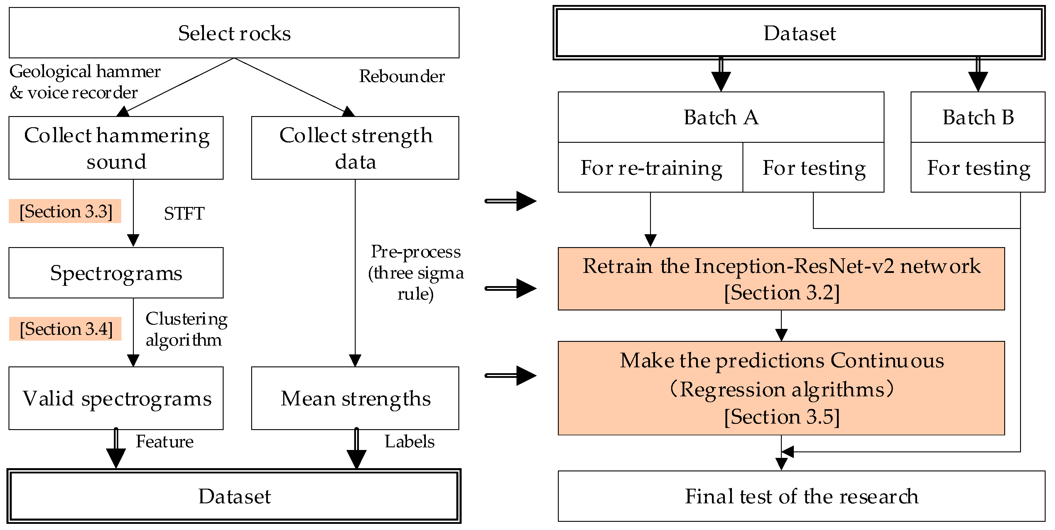
The overall process can be presented as Figure 1. Firstly, several rocks were selected as subjects. For each rock, the strength data was measured with a rebounder and the hammering sound was collected using a geological hammer and a voice recorder. Next, the hammering sounds were transformed into spectrograms, and then the spectrograms were filtered with a clustering algorithm. On the other hand, the measured strength data was pre-processed. After that, some spectrograms and their corresponding strength data (Batch A) were used to retrain the Inception-ResNet-v2 model, and the other spectrograms and their corresponding strength data (Batch B) were used for the final test of the method.

In the next sub-sections, the core technologies of this research are described in details, including the Inception-ResNet-v2 model, the short-time Fourier transformation (STFT), the clustering algorithm, and the regression algorithms.

3.2. Inception-ResNet-v2 Model

Inception-ResNet-v2 was developed from the Inception Net model by Google [28]. Different from Inception v1 to v3, the Inception-ResNet-v2 model takes advantage of the residual networks, successfully improving the accuracy and convergence speed of the original model. In a residual network, as shown in Figure 2, the output of the previous layer is inputted into the middle layer and the next layer together with the output of the middle layer [29]. Therefore, when adjusting the weights using the back propagation method, the gradient from the upper layer can skip over the middle layer up to the lowest layer, ensuring that all the weights can be adjusted effectively. More details of the Inception-ResNet-v2 model can be found in the publications [28,29].

Generally, the fine-tuning process includes four key steps: (1) train a deep learning network based on the source data. In this research, the Inception-ResNet-v2 model has been well-trained. (2) remove the output layer of the network, and reform the size of the output layer according to the target data, (3) initialize the weights of output layer and keep the weights of other layers unchanged, and (4) re-train the network, as illustrated in Figure 3.

3.3. Short-Time Fourier Transformation (STFT) and Spectrogram

In this research, hammering sounds were firstly transformed into spectrograms because of the Inception-ResNet-v2′s strength in image identification. Hence, the STFT was utilized to process the sounds, as follows:

$$S_x\left(n,\omega \right)={\displaystyle \sum _{-\infty }^{\infty }x\left(m\right)}w\left(n-m\right)e^{-j\omega m}$$

(1)

where w(n) represents the window function, and ω is the frequency in radians [30]. In an STFT process, it is important to determine the size of the window. A large window leads to poor time resolution, while a small window leads to a poor frequency resolution. Either window size will degrade the quality of a spectrogram. Moreover, during programming, the sampling frequency fs, the time lapse L, and the frequency discretization N also affect the resolution of the spectrograms. However, it is difficult to determine the exact parameters in different cases. In this research, we found out a set of parameters through repeated experiments to make the spectrograms look clear.

Spectrograms generated by the STFT are presented in Figure 4. In a spectrogram, there are three dimensions that correspond to frequency (vertical axis), time (horizontal axis), and sound pressure (color gradient) or power spectral density (PSD). In the spectrograms example presented in Figure 4, yellow represents high sound pressure, and blue represents low sound pressure. It is easy to distinguish how sound pressures are distributed along with the frequencies in a certain period, how the sound pressures change over time in a certain frequency range, and how the principal frequency changes over time. Specifically, Figure 4a corresponds to the hammering sound of a rock with low strength, Figure 4b corresponds to a rock with moderate strength, and Figure 4c corresponds to a rock with high strength. It is obvious that in Figure 4c the proportion of high frequency is the largest, the attenuating speed is the slowest, and the differentiation of different frequency bands is the clearest.

Additionally, we found that there were no differences in parts of the spectrograms that had frequencies greater than 5 kHz, no matter for high-strength rocks or for low-strength rocks; thus, the parts with high frequency do not contribute to the analysis. Moreover, research has shown that human’s most sensitive sound frequency is 2 kHz–5 kHz [31]. Therefore, only the 0–5 kHz part of the spectrograms was used for identifying strengths.

3.4. Selection of Training Samples Based on Clustering

3.4.1. Script Program for Cutting Hammering Sound

In this study, thousands of hammering sounds were transformed into spectrograms. Therefore, a simple script was programmed to split the hammering sounds automatically. First, for a sound file that contained hundreds of hammering sounds, the time series was iterated to determine a series of mutational points, [t₁, t₂, …, t_n], according to the amplitude, as shown in Figure 5. Next, it was assumed that the hammerings occurred at 10 milliseconds before the mutational points and each hammering sound lasted 150 ms, as shown in the right part of Figure 6. The two durations, 10 milliseconds and 150 ms, were determined by the statistical data in this research. The individual hammering sounds were then extracted, and the STFT was used to transform all the sound fragments into spectrograms.

However, these spectrograms could not be directly used for training because some sound fragments may not contain the right hammering sound. For example, some sound fragments may contain loud talking voices, or some may be produced by hammering at a wrong point by mistake. Therefore, invalid spectrograms should be eliminated to maximize the effectiveness of training.

3.4.2. Binarization and Feature Extraction

For a set of spectrograms that obtained from the same rock, the biggest difference between the valid and invalid spectrograms is the distribution of frequencies. According to this principle, we suggest binarizing the spectrograms firstly to emphasize their features, as shown in Figure 6. The binarization threshold of each spectrogram can be determined using Otsu’s method [32]. Otsu’s method entails dividing an image into two sections (background and object) according to the gray-scale gradient. The formula of Otsu’s method is as follows:

$$g=w_1\times w_2\times {\left({\mu }_1-{\mu }_2\right)}^2$$

(2)

where w₁ is the proportion of the pixels of the object, w₂ is the proportion of the pixels of the background, μ₁ is the mean gray value of the object, and μ₂ is the mean gray value of the background. The optimal gray threshold is determined by finding out the maximum of g.

Following this, each binarization was divided into 10 equal parts along the vertical axis. The number of white pixels in every part was calculated, then normalized by dividing them by the total amount of the white pixels, as shown in Figure 6. In this way, each spectrogram could be represented by 10 features. For example, the spectrogram shown in Figure 6 can be represented by [0.1323, 0.07887, 0.0657, 0.0665, 0.0682, 0.0815, 0.1029, 0.1698, 0.1687].

For a set of spectrograms that obtained from the same rock, the features of the valid spectrograms are similar to each other, while the invalid spectrograms are various. In this study, we assume that the spectrograms can be divided into three categories with a clustering method, and the categories that contain the most spectrograms are regarded as valid spectrograms.

3.4.3. Clustering Based on the Modified K-means Algorithm

The K-means algorithm, as a classical clustering algorithm, is famous for its simplicity and strong clustering ability [33]. As mentioned in Section 3.4.2, we set the value of K as three to divide the binarization spectrograms into three clusters, meaning that there is a major cluster that contained the most binarization spectrograms, and the other two clusters represented two extremes that differed from the major cluster.

However, the K-means algorithm is highly random because the initial seeds are selected randomly, making it easily plunge into local optima. To solve this problem, the initial seed selection is modified. The modified K-means algorithm is as follows:

Algorithm Modified K-means Algorithm

Input: Dataset X = {x1, x2, …, xn}, numbers of clusters N = 3

Output: Clustering result LabelX

1:    For i = 1 to n−1

2:     For j = i to n

3:         Distance(i, j) = the Euclidean distance between xi and xj

4:     End

5:    End

6:    MaxDistance = the maximum of Distance

7:    If number(MaxDistance) > 1

8:       Select one of the MaxDistances randomly and find out its corresponding xmax_i, xmax_j

9:    End

10: Seeds(1) = xmax_i, Seeds(2) = xmax_j, Seeds(3) = Mean(xmax_i, xmax_j)

11: LabelX = Kmeans(X, Seeds)

The modified seed selection method identifies three seeds that have the longest distance from each other, and can ensure that the differences between the three categories are maximized.

The next step is to determine which categories are valid. The category that contains the most spectrograms is regarded as a valid category firstly. By experience, the amount of valid spectrograms occupies approximately more than 85% of the total. Therefore, for the other two categories, if the sum of them is less than 15%, then the spectrograms of the two categories are determined to be invalid; if the sum of them is larger than 15%, then only the smaller category is determined to be invalid.

3.5. Prediction Using Machine Learning

Using the re-trained Inception-ResNet-v2 model to determine the surface strength of rocks is virtually an image classification process. In training the DNN, the inputs are the spectrograms, and the labels are the values of surface strengths. After training, for a new spectrogram, the DNN can give the probabilities that the spectrogram belongs to each of the strengths, and classify it into a class according to the maximum probability, as shown in

Table 1. Prediction result of a spectrogram.

Strength	10	20	30	40	50	60	70	80	90	100
Probability	0.0002	0.0000	0.0098	0.0005	0.0000	0.8806	0.1017	0.0004	0.0006	0.0051

.

It can be seen that the prediction results are discrete. However, surface strength is a continuous variable. To resolve this problem, the probabilities are regarded as the spectrograms’ features extracted by the DNN model. Therefore, every spectrogram has 10 features and one label (strength value). Then, the relationship between the features and the strength values can be fitted with regression algorithms. The regression algorithms used in this research included the K-Nearest Neighbor [34], the Support Vector Machine [35,36], and the Random Forest [37].

4. Experiment and Analysis

4.1. Data Collection

Data for re-training the DNN model comprised the surface strengths and hammering sounds. In this experiment, two batches of data, Batch A and Batch B, were collected, and the rocks in Batch B were different from the rocks in Batch A. Batch A was used for re-training and conducting the preliminary tests. Batch B was used for the final test of the method.

The surface strengths of rocks were measured by an N-type rebound device. An N-type rebound device can measure the rebound values by hitting a rock. As mentioned in Section 2.1, current research has demonstrated that there is a strong link between the rebound value and the UCS. Therefore, in this study, the surface strengths of the rocks were represented by their rebound values.

The objects used in the experiment were rocks that existed in the natural environment. Every rock was intact and at least 0.05 m³ in volume. Rocks were not limited to a particular type. It was not possible to measure the strength of the whole rock mass due to the rock anisotropy, and what was measured was just the strength of one point on the rock. To avoid damage to the surface of the rock caused by measuring one point too many times (especially when the rock was weak), three measuring points close to each other were set on one rock. Each point was hit five times by the rebound hammer. In total, there were 15 rebound values for each rock. Then, the surface strength of a rock could be calculated by filtering the values with the three sigma rule and calculating the mean of the remaining rebound values. Moreover, before measuring, the weathered layers of the rocks were removed.

Table 2. Rebound values of A and B.

No.	Mean	Variance	No.	Mean	Variance	No.	Mean	Variance
A1	20	1.12	A6	54	1.56	B1	61	1.88
A2	73	1.13	A7	67	1.18	B2	48	2.37
A3	48	1.50	A8	58	1.72	B3	64	2.39
A4	39	1.73	A9	26	1.00	B4	72	2.43
A5	62	1.15	A10	44	1.88	B5	66	1.92

shows the measurements of 15 rock samples A1–A10 (strengths of Batch A) and B1–B5 (strengths of Batch B). In addition, the rocks included granites, basalts, killas, and andesites. However, the types and mineral compositions of rocks were not regarded as the influential factors.

The reason why we divided the whole dataset into two batches was that an algorithm (even DNN) may be sensitive to the data that similar to the training data. The rocks in Batch B were different from the rocks in Batch A, and the strengths of Batch-B rocks were also different from the Batch-A rocks. A part of Batch A was for the primary test of our method, and the whole data of Batch B was for the further verification of the generalization of the method.

After measuring the strengths, each rock was hammered 200–260 times with a geological hammer around the three measuring points. A voice recorder was used to record the hammering sounds. The hammering rate was approximately one-two times per second, and the hammering force was slightly varied every 20–30 times to ensure the variability of the hammering force. The voice recorder had two channels, and its sampling frequency was 24 kHz.

It should be noted that in fact the hammering force mainly affects the amplitude of the hammering sound (sound level). Therefore, we did not hammer the rocks too hard, but put the voice recorder very near the hammering points to obtain clear sounds, and in this way prevented (or reduced) damage of the rock surface. Despite that, some rocks were still damaged in our experiment, and in these cases, new hammering points near the old ones were selected to continue the experiment. However, for those rocks of which nearby areas of the measuring points were all damaged, the measuring processes were terminated immediately.

4.2. Producing Spectrograms

With the script described in Section 3.4.1, 2410 hammering sounds were extracted from the sound files. The parameters used in STFT were as follows: the size of the window function R = 64, the time lapse L = 32, the sampling frequency fs = 24 kHz, and the frequency discretization N = 8192.

As shown in Table 2, there are 10 different rebound values in total, each of which corresponded to 200–260 spectrograms. According to the rebound values, all the spectrograms of Batch A were assigned to 10 different file folders, and the folders were named by their rebound values. After that, the modified K-means clustering algorithm described in Section 3.4.3 was used to remove the invalid spectrograms in every folder.

Table 3. Clustering results of spectrograms.

No.	Total	Cluster 1	Cluster 2	Cluster 3	Removed	Remained
1	201	24	52	125	Cluster 1	177
2	217	85	103	29	Cluster 3	188
3	258	73	16	169	Cluster 2	242
4	239	136	67	36	-	239
5	260	96	18	146	Cluster 2	242
6	232	105	99	28	Cluster 3	204
7	252	10	81	161	Cluster 1	242
8	253	139	20	94	Cluster 2	233
9	259	154	90	15	Cluster 3	250
10	239	2	74	163	Cluster 1	237
Total	2410	-	-	-	-	2254

shows the filtering result of Batch A.

4.3. Re-Training the DNN

In Batch A, there were 2254 spectrograms. Figure 7 shows some of the spectrograms with different strengths.

These spectrograms were then used to re-train the Inception-ResNet-v2 model. The parameters set for training comprised an initial learning rate of 0.002, a learning rate decay of 0.7, an epoch number of 100, and a batch size of 10. About 80% of the data were used to train the network, and the remaining 20% were used for validation. The evaluation indicators included the accuracy and the loss. After training, the structure and weights of the network were determined and were not changed any further. The training process is illustrated in Figure 8.

As presented in Figure 8, in the first 1500 iterations, the accuracy grew rapidly. After about 5000 iterations, the accuracy reached 0.9, and then grew slowly. At the end of the training, the accuracy was 0.945. In the first 3000 iterations, the loss dropped quickly, then held steady between 0.50 and 1.00. We stopped the training at the 18000th step, because the loss showed that it would not be further decreased, and more training would lead to an over-fitting.

4.4. Predicting Rock Surface Strength

The training results demonstrate that the fine-tuned DNN can classify the spectrograms with high accuracy. In the next step, the outputs of the network were regarded as the features of the spectrograms. Three regression algorithms, including the KNN, the SVM, and the RF, were then tried to fit the relationship between the features and the strengths.

4.4.1. Predictions of Batch A

First, Batch A was used as the input to test the method. The regression algorithms were used as follow: (1) in the SVM, the Gaussian kernel function was adopted; (2) in the KNN, the number of N was set to 20; (3) in the RF, the number of trees was 800, and the maximum depth was nine. Figure 9 displays the regression results.

The R² is used to measure the goodness of fit (GOF). Figure 9a,c, and e show that all the three algorithms can reach a high R² of more than 0.95. The R² of the KNN algorithm is the largest and is more than 0.98. The norm of residual is another measure of GOF, and a lower norm signifies a better fit. Among the three algorithms, KNN has the smallest norm of residual. Figure 9b,d,f are the distributions of the errors of the three algorithms. It also indicates that KNN is more accurate than the other two algorithms: the range of the errors is within [−20, 20], the errors that larger than −2.5 and smaller than 2.5 occupy 96.88%, and the errors in the range of [−5, 5] occupy 97.86%. Comprehensively, KNN gets the best performance, and the followings are the SVM and the RF.

4.4.2. Predictions of Batch B

The samples in Batch B had neither participated in the deep network re-training nor the regression process. Moreover, four out of five of the labels (rebound values) of Batch B were out of the range of Batch A. The configurations of the regression algorithms were the same as that in Section 4.4.1.

Table 4. Regression results of Batch B.

Strength	Mean Errors			Variance
	KNN	SVM	RF	KNN	SVM	RF
48.00	−1.75	−1.11	−1.96	2.19	1.23	2.33
61.00	1.68	1.17	1.49	2.14	2.31	2.41
64.00	−1.75	−0.58	−1.79	6.30	4.66	5.60
66.00	2.44	1.62	1.18	3.15	1.81	3.29
72.00	5.19	6.95	5.73	5.65	4.34	6.47

shows the mean errors and variances between the predictions and the real strength values.

As presented in Table 4, the predictions of the SVM have the minimum mean errors except for the fourth and the fifth sample sets, and have the minimum variance except for the second set. The minimum mean error of the 5th samples sets is predicted by KNN. The minimum variance of the second set is also predicted by KNN. Overall, SVM predictions are the best, the following is KNN, then RF.

4.5. Discussion

Based on the results presented in Section 4.4, it can be seen that the predictions of Batch A are significantly better than the predictions of Batch B. For one thing, the data of Batch A and Batch B were collected by two groups of researchers, and there might be some non-standard operations when collecting Batch B—for example, the hitting directions and the hitting speeds when using the rebound device. Further, the re-trained deep learning network was used for image classification, and there were only 10 clusters in the training sample. By enlarging the size of training data, the prediction of Batch B can be improved. For Batch A, the KNN algorithm made the best predictions, meaning that the fitting accuracy of KNN was the highest. For Batch B, the SVM achieved the best results, meaning that it had the strongest generalization ability in this regression.

5. Conclusions

In this paper, a new non-destructive measuring method for rock surface strength is presented based on the DNN technique and spectrogram analysis. The process comprises four steps: (1) collect hammering sounds and strength data, (2) produce spectrograms of the hammering sounds and remove invalid spectrograms using a modified K-means algorithm, (3) re-train the Inception-ResNet-v2 model by taking the spectrograms and strength data as the inputs and labels respectively, and (4) use regression algorithms to make the prediction results continuous. The validation shows that the strengths (represented by rebound values) of almost all the samples can be predicted within an error of [−5, 5].

Moreover, the combination of the re-trained DNN and KNN has the highest fitting accuracy, and the combination of the re-trained DNN and SVM has the strongest generalization ability. Therefore, if the size and the number of clusters of training samples are large, we recommend KNN for regression. Otherwise, SVM is recommended.

The proposed method was accomplished using Python and Tensorflow programming; however, it should be noted that the contribution of this research is not about a new deep neural network, and both the Inception-ResNet-v2 model and transfer learning are well-established techniques. This research is an application of them, and is aimed at presenting an effective and simple method for field survey. Overall, the proposed method offers great potential in supporting the implementation for efficient rock strength measurement methods in the field.

A noted limitation of this research is related to the use of a rebound device to capture the raw rock strength data, under experimental conditions. The precision of the rebound method is low, and the measurement is easily affected by hitting directions and hitting speed. In the subsequent work, higher precision techniques, such as acoustic emission techniques, will be considered to optimize the performance of the method further.