An Intelligent Milling Tool Wear Monitoring Methodology Based on Convolutional Neural Network with Derived Wavelet Frames Coefficient


1
School of Aerospace Engineering, Xiamen University, Xiamen 361005, China
2
New Jersey Institute of Technology, University Heights Newark, NJ 07102, USA
*
Author to whom correspondence should be addressed.
Appl. Sci. 2019, 9(18), 3912; https://doi.org/10.3390/app9183912
Submission received: 24 July 2019
/
Revised: 5 September 2019
/
Accepted: 10 September 2019
/
Published: 18 September 2019
(This article belongs to the Special Issue Machine Fault Diagnostics and Prognostics)
Abstract
:Tool wear and breakage are inevitable due to the severe stress and high temperature in the cutting zone. A highly reliable tool condition monitoring system is necessary to increase productivity and quality, reduce tool costs and equipment downtime. Although many studies have been conducted, most of them focused on single-step process or continuous cutting. In this paper, a high robust milling tool wear monitoring methodology based on 2-D convolutional neural network (CNN) and derived wavelet frames (DWFs) is presented. The frequency band of high signal-to-noise ratio is extracted via derived wavelet frames, and the spectrum is further folded into a 2-D matrix to train 2-D CNN. The feature extraction ability of the 2-D CNN is fully utilized, bypassing the complex and low-portability feature engineering. The full life test of the end mill was carried out with S45C steel work piece and multiple sets of cutting conditions. The recognition accuracy of the proposed methodology reaches 98.5%, and the performance of 1-D CNN as well as the beneficial effects of the DWFs are verified.
1. Introduction
In the past few decades, equipment-manufacturing technology has developed rapidly. The automation level and production capacity of the machine tool are significantly improved. However, there are still many uncertain factors in the production process, such as tool wear and breakage, which are an important and common source of machining problems. Tools are end-effectors that execute efficiency and quality, and are the cost-intensive consumable parts [1]. The tool condition monitoring system can achieve immediate benefits, and thus receive extensively study [2]. The industrial manufacturing processes are dynamic and complex, especially for multi-axis computer numerical control (CNC) equipment, tools often perform a variety of tasks. Work piece properties such as hardness and cutting allowance also change frequently, which makes the condition of the tool difficult to predict. According to statistical research, one effective tool condition monitoring system can help to increase the cutting speed, maximize the effective working life of the tool and reduce machine tool downtime by pre-arranging tool change time [3].
Severe damage such as breaks or large-size chippings can be reliably identified online because the signal patterns of these phenomena are rarely obvious [4]. Tool failure due to the accumulation of wear and weak chipping is relatively difficult to detect in time. At present, there have been many successes in tool wear monitoring during continuous cutting [5,6,7]. However, it still requires more effort in milling, where tools and material removal processes are more complex. A tool condition monitoring system can be divided into three parts: Sensing and data acquisition, data processing and feature engineering, and pattern recognition and classification [8].
Sensing and data acquisition methods include direct acquisition and indirect acquisition. The contact detection is the most widely used direct approach, but the tool can only be measured after the end of one process. The indirect method that detecting the tool health condition by physical signals is more suitable for online measurement. The cutting force is the most mature indirect measurement method [9]. Nouri M. established a milling force model and then coupled the normalized tangential and radial forces in the model into a single parameter to monitor the wear of the end mill [10]. Liu C. combines cutting force signals and vibration signals to identify tool wear and work piece deformation during processing of thin-walled parts [11]. Jose B. adopts the cutting force to monitor tool wear and product surface quality during the CNC turning of D2 steel [12]. Nevertheless, the dynamometer is costly and does not fit large work pieces such as engine cases. Acoustic emission sensor [13], current/power sensor [14] and sound pressure sensor [15] also have their own advantages and disadvantages. In contrast, vibration acceleration sensing technology offers comprehensive advantages in terms of cost, flexibility, non-intrusiveness, information capacity and industrial reliability. Nakandhrakumar R. applied torsional–axial vibrations to monitor flank wear during drilling, with an accuracy of 80% [16]. Mohanraj T. extracted the effective features for tool condition from the vibration signal under the interference of the cutting fluid [17]. The ever-increasing theoretical knowledge of sensing and signal processing can further enhance the reliability and signal-to-noise ratio of vibration sensors. Yan R. proposed a closed loop calibration system to improve the calibration accuracy and efficiency of vibration sensors [18].
Signal processing and feature engineering aims to clean the raw data, segment and label the valid data, and further extract feature vectors to suit the needs of the decision subsystem. As a complex process system, no matter what kind of sensing method is used, we collect a mixture of various signals and noise. For the vibration signal, the unbalance of rotating parts, the inertial impact of reciprocating parts, and the insufficient smoothness of each shaft will produce forced vibration. Du Z. used an adaptive variable window to locate the signature segments in the signal and successfully align them [19]. Chudzikiewicz A. proposed a modified Karhunen–Loève transformation algorithm for preprocessing acceleration signals [8]. For the original time domain signal, principal component analysis can be used to extract the effective features [20]. The regularization based on convex sparsity can be used to decompose noisy signals, while non-convex regularization can further promote the sparsity of reconstructed signals, while preserving the global convexity [21]. Studies have also shown that the method of extracting features from frequency domain signals is easier to implement and more stable [22]. The monitoring signals in the milling process are often similar to the modulated signals, and the information carried in different frequency bands is quite different. Therefore, the time–frequency domain analysis represented by wavelet transform becomes a powerful tool. Segreto T. used the wavelet packet transform to extract the feature vector from the tool-holder vibration signal to identify the machinability of the nickel–titanium alloy turning process, and the recognition accuracy is not less than 80% [23]. Madhusudana C. employed dual-tree complex wavelets to extract features from sound pressure signals to monitor the health of indexable inserts [15]. He W. proposed a sparsity-based feature extraction method using the tunable Q-factor wavelet transform with dual Q-factors [24]. Kurek J. adopted wavelet transform to decompose the original monitoring signals, and extract features from each sub-signal to form a mixed feature vector. The trained RF model identifies the wear state of the drill with an accuracy of no less than 96% [25]. Hong Y. applied the wavelet packet decomposition to the low SNR cutting force signal in the micro end milling process, which effectively improved the feature extraction efficiency [26].
The decision subsystem is the most important part of achieving tool condition monitoring. It is a complex nonlinear model that identifies the health condition of the tool based on the feature vector. Various machine learning models have succeeded in the field, such as artificial neural network (ANN) [27], fuzzy inference systems (FIS) [28], hidden Markov model (HMM) [29] and support vector machine (SVM) [30] and others [31,32,33]. The special network structure makes the machine learning model also able to achieve ideal classification accuracy when the data set is small, but they are not suitable for data samples with big size. This imposes stringent requirements on feature engineering. In addition to the evolutionary factors we expect to monitor, other operational parameters of the monitored object will also affect the features extracted by the feature engineering. [8]. For the milling process, not only tool wear, but also cutting condition adjustment and changes in work piece material properties have significant effects on statistical features such as RMS, kurtosis and entropy. The portability of the system is thus reduced and is not suitable for automated production sites where cutting conditions are variable.
The new learning algorithms empower us to build neural networks with more layers, as well as train them with big samples. Coupled with the extremely increasing computing power, especially parallel computing, the powerful feature extraction capabilities of convolutional neural network (CNN) have been validated in many pattern recognition [34,35] and phonetic recognition projects [36,37]. The monitoring signal such as vibration acceleration is similar to the speech signal, and the line graph or time spectrum of the signal is similar to the visual image. Therefore, many scholars adopt the CNN to equipment fault diagnosis and health monitoring. Sun W. adopts CNN to the identification of gear faults, and the recognition rate reached 99.97% under the enhancement of double-tree complex wavelet [38]. Wang F. proposed an adaptive convolutional neural network for fault diagnosis of rolling element bearings, which proved to be superior to ANN and SVM [39]. Chen L. mapped the original monitoring signals into feature maps to fit the 2-D convolutional neural network, and the recognition accuracy of bearing faults was not less than 90% [40]. Yang F. mapped the raw 1-D signals into 2-D images to identify the vibration state of the machine tool. The recognition accuracy of the 2-D CNN is not less than 90%, which is obviously superior to the traditional signal-feature-model [41].
This paper proposes a tool condition monitoring system based on 2-D convolutional neural network and assisted by complex wavelet. The reminder of this paper is organized as follows. In Section 2, some background and preliminaries are reviewed. In Section 3, we detailed the proposed monitoring system, including data acquisition, data preprocessing and methods for constructing 2-D maps. The spectrum band of the spindle vibration signal is converted to a normalized data map to train the convolutional neural network. In Section 4, based on the collected data sets, we optimized the hyperparameters of CNN through a series of single factor experiments. In Section 5, the parameter-optimized monitoring system is implemented in the multi-parameter cutting experiment to monitor the wear state of the tool, and the monitoring effect is compared with other methods. Section 6 finally presents our conclusions.
2. Background and Preliminaries
2.1. Translation-Invariant Signal Decomposition Using the Derived Wavelet Frames
Transient features are important for identifying dynamic changes in tool wear and breakage. However, irrelevant low frequency vibrations and background noise often overwhelm them [42]. Fidelity signal decomposition is beneficial for improving the signal-to-noise ratio and reducing the subsequent computation of the model. Due to the lack of shift-invariance, the ability of traditional wavelet transform to mine repetitive shock vibrations in the raw signal is relatively weak [43]. In this section, we introduced derived wavelet frames to perform a nearly shift-invariant multiresolution analysis. Derived wavelet frames (DWFs) are based on dyadic doubletree complex wavelet packets and are supplemented by non-dyadic implicit wavelet packets. The latter enhances the ability of the algorithm to extract transition-band features.
2.1.1. Dual-Tree Complex Wavelet Packet Decomposition
Dual-tree complex wavelet packet decomposition (DCWPD) is constructed based on dual-tree complex wavelet basis, which it consists of two scaling functions and two wavelet functions.
In orthonormal cases, for the complex valued wavelet function:
there is a restriction of approximate Hilbert transform shown as:
where and are the real part and imaginary part of respectively, and is the imaginary unit. Equivalently, a half sample delay equation exists for impulse response functions of imaginary wavelets and real wavelets .
Let the transform of a discrete series be represented as:
The filter-bank structure of DCWPD is shown in Figure 1.
The notation denotes or . This means that the real filter tree of DCWPD is independent of the imaginary filter tree, but uses the same filter structure. Both are iterative decomposition processes based on a special hybrid wavelet bases and a binary tree structure. More details about the two filter branches can be found in the original article published by Kingsbury and Selesnick [44]. The employed filters can be classified into three categories:
- (1)
- Wavelet basis at the first level. These filters are (Figure 2a,b)), and they satisfy the following equation.
- (2)
- Conventional dual-tree complex wavelet basis to obtain wavelet series . The associated filters are (Figure 2c,d).
- (3)
- Additional basis to generate extended wavelet packet series . The associated filters are:
2.1.2. Implicit Wavelet Packets and the Frequency-Scale Paving of Derived Wavelet Frames
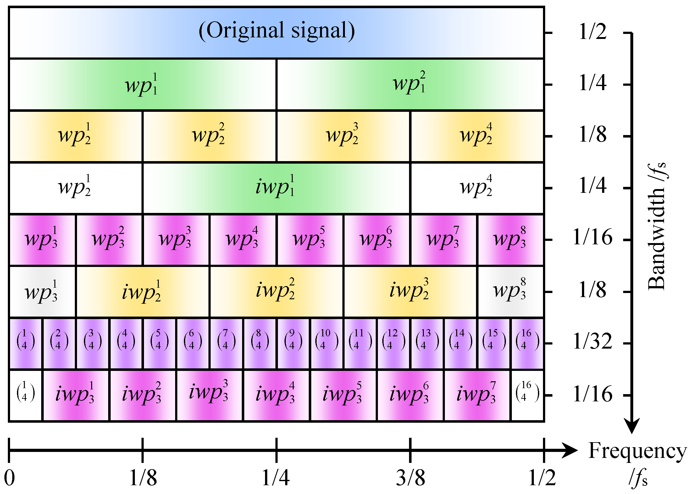
The frequency response curves of the dyadic wavelets overlap each other at the boundary, so that the performance of extracting incipient vibration signatures located in transition bands is not perfect. In order to improve its performance supplementary, implicit wavelet packets were constructed based on DCWPD. The derivation process of the implicit wavelet packets (IWPs) mainly includes the following steps, wherein denotes the input signal.
Step (1): Decompose the original signal into a set of sub-signals at multiple scales based on the dual tree wavelet packet decomposition: .
Step (2): Reorganize set according to the order of central frequency, and generate a new sequence of sub signal :
The conversion relationship of the sequence number of a sub-signal in these two sets is:
For , let the binary code of the index be:
A new integer is expressed as:
where is defined as:
Step (3): Generate the implicit wavelet packet:
The frequency-scale paving of implicit wavelet packets are represented by the block identified as in Figure 3. It can be seen that implicit wavelet packets realize multiresolution analysis around fixed central frequencies. Mathematical definitions of such sets can be expressed as:
2.2. The Feature Learning Process of CNN
As a deep learning model, CNN can adaptively extract implicit features from input data, and has achieved many successful applications on multi-classification issues. Convolution and down sampling operations enable CNN to simplistically stack deep learning networks without computational explosions, taking into account learning accuracy and learning efficiency. As shown in Figure 4, the 2-D convolutional neural network includes an input layer, an output layer and a series of hidden layers. In the hidden layer, the input image is first convoluted with the filter to extract features, which are then down sampled to obtain a feature map that is halved or smaller in size. There are several published methods to convert a temporal signal into a 2-D matrix to train 2-D CNN [38,47]. In this paper, a segment of the spectrum of raw signal was converted to logarithmic coordinates and normalized, and finally folded into a 2-D matrix as the input of the 2-D CNN. The feature map will continue to transmit information in the network as input to the next hidden layer.
2.2.1. Convolution Layer
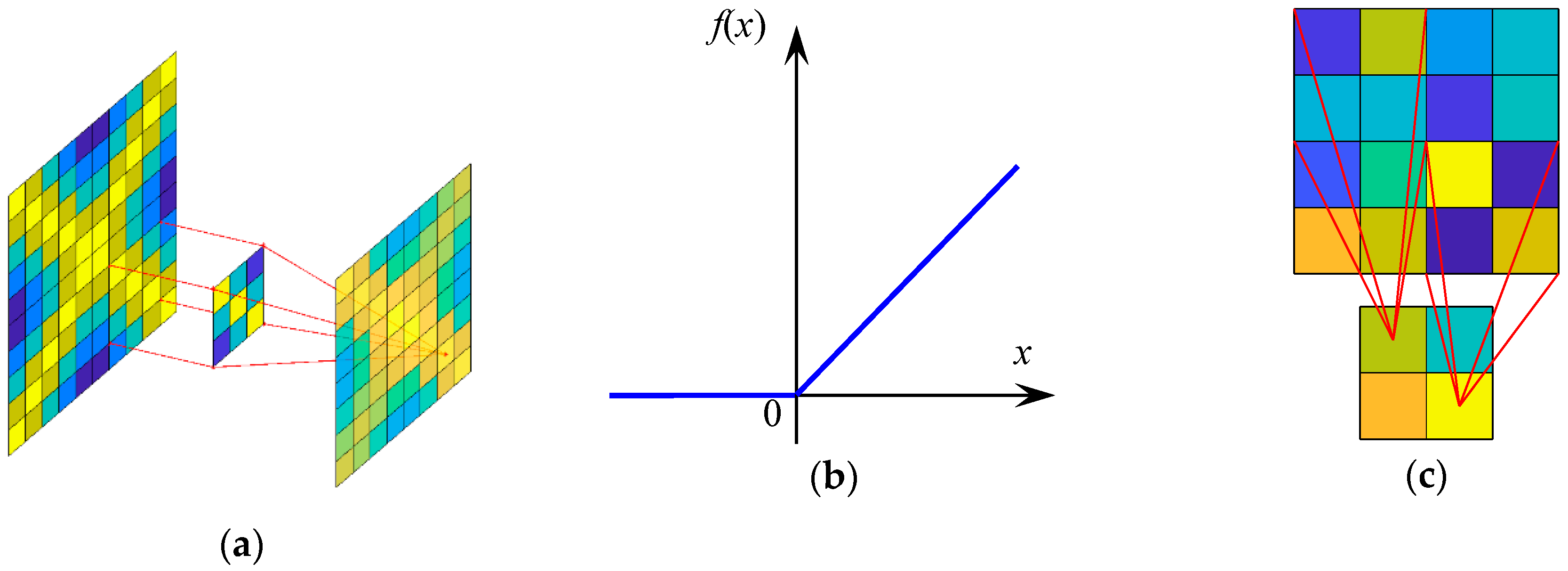
In the convolutional neural network, the convolution layer, the activation layer and the pooling layer are fixedly combined to form a nonlinear hidden layer. As shown in Figure 5a, the 2-D convolution kernel characterizes the local texture for the image, and the 1-D convolution kernel characterizes the tone for the sound signal. In the case of success, the width of the neural network model, that is, the number of convolution kernels of each convolution layer, is generally set according to the specific conditions of the identification task. The size of the convolution kernel is generally small, and the entire image shares the same weights. This reduces the computational complexity and gives the model translation invariance.
The convolution process of obtaining the j-th feature map in the l-th convolution layer can be expressed as follows:
where denotes the i-th feature map generated from l-1th pooling layer ; denotes the weight matrix of the j-th filter in the l-th convolution layer; denotes the j-th element of the bias of the l-th convolution layer; denotes the subset associated with in the set of feature maps output from the l-1th pooling layer and ‘’ denotes the 2-D convolution operation. The activation function is the core of machine learning, which turns the model into a nonlinear model to enhance the expressive power of the model. In this paper, the rectified linear unit (ReLU) is employed, which is defined as follows:
As shown in Figure 5b, the output gradient is always 1 on the positive half-axis, so the model can converge quickly. However, the negative half-axis output is always zero, which endows the model with good sparsity. Recent research cases have shown that the ReLU can effectively solve the gradient diffusion problem and show better generalization capacity than the saturating nonlinearities such as the sigmoid and tangh functions with respect to large scale training datasets [48].
2.2.2. Pooling Layer
The pooling layer immediately follows the activation layer, and it has two main functions: First, spatially down sampling the image to reduce the size of the feature map as well as keep the number of features in a reasonable range as the number of feature maps increase. Second, the filter of the subsequent convolution layer obtains a larger receptive field and can extract features of a larger size. Average-pooling and max-pooling are two of the most common pooling methods across various tasks. In this research, max-pooling is chosen for the pooling layers, as it is reported particularly suitable for the separation of features that are very sparse [49]. As shown in Figure 5c, the pooling layer can be defined as follows:
where denotes the j-th feature map in the l-th pooling layer; denotes the j-th feature map generated from l-th convolution layer; denotes the j-th scaling factor of the l-th pooling layer, denotes the j-th bias of the l-th pooling layer and represents the subsampling function.
2.2.3. Fully Connected Layer
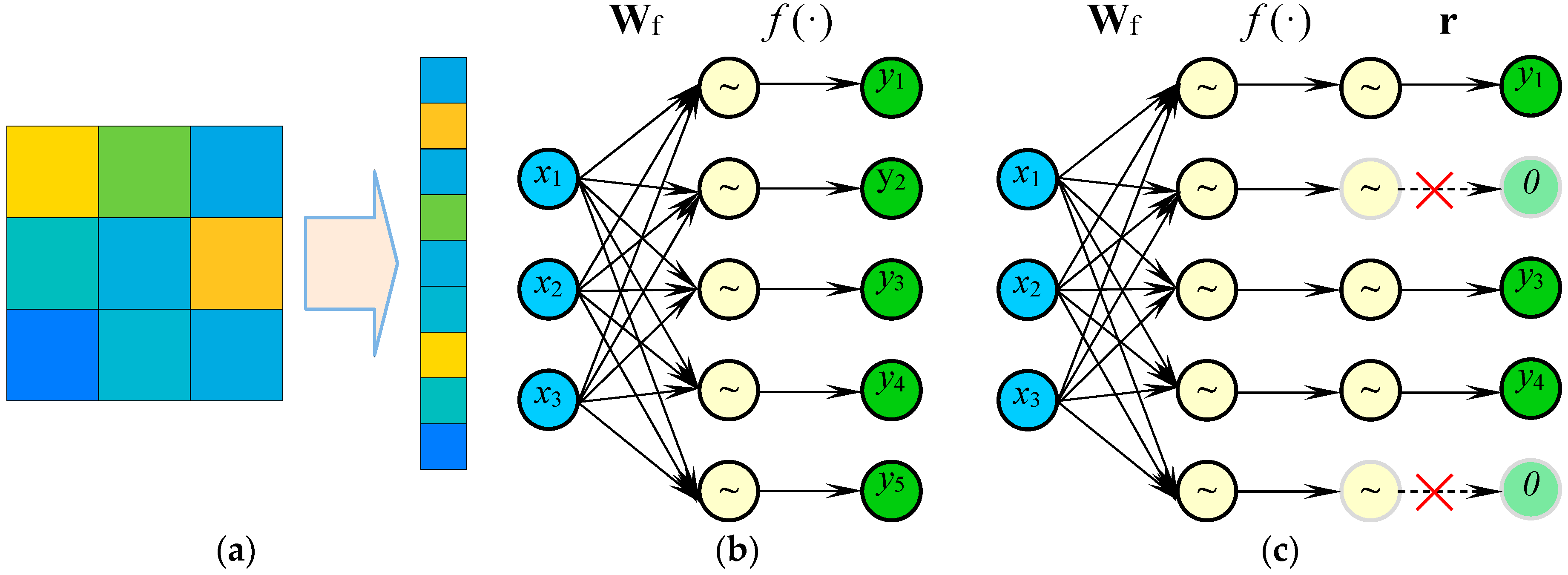
The feature maps convert into a 1-D feature vector through a flatten layer, as shown in Figure 6a. Next is a set of fully connected layers, as shown in Figure 6b, to implement classification or regression. Adding a dropout layer in the middle of the fully connected layer has proven to be an effective way to reduce overfitting since it can prevent the network from becoming too dependent on any small combination of neurons [50]. A fully connected layer enhanced with Dropout is shown in Figure 6c, the output can be represented as the following:
where denotes the input feature vector; is the weight matrix and is a binary vector of size whose elements are drawn from a Bernoulli distribution with parameter , where denotes the dropout rate.
Based on local perception and weight sharing, convolutional neural networks maximize the reference of sample local information to classification. As the tool wears, the contact state of the tool with the work piece changes. The time domain signal and the spectrum shape will change accordingly. This is similar to speech recognition and image recognition. It can be inferred that the convolutional neural network can effectively classify the vibration signals of the tool in different wear states.
3. Proposed CNN + DWFs Methodology and Dataset
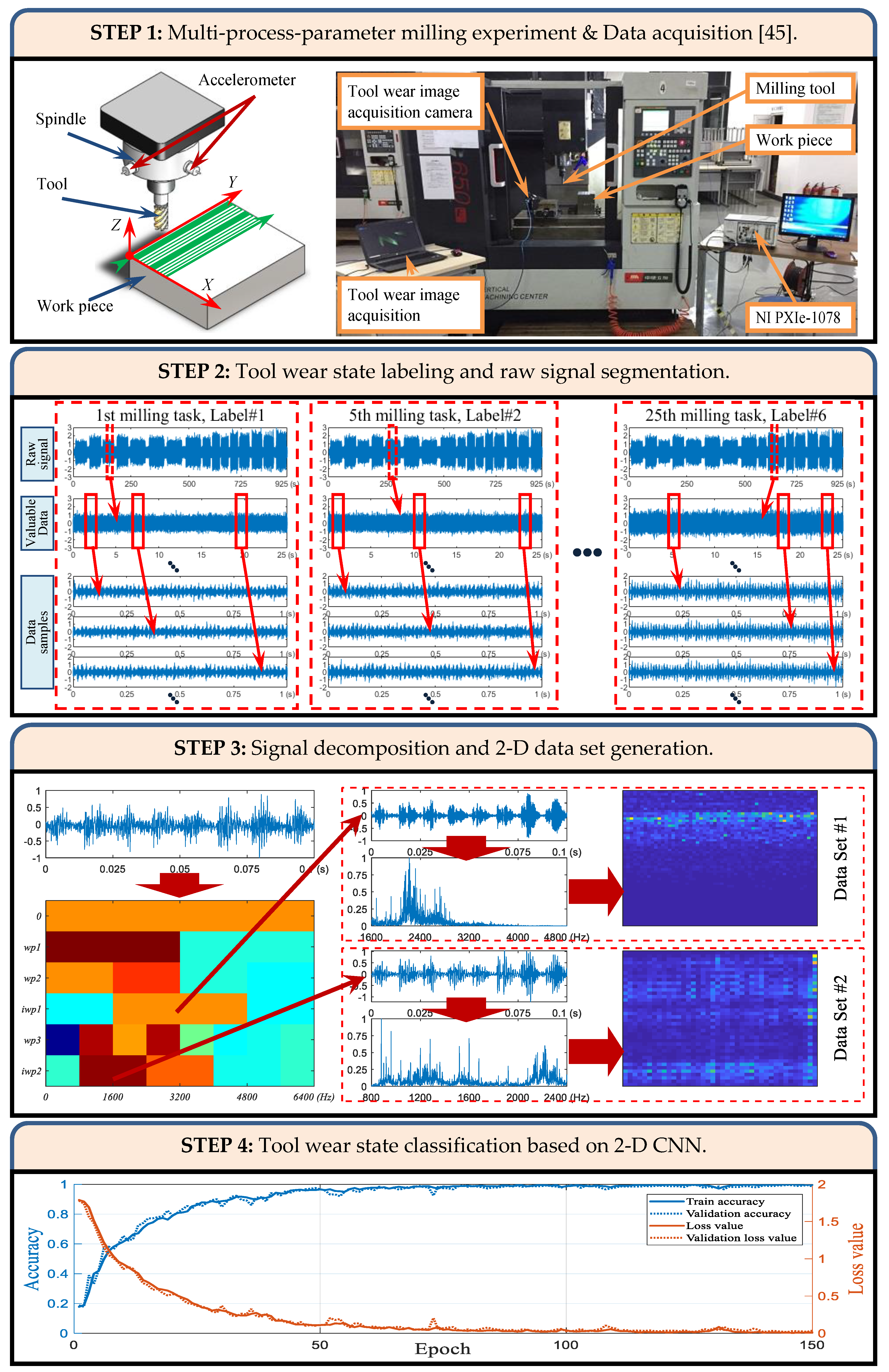
In this section, an intelligent recognition method for tool wear state based on convolutional neural network enhanced by derived wavelet frames was proposed. The proposed method was composed of four major steps, as illustrated in Figure 7.
3.1. Multi-Process Parameter Milling Experiment and Data Acquisition
In order to verify the effectiveness of the proposed method, a series of S45C steel plane milling experiments were conducted on VMC650E/850E machining center (Shenyang Machine Tool Company (Shenyang, China)), as shown in Figure 7. The work piece was an S45C quenched and tempered steel solid block of size . Uncoated four-fluted carbide end mill in diameter was used to perform the cutting experiment. The overhang was set to while the overall length was . Two accelerometers mounted on the spindle housing, parallel to the X-axes and Y-axes. The raw vibration signal was collected via the NI PXIe-1078 data acquisition platform, and the sampling frequency was 12.8 kHz.
At the industrial manufacturing site, the machine tool will adopt different cutting conditions according to the characteristics of the product. In order to better simulate the actual production, four different combinations of cutting conditions were used in the experiment, as shown in Table 1. Milling along the Y-axis of the machine tool, the four combinations of cutting conditions are executed in sequence, and four milling passes are performed under each combination of cutting conditions. Each sixteen milling passes forms a milling task that simulates the manufacturing of a product. Each time a milling task is completed, the machine is paused and images of the cutting edges of the tool are acquired.
3.2. Tool Wear State Labeling and Raw Signal Segmentation
In the International standard ISO 8668-2, regarding the tool-life criteria, the first recommendation is the width of the flank wear land (VB). Nevertheless, due to the lack of necessary measurement equipment, the author failed to obtain this data during the experiment. On the other hand, as the cutting time increases, the tool will inevitably wear out gradually. A total of 25 milling tasks were performed in the experiment. The authors therefore chose six out of the 25 milling tasks at the same interval (the first, fifth, tenth, fifteenth, twentieth and twenty-fifth) and defined that the tool was in different wear states during the six milling tasks. Then, the raw monitoring data of the six milling tasks were libeled as respectively.
The spindle-vibration-acceleration signal for each cutting task is completely collected, with the data of the cutting period being approximately 12 min. The vibration during the idle period is significantly weaker than the cutting period, and there are significant differences in the spectrum. In this paper, the turning point of the effective value of the signal is adopted in order to determine the intersection time of the idle and the milling, and then partition the data of the idle period and the milling passes. According to experience, cutting conditions such as spindle speed and feed rate can decisively affect the cutting process and even obscure the loss of sharpness. Due to different feed rates, the cutting time for each milling pass is not the same. The 9th to 12th steps are the shortest, 120 s; the 5th to 8th steps are the longest, 240 s. For each milling pass, 50 data segments of 1-s duration are extracted from a random initial time in the valuable data of each milling pass. Thus, there are 800 raw signal samples for each cutting state, and the total capacity of the raw signal data set is 4800.
It should be noted that in this paper, the signal segments in the same milling task are set to the same label. That is, the cutting conditions of the signal samples in the data set are unknown.
3.3. Signal Decomposition and 2-D Data Set Generation
During the milling process, the impact of the cutting edge on the work piece is one of the main excitations of the spindle. As a complex mechanical system, the machine tool spindle’s response to the cutting impact is complex and interfered by other excitations such as shaft eccentricity and mesh impact. The acquired vibration signal is a complex mixture, including harmonics of excitation frequencies, resonance of mechanical parts and broadband Gaussian noise. Although, the ability of deep neural networks to extract implicit features from input has been widely recognized. Using advanced signal processing knowledge to extract the informative sub-signal from the raw signal is undoubtedly beneficial for CNN to further extract effective features. Drawing on the experience of feature engineering in traditional fault diagnosis, the information of transient impact in vibration signals is often concentrated in certain frequency bands.
Kurtosis is often used to select the proper demodulation band for further data processing and feature extraction since it can measure the impulsiveness of the signal [51,52]. Figure 8 shows the normalized mean kurtosis map of 20 samples for each subset. The raw data samples were decomposed using the DWFs, the number of decomposition layers is set to 3. A subset of 20 samples was randomly selected for each set of cutting conditions for each tool wear state. It can be seen that the kurtosis of the reconstructed signals in different frequency bands was quite different. At the same time, for every subset, the kurtosis of the frequency band and were higher than other frequency bands of the same layer. A wider frequency band may contain more feature information, but it also increases the computational complexity of the neural network. Therefore, and were utilized to create data sets in 1-D format, respectively. Compared to 1-D convolution, 2-D convolution creates a broader connection between the elements in the inputs. This means that for a particular frequency, 2-D CNN can learn more about its relationship to other frequencies. For the advantages of 2-D convolution, this paper folds the 1-D band spectrum into a 2-D matrix to create a 2-D data set.
Transforming the temporal signal into the frequency domain and training the neural network with the spectral samples could eliminate the interference of the initial phase and reduce the difficulty of recognition. On the other hand, the length of the temporal signal sample was 12800 data points (1 s). Cutting the spectrum of the uninformative band would significantly reduce the size of the sample, further significantly reducing the computational time of the CNN.
The spectral samples were then converted to logarithmic coordinates and normalized. The final step was to fold the sample into a 2-D matrix to accommodate the 2-D CNN format requirements for the input.
3.4. Tool Wear State Classification Based on CNN
The data set was randomly divided into three subsets, named as the train set, validation set and test set. The CNN network was trained with the train set and validation set. After the training process was completed, the test set that did not involve the training process was used for the test.
In this paper, data processing, CNN training and tool wear state recognition were all implemented on a single PC. The processor model was Intel Core i7, the CPU memory capacity was 8GB and the GPU memory capacity was 4 GB.
4. Parameter Optimization for CNN
4.1. CNN Structure Optimization
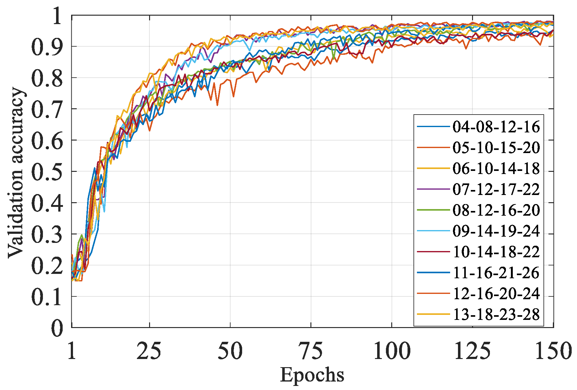
The modeling capabilities of convolutional neural networks depend on the effects of their depth and width. In theory, any non-linear data distribution can be fitted as long as the model is deep enough and wide enough. However, for a simpler classification problem, blindly expanding the network model will not only cause a surge in feature mapping, but also lead to serious over-fitting. In order to optimize the width of the model, 10 neural network models with different widths were constructed. The 10 models have the same structural form, consisting of four convolution layers immediately followed by pooling layer and two fully connected layers. However, the widths of the respective convolution layers were different, and the number of filters in each convolution layer was as shown in Figure 9. In the legend, ‘04-08-12-16’ indicates that the number of filters in the four convolution layers was 4, 8, 12 and 16, respectively.
In this study, we used the cross entropy as the loss function, and adapted the Adam optimizer. Cross entropy is an efficient objective function for combinatorial and continuous optimization and is now widely used to train neural networks for classification [53,54]. Experimental studies have shown that the cross entropy loss function has significant, practical advantages over squared-error [55]. A series of advantages of the Adam optimization algorithm have been widely recognized, such as straightforward to implement, high computationally efficiency, low memory space requirements and invariant to diagonal rescaling of the gradients. Moreover, the adaptability of Adam optimizer is powerful, and there is typically little requirement to hyperparameters tuning [56].
A ten-fold crossover experiment was performed using 2-D dataset #1 with a fixed 150 epoch. Figure 9 shows the validation accuracy convergence graph for each model’s typical training process. Figure 10 shows the average test accuracy and average time consumption per epoch for each model’s ten-fold crossover experiment. It can be seen from Figure 9 that as the width increased, the learning speed and convergence stability of the model increased. At the same time, however, the computational complexity of the model also rose rapidly. It can be seen from Figure 10 that the duration of the single-epoch training was increasing. Considering the modeling ability and calculation speed of the model, the 12-16-20-24 structure was selected in this paper.
The size of the input sample and the structure of the model determine the size of the feature vector output by the flatten layer. The number of sample categories determines the number of neurons in the last fully connected layer. In the random dropout layer, increasing the dropout rate may increase the robustness of the model, or it may cause the model to be unstable and difficult to converge. For the first fully connected layer, increasing neurons can improve the learning ability and may also exacerbate overfitting. Therefore, this paper explored the different combinations of these two parameters, and the results are shown in Figure 11.
Figure 11a shows the average test accuracy of the ten-fold crossover experiment. Under the premise of a dropout rate, the accuracy increased with the increase of the neurons in the fully connected layer, especially when the dropout rate was high. When the number of neurons was fixed, the dropout rate had no obvious effect on the accuracy. Conversely, there was a significant drop in accuracy when there were fewer neurons. Figure 11b shows the average test loss value. It can be seen that the dropout layer could reduce the test loss value of the model and improved the fitting accuracy of the model. When the number of neurons was set to 72 and the dropout rate was set to 0.05, the accuracy rate reached the highest and the loss value reached the lowest. Therefore, in this paper, the dropout rate was set to 0.05, and 72 neurons were placed in the first fully connected layer.
Finally, the structure of the neural network was completely determined, as shown in Figure 12. Referring to the size of the input sample, the sizes of the filters in the four convolution layers were set to , , and respectively. The size of the kernel in the pooling layer was set to . In the final output layer, the softmax function was utilized to classify.
4.2. Training Process Hyperparameter Optimizatioon
Hyperparameters in the training process, such as batch size and learning rate, also have an important impact on the learning ability of the neural network model. Based on the specific situation of the subject, this paper made a further experimental exploration with reference to the published hyperparameter combination with good performance.
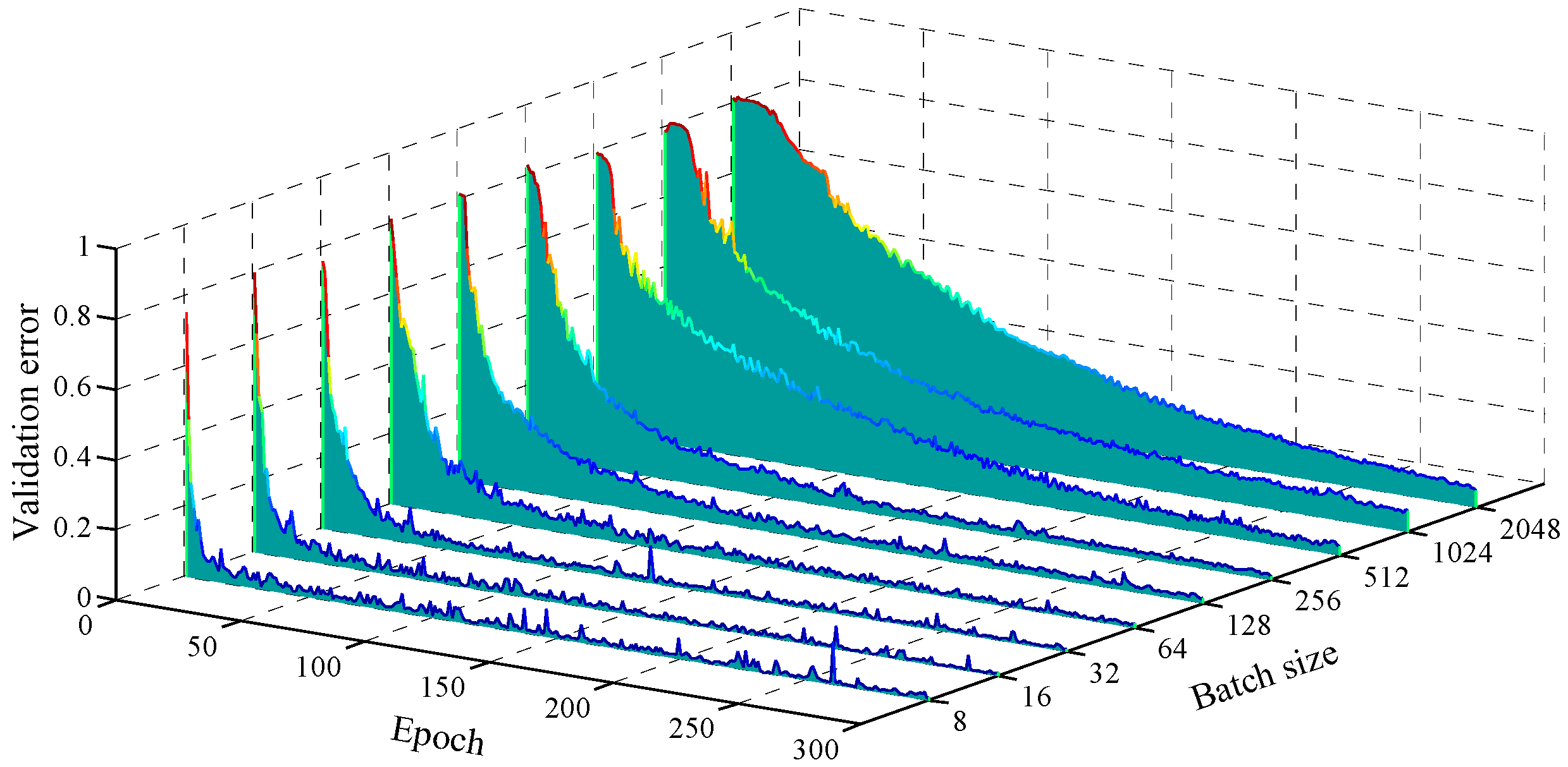
Batch size: Due to the limitations of computer GPU memory, the deep learning model could not process the entire data set at the same time, but split it into multiple batches, making multiple iterations in each epoch. It is necessary to select a suitable batch with a consideration of various factors such as the data set size, single sample size, feature variability and computing power. For the data set in the text, when using different batches, the test error, loss value and training time in the convergence process are shown in Figure 13, Figure 14 and Figure 15. When the batch is very small, fewer samples can be referenced when the model weight is corrected after each iteration, and the global estimation is inaccurate, so that the convergence process is unstable. As shown in Figure 13, when the batch size was no more than 256, the model was basically stable after the 200th epoch. Figure 14 shows the standard deviation of validation errors and validation loss values between the 201st and 300th epochs when using different batch sizes. When the batch size was 256, the standard deviation of the two indicators was the smallest and the convergence process was the most stable. At the same time, the sample matrix in the GPU memory was small, and the acceleration effect of the GPU linear algebra library was not obvious. As the batch size increased, the stability of the convergence process was enhanced. The parallelization multiplication capability of GPU memory was also fully utilized, effectively improving the calculation speed of each epoch. On the other hand, as shown in Figure 15, as the batch size increased, the epoch required to achieve the same accuracy increased, and the efficiency of the entire learning process decreased. Considering the learning efficiency, convergence stability and learning accuracy, the batch size in this paper was determined to be 256.
Learning rate: The error and the learning rate together determine the adjustment of the model weight after each iteration. An ideal learning process is that the convergence curve of loss values falls smoothly and eventually converges to a small residual error. There is an optimal learning rate for a specific task and data set. The higher learning rate allows the model to be quickly adjusted. However, an excessive learning rate will cause the model to deviate in terms of the objective loss function, the convergence curve becomes unstable, the oscillations intensify and even the convergence cannot be achieved. Shrinking the learning rate result into less adjustment of the model parameters after each iteration, which is beneficial to smoothing the convergence curve and is beneficial to reduce the final residual error, but also significantly reduces the convergence speed of the model [57,58,59]. Using the previously optimized model structure and batch size, the results of the ten-fold crossover experiment using different learning rates are shown in Figure 16. It can be seen that increasing the learning rate in a certain range could accelerate the convergence speed of the model. However, an excessive learning rate could also cause the convergence curve of validation accuracy to be unstable or even could not converge. In the end, this article set the learning rate to 0.003.
5. Results and Discussion
5.1. The Advantages of the Spectrum in Training Neural Networks
Zhang W. trains 1-D CNN based on temporal signals to identify bearing faults [60]. There are initial phase differences between the temporal samples, which will interfere with the learning process of CNN. Therefore, the spectrum of the signal was utilized as the input of CNN in this paper. In this section, we will conduct an experimental study of the performance of these two methods of training CNN.
A 1-D temporal data set and a 1-D spectral data set were respectively created based on the reconstructed temporal signal and spectrum of the frequency band . Then, a normalized 1-D temporal data set and a normalized 1-D spectral data set were respectively created by normalization processing. The depth of the 1-D CNN model used was the same as the depth of the previously optimized 2-D CNN model. The size and number of convolution kernels in each layer were set with reference to published literature and optimized using the process described above. The optimized model hyperparameters are listed in Table 2, and the specific optimization process will not be described in detail.
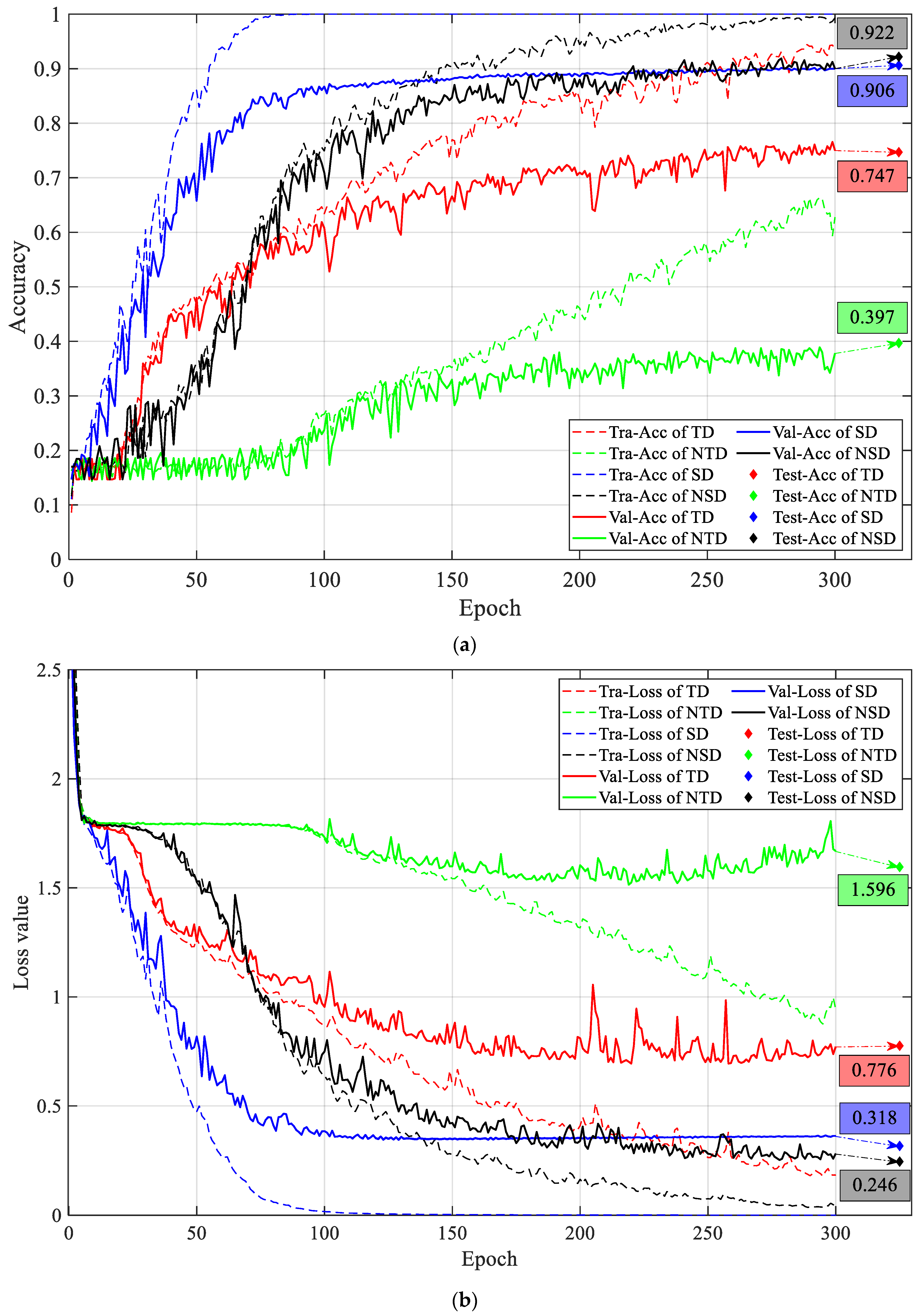
The data sets were randomly divided to the training set, validation set and test set by a ratio of 3:1:1. The result is shown in Figure 17, where TD means the temporal data set, NTD means the normalized temporal data set, SD means the spectral data set and NSD means the normalized spectral data set. Tra-Acc denotes training accuracy, Val-Acc denotes validation accuracy and Test-Acc denotes test accuracy. Tra-Loss denotes training loss value, Val-Loss denotes validation loss value and Test-Loss denotes test loss value.
As the tool wears, the mechanism of the cutting edge removing material gradually changed, and the vibration state of the spindle changed accordingly. The vibration signal records the tool wear process. As can be seen from Figure 17, the 1-D CNN could extract effective features from the spindle vibration signal. The test accuracy of the model trained with the temporal data set was 74.7%. For a 6-class problem, this was far beyond the accuracy of a random decision. Transforming the temporal signal to the frequency domain eliminated the interference of the initial phase of the signal sample on the classification process. The trained model had a test accuracy of 90%, which made it more informative for industrial sites.
The normalization process reduced the discrimination of temporal signals, but the test accuracy of the spectral data set was improved, and the test loss value was also significantly reduced. When the neural network was trained with the unnormalized segment spectrum data set, from the 50th epoch, the training accuracy was significantly higher than the validation accuracy, which means the model began to over fit. At the 100th epoch, the training accuracy had stabilized at 100%, and the validation accuracy reached a steady state, but not more than 90%. The unnormalized spectrum retained the intensity information of the vibration signal, which was the parameter most directly related to the sharpness of the cutting edge, which was also the parameter most tightly related to the cutting conditions. Therefore, when using it to train a neural network, the model could converge quickly; nevertheless, it was also easier to over fit. Normalization could cancel out the intensity information, forcing the model to mine the variation of the spectrum shape and enhance the generalization of the model. In summary, converting the original signal to the frequency domain and normalizing it was most beneficial to the neural network model. The test accuracy was 92.2%, and the test loss value was 0.246.
5.2. Performance Comparison between 1D CNN and 2D CNN
In order to verify the applicability of these two models to this subject, 100 1-D CNNs and 100 2-D CNNs were trained with 100 epochs, respectively, using the 1-D and 2-D normalized spectral data set based on the sub band. The data set was re-randomly divided by a ratio of 3:1:1 each time. The results of the repeated tests are shown in Figure 18 below.
Whether in terms of recognition accuracy or stability, the performance of 2-D CNN was significantly better than 1-D CNN. Although we could not find any specific shape features with the naked eye. The experimental results show that after training, 2-D CNN could learn effective features from 2D map and achieve better recognition accuracy than 1-D CNN. In a 1-D CNN, if the length of the feature vector in a certain convolution layer was , and the length of the filter was . Then, in the convolution operation, there were at most elements that could be associated with the element in the feature vector. If the feature vector was folded into a feature map of , and the size of the 2-D filter was set to . In the 2-D convolution operation, the elements that could be associated with the element were at most . Therefore, when the 2-D filter was the same as the 1-D filter in size, the 2-D convolution operation could make the elements in the feature map establish a wider relationship with each other. More importantly, because the 2-D filter spans multiple lines, the relation scope was broader. Therefore, in this paper, although the total parameters of the 1-D CNN were more than twice that of the 2-D CNN, the learning ability was still far less than the latter.
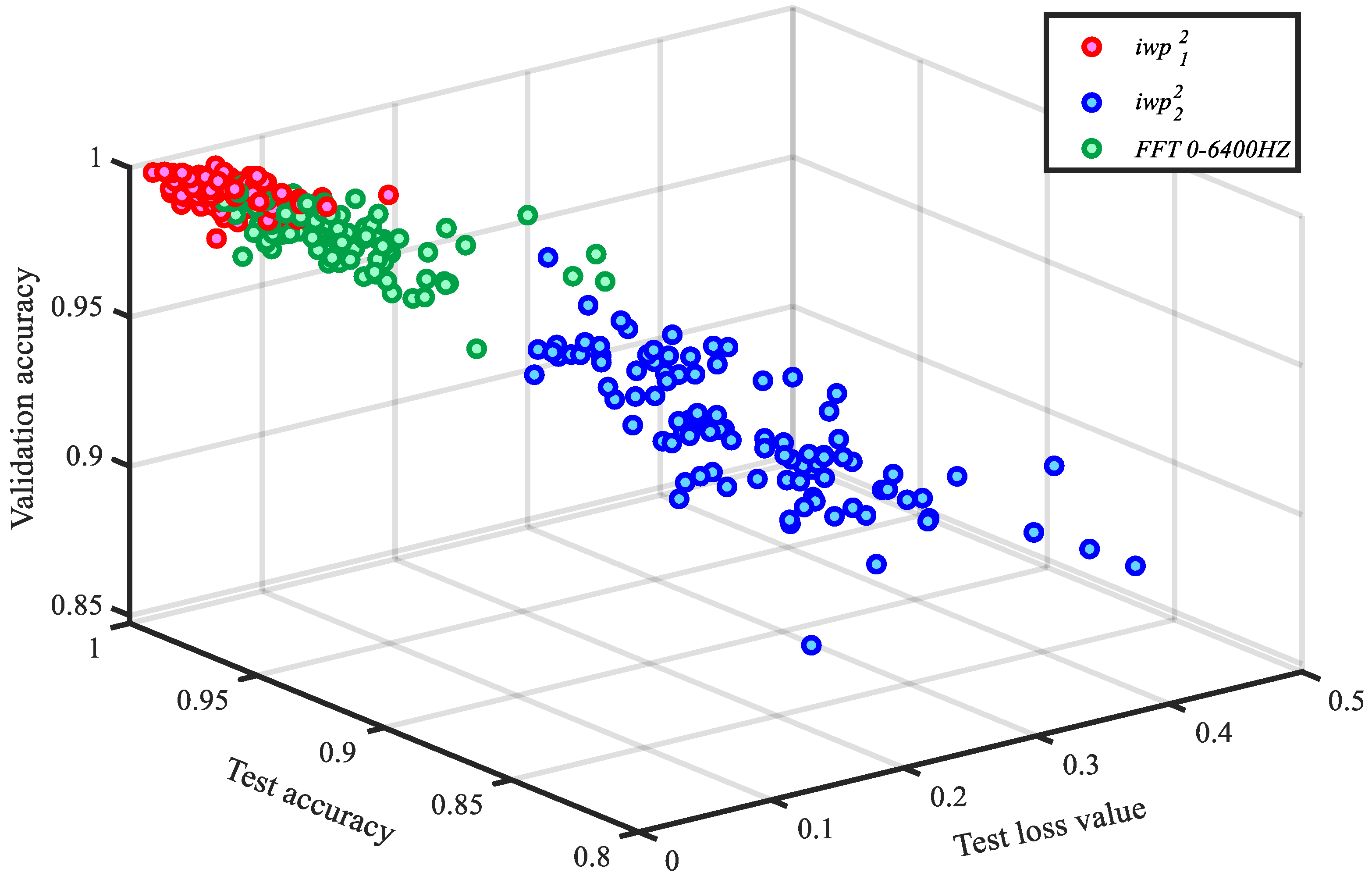
5.3. DWFs’ Optimization of the Sample
As described in Section 3.3, two bands containing more transient impact information, and , were extracted using the DWFs algorithm. Two data sets were created based on the spectra of the two sub-spectrum, respectively. In order to verify the beneficial effects of the DWFs, this paper also created a 2-D data set based on the complete fast Fourier transform spectrum of the raw 1-D sample. Its frequency band was , which was twice that of . Repeated modeling experiments were performed 100 times with 100 epochs, and the results are shown in Figure 19. It can be seen that the effect of the frequency band was obviously less than that of and the full spectrum. Although the bandwidth of this band was narrower, more noise could be filtered out, and the impact characteristics were more prominent in the time domain. However, the impact forms of the cutting edge and the work piece were similar under different degrees of wear. After normalizing the spectrum, only the information retained in this narrow frequency band might be insufficient. had improved performance compared to the full spectrum. This might be due to the elimination of interference from other frequency bands, especially the noise in the high frequency band and the steady state signal in the low frequency band. More notably, was reduced by half compared to the full spectrum calculation, which significantly improved the recognition speed of the model.
5.4. The Effectiveness of the Proposed Methodology
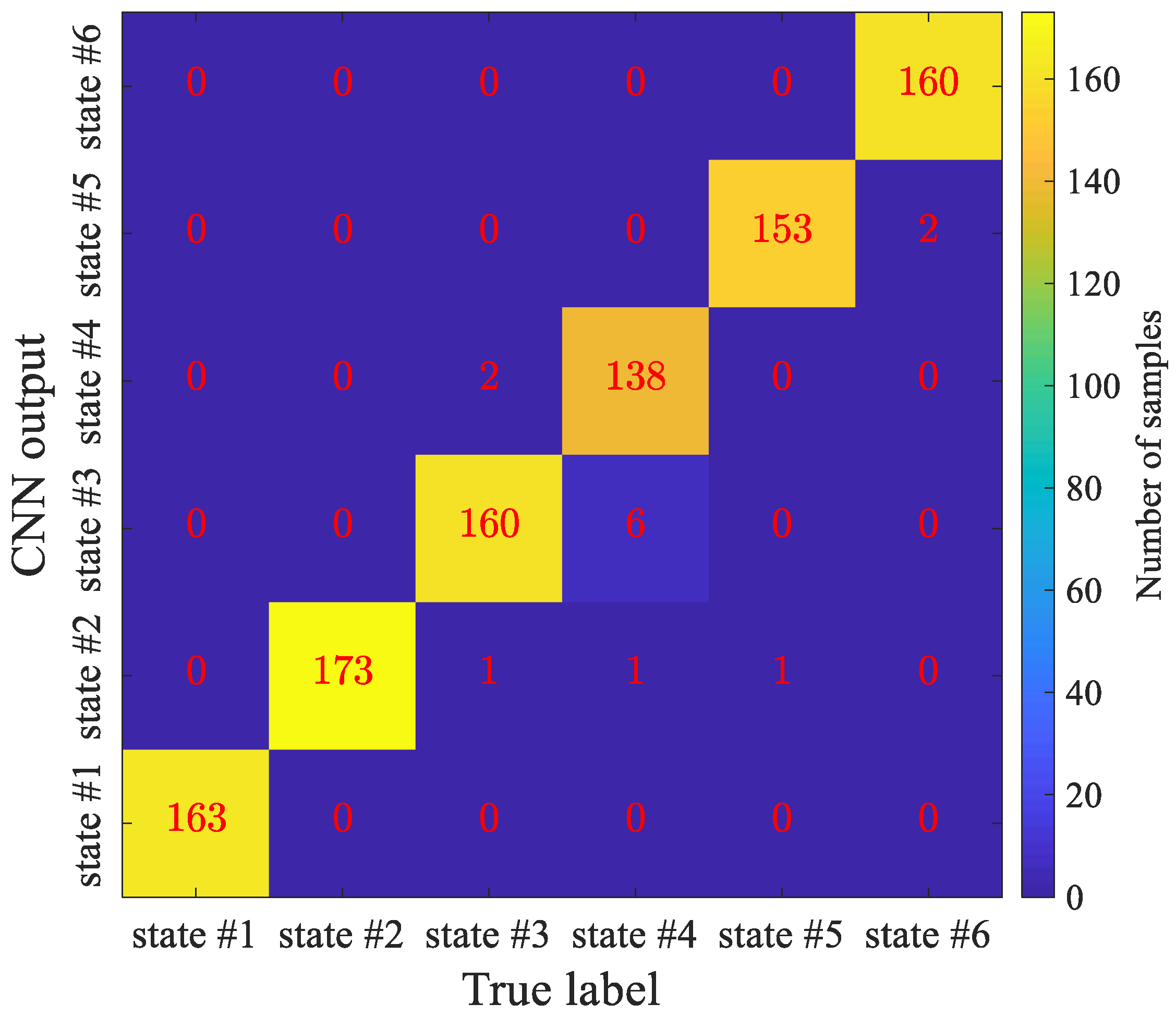
Finally, the band normalized spectrum in 2-D format was used as the input of the 2-D CNN. The data set with a total sample size of 4800 was randomly divided into the training set, validation set and test set. The convolutional neural network was trained with the first two subsets, with 150 epochs. After the training was completed, the model’s recognition ability was tested with the test set that was not involved in the training process. The test accuracy was 98.65%, and the confusion matrix of the recognition results is shown in Figure 20. The confusion matrix was an effective visualization tool to estimate the performance of classification algorithm. Each element in the matrix represents a type of sample. The abscissa of the element is the real label of the sample. The ordinate of the element is the label of the CNN output. The value of the element is the number of such elements.
As can be seen from the figure, the recognition accuracy of all these six types was fairly high. The recognition accuracy of the fourth type (tool wear state label is state #4) was relatively low, but it also reached 95.2%, which met the requirements of the manufacturing site, which proved the effectiveness of the method given in this paper.
6. Conclusions
This paper expanded the application of 2-D CNN in the field of tool wear state identification. The raw signal was decomposed with constant power via DWFs. Then the frequency band with more impulsive components and higher signal-to-noise ratio was selected according to the kurtosis of the reconstructed sub-signal. Further, the 1-D spectrum was folded into 2-D spectral map. After converting the spectrum of the sample signal in different wear states into normalized 2-D maps, no significant difference characteristics could be found by visual observation. Therefore, the CNN model was trained to extract features from the 2-D map and achieve good classification accuracy. The deep convolutional neural network could adaptively extract implicit features from large input data. However, in the spindle vibration signal, the information on tool wear was interfered by other contents. The feature engineering based on DWFs constructed a better data set for CNN, and thus significantly improved the learning speed and recognition accuracy of CNN.
In high-automation workshops that perform small-batch production, a milling tool often participates in the processing of different products. At this industrial site, the number of machined parts is not sufficient to accurately predict the remaining life of the milling tool. The experimental results show that the proposed method could indirectly monitor the wear state of the milling tool based on the spindle vibration signal. Even if the cutting conditions were unknown when acquiring signals, the wear state of the milling tool could still be accurately recognized. The 2-D CNN model constructed in this paper contained a total of 24,306 trainable parameters. After the CNN model was trained, the time cost of one sample was less than 0.005 s, while the data processing based on DWFs took about 0.13 s. Coupled with data acquisition and transmission time, the total time cost to perform a tool wear state recognition was less than 1.5 s, which basically met the requirements of online monitoring. Some conclusions could be drawn as follows:
- (1)
- The impact of the cutting edge and the work piece was the main stimulus for the machine shaft vibration. As the sharpness of the cutting edge gradually decreased, the vibration mode of the spindle changed. The vibration acceleration data indirectly recorded the wear process of the tool. The 1-D CNN could extract implicit features from it, nevertheless, the test accuracy was only 75%. There were many interfering contents in the raw signal, and changes in cutting conditions interfered with the neural network, so proper feature engineering was indispensable.
- (2)
- Transforming the signal from the time domain to the frequency domain eliminated the interference of the initial phase on the neural network when the signal was acquired. Normalization could reduce the dependence of neural networks on signal strength, forcing them to mine features that were less relevant to cutting conditions. Using the normalized spectrum to train 1-D CNN, the test recognition accuracy reached 92%, which was obviously better than the temporal signal.
- (3)
- Folding the 1-D spectra into 2-D spectral maps gave full play to the more powerful learning ability of the 2-D CNN. The 1600–4800 Hz frequency band selected by the DWFs algorithm had a higher signal-to-noise ratio, which reduced the size of the input to CNN by half, and further improved the recognition accuracy of the neural network model, reaching 98.6%.
The tool wear condition monitoring method proposed in this paper could also be used for other machining methods, such as drilling and turning. The method to identify the state of the monitoring signal using a 2-D CNN might also be extended to other fault diagnosis occasions, such as gear fault diagnosis based on vibration signals.
Author Contributions
Conceptualization, X.C. and B.C.; methodology, B.Y.; software, X.C.; validation, X.C. and B.C.; formal analysis, B.Y.; investigation, B.C.; resources, B.Y.; data curation, B.C.; writing—original draft preparation, X.C.; writing—review and editing, B.C.; visualization, X.C.; supervision, S.Z.; project administration, S.Z.; funding acquisition, B.C.
Funding
This research is supported financially by National Natural Science Foundation of China (No. 51605403); Natural Science Foundation of Guangdong Province, China (No. 2015A030310010); Natural Science Foundation of Fujian Province, China (No. 2016J01012); Aeronautical Science Foundation of China (20183368004); and the Fundamental Research Funds for the Central Universities under Grant (20720190009).
Conflicts of Interest
The authors declare no conflict of interest.
References
- Klocke, F.; Eisenblätter, G. Dry cutting. CIRP Ann. 1997, 46, 519–526. [Google Scholar] [CrossRef]
- Dutta, S.; Pal, S.K.; Sen, R. Tool condition monitoring in turning by applying machine vision. J. Manuf. Sci. Eng. 2016, 138, 051008. [Google Scholar] [CrossRef]
- Siddhpura, A.; Paurobally, R. A review of flank wear prediction methods for tool condition monitoring in a turning process. Int. J. Adv. Manuf. Technol. 2013, 65, 371–393. [Google Scholar] [CrossRef]
- Wang, W.; Hong, G.; Wong, Y.; Zhu, K. Sensor fusion for online tool condition monitoring in milling. Int. J. Prod. Res. 2007, 45, 5095–5116. [Google Scholar] [CrossRef]
- Kamarthi, S.; Kumara, S.; Cohen, P. Flank wear estimation in turning through wavelet representation of acoustic emission signals. J. Manuf. Sci. Eng. 2000, 122, 12–19. [Google Scholar] [CrossRef]
- Lu, M.-C.; Kannatey-Asibu, E. Analysis of sound signal generation due to flank wear in turning. J. Manuf. Sci. Eng. 2002, 124, 799–808. [Google Scholar] [CrossRef]
- Axinte, D.A. Approach into the use of probabilistic neural networks for automated classification of tool malfunctions in broaching. Int. J. Mach. Tools Manuf. 2006, 46, 1445–1448. [Google Scholar] [CrossRef]
- Chudzikiewicz, A.; Bogacz, R.; Kostrzewski, M.; Konowrocki, R. Condition monitoring of railway track. Transport 2018, 33, 33–42. [Google Scholar]
- Byrne, G.; Dornfeld, D.; Denkena, B. Advancing cutting technology. CIRP Ann. 2003, 52, 483–507. [Google Scholar] [CrossRef]
- Nouri, M.; Fussell, B.K.; Ziniti, B.L.; Linder, E. Real-time tool wear monitoring in milling using a cutting condition independent method. Int. J. Mach. Tools Manuf. 2015, 89, 1–13. [Google Scholar] [CrossRef]
- Liu, C.; Li, Y.; Zhou, G.; Shen, W. A sensor fusion and support vector machine based approach for recognition of complex machining conditions. J. Intell. Manuf. 2018, 29, 1739–1752. [Google Scholar] [CrossRef]
- Jose, B.; Nikita, K.; Patil, T.; Hemakumar, S.; Kuppan, P. Online Monitoring of Tool Wear and Surface Roughness by using Acoustic and Force Sensors. Mater. Today Proc. 2018, 5, 8299–8306. [Google Scholar] [CrossRef]
- Krishnakumar, P.; Rameshkumar, K.; Ramachandran, K. Acoustic Emission-Based Tool Condition Classification in a Precision High-Speed Machining of Titanium Alloy: A Machine Learning Approach. Int. J. Comput. Intell. Appl. 2018, 17, 1850017. [Google Scholar] [CrossRef]
- Niaki, F.A.; Michel, M.; Mears, L. State of health monitoring in machining: Extended Kalman filter for tool wear assessment in turning of IN718 hard-to-machine alloy. J. Manuf. Process. 2016, 24, 361–369. [Google Scholar] [CrossRef] [Green Version]
- Madhusudana, C.; Kumar, H.; Narendranath, S. Face milling tool condition monitoring using sound signal. Int. J. Syst. Assur. Eng. Manag. 2017, 8, 1643–1653. [Google Scholar] [CrossRef]
- Nakandhrakumar, R.; Dinakaran, D.; Pattabiraman, J.; Gopal, M. Tool flank wear monitoring using torsional—Axial vibrations in drilling. Prod. Eng. 2019, 13, 107–118. [Google Scholar] [CrossRef]
- Mohanraj, T.; Shankar, S.; Rajasekar, R.; Deivasigamani, R.; Arunkumar, P.M. Tool condition monitoring in the milling process with vegetable based cutting fluids using vibration signatures. Mat. Test. 2019, 61, 282–288. [Google Scholar] [CrossRef]
- Yan, R.; Li, X.; Chen, Z.; Xu, Q.; Chen, X. Improving calibration accuracy of a vibration sensor through a closed loop measurement system. IEEE Instrum. Measur. Mag. 2016, 19, 42–46. [Google Scholar] [CrossRef]
- Du, Z.; Chen, X.; Zhang, H.; Yang, B.; Zhai, Z.; Yan, R. Weighted low-rank sparse model via nuclear norm minimization for bearing fault detection. J. Sound Vib. 2017, 400, 270–287. [Google Scholar] [CrossRef]
- Segreto, T.; Simeone, A.; Teti, R. Principal component analysis for feature extraction and NN pattern recognition in sensor monitoring of chip form during turning. CIRP J. Manuf. Sci. Technol. 2014, 7, 202–209. [Google Scholar] [CrossRef]
- He, W.; Ding, Y.; Zi, Y.; Selesnick, I.W. Repetitive transients extraction algorithm for detecting bearing faults. Mech. Syst. Sig. Process. 2017, 84, 227–244. [Google Scholar] [CrossRef] [Green Version]
- Fu, Y.; Zhang, Y.; Gao, H.; Mao, T.; Zhou, H.; Sun, R.; Li, D. Automatic feature constructing from vibration signals for machining state monitoring. J. Intell. Manuf. 2019, 30, 995–1008. [Google Scholar] [CrossRef]
- Segreto, T.; Caggiano, A.; Karam, S.; Teti, R. Vibration sensor monitoring of nickel-titanium alloy turning for machinability evaluation. Sensors 2017, 17, 2885. [Google Scholar] [CrossRef] [PubMed]
- He, W.; Chen, B.; Zeng, N.; Zi, Y. Sparsity-based signal extraction using dual Q-factors for gearbox fault detection. ISA Trans. 2018, 79, 147–160. [Google Scholar] [CrossRef] [PubMed]
- Kurek, J.; Kruk, M.; Osowski, S.; Hoser, P.; Wieczorek, G.; Jegorowa, A.; Górski, J.; Wilkowski, J.; Śmietańska, K.; Kossakowska, J. Developing automatic recognition system of drill wear in standard laminated chipboard drilling process. Bull. Pol. Acad. Sci. Tech. Sci. 2016, 64, 633–640. [Google Scholar] [CrossRef] [Green Version]
- Hong, Y.-S.; Yoon, H.-S.; Moon, J.-S.; Cho, Y.-M.; Ahn, S.-H. Tool-wear monitoring during micro-end milling using wavelet packet transform and Fisher’s linear discriminant. Int. J. Precis. Eng. Manuf. 2016, 17, 845–855. [Google Scholar] [CrossRef]
- Martins, C.H.R.; Aguiar, P.R.; Frech, A.; Bianchi, E.C. Tool Condition Monitoring of Single-Point Dresser Using Acoustic Emission and Neural Networks Models. IEEE Instrum. Measur. Mag. 2014, 63, 667–679. [Google Scholar] [CrossRef]
- Wang, G.; Guo, Z.; Lei, Q. Online incremental learning for tool condition classification using modified Fuzzy ARTMAP network. J. Intell. Manuf. 2014, 25, 1403–1411. [Google Scholar] [CrossRef]
- Geramifard, O.; Xu, J.X.; Zhou, J.H.; Li, X. Multimodal Hidden Markov Model-Based Approach for Tool Wear Monitoring. IEEE Trans. Ind. Electron. 2014, 61, 2900–2911. [Google Scholar] [CrossRef]
- Jain, A.K.; Lad, B.K. A novel integrated tool condition monitoring system. J. Intell. Manuf. 2019, 30, 1423–1436. [Google Scholar] [CrossRef]
- Wang, G.; Yang, Y.; Xie, Q.; Zhang, Y. Force based tool wear monitoring system for milling process based on relevance vector machine. Adv. Eng. Softw. 2014, 71, 46–51. [Google Scholar] [CrossRef]
- Wang, G.; Yang, Y.; Guo, Z. Hybrid learning based Gaussian ARTMAP network for tool condition monitoring using selected force harmonic features. Sens. Actuators A Phys. 2013, 203, 394–404. [Google Scholar] [CrossRef]
- Tobon-Mejia, D.A.; Medjaher, K.; Zerhouni, N. CNC machine tool’s wear diagnostic and prognostic by using dynamic Bayesian networks. Mech. Syst. Signal. Process. 2012, 28, 167–182. [Google Scholar] [CrossRef]
- Krizhevsky, A.; Sutskever, I.; Hinton, G.E. Imagenet classification with deep convolutional neural networks. Adv. Neural Inf. Process. Syst. 2012, 25, 1097–1105. [Google Scholar] [CrossRef]
- Zhu, Y.; Zhang, C.; Zhou, D.; Wang, X.; Bai, X.; Liu, W. Traffic sign detection and recognition using fully convolutional network guided proposals. Neurocomputing 2016, 214, 758–766. [Google Scholar] [CrossRef]
- Kim, Y. Convolutional neural networks for sentence classification. arXiv 2014, arXiv:1408.5882. [Google Scholar]
- Palaz, D.; Collobert, R.; Doss, M.M. Estimating phoneme class conditional probabilities from raw speech signal using convolutional neural networks. arXiv 2013, arXiv:1304.1018. [Google Scholar]
- Sun, W.; Yao, B.; Zeng, N.; Chen, B.; He, Y.; Cao, X.; He, W. An Intelligent Gear Fault Diagnosis Methodology Using a Complex Wavelet Enhanced Convolutional Neural Network. Materials 2017, 10, 790. [Google Scholar] [CrossRef] [PubMed]
- Wang, F.; Jiang, H.; Shao, H.; Duan, W.; Wu, S. An adaptive deep convolutional neural network for rolling bearing fault diagnosis. Measur. Sci. Tech. 2017, 28, 9. [Google Scholar]
- Chen, L.; Wang, Z.; Zhou, B. Intelligent fault diagnosis of rolling bearing using hierarchical convolutional network based health state classification. Adv. Eng. Inf. 2017, 32, 139–151. [Google Scholar]
- Fu, Y.; Zhang, Y.; Gao, Y.; Gao, H.; Mao, T.; Zhou, H.; Li, D. Machining vibration states monitoring based on image representation using convolutional neural networks. Eng. Appl. Artif. Intell. 2017, 65, 240–251. [Google Scholar] [CrossRef]
- He, W.; Ding, Y.; Zi, Y.; Selesnick, I.W. Sparsity-based algorithm for detecting faults in rotating machines. Mech. Syst. Sig. Process. 2016, 72, 46–64. [Google Scholar] [CrossRef]
- Wang, Y.; He, Z.; Zi, Y. Enhancement of signal denoising and multiple fault signatures detecting in rotating machinery using dual-tree complex wavelet transform. Mech. Syst. Signal. Process. 2010, 24, 119–137. [Google Scholar] [CrossRef]
- Selesnick, I.W.; Baraniuk, R.G.; Kingsbury, N.G. The dual-tree complex wavelet transform. IEEE Signal. Process. Mag. 2005, 22, 123–151. [Google Scholar] [CrossRef] [Green Version]
- Yan, R.; Gao, R.X.; Chen, X. Wavelets for fault diagnosis of rotary machines: A review with applications. Signal. Process. 2014, 96, 1–15. [Google Scholar] [CrossRef]
- Chen, B.; Zhang, Z.; Yanyang, Z.I.; Zhengjia, H.E. Novel Ensemble Analytic Discrete Framelet Expansion for Machinery Fault Diagnosis. J. Mech. Eng. 2014, 50, 77. [Google Scholar] [CrossRef]
- Cao, X.-C.; Chen, B.-Q.; Yao, B.; He, W.-P. Combining translation-invariant wavelet frames and convolutional neural network for intelligent tool wear state identification. Comput. Ind. 2019, 106, 71–84. [Google Scholar] [CrossRef]
- Yang, W.; Jin, L.; Tao, D.; Xie, Z.; Feng, Z. DropSample: A new training method to enhance deep convolutional neural networks for large-scale unconstrained handwritten Chinese character recognition. Pattern Recognit. 2016, 58, 190–203. [Google Scholar] [CrossRef]
- Boureau, Y.L.; Ponce, J.; Lecun, Y. A Theoretical Analysis of Feature Pooling in Visual Recognition. In Proceedings of the 27th International Conference on Machine Learning, Haifa, Israel, 21–25 June 2010; pp. 111–118. [Google Scholar]
- Lian, Z.; Jing, X.; Wang, X.; Huang, H.; Tan, Y.; Cui, Y. DropConnect regularization method with sparsity constraint for neural networks. Chin. J. Electron. 2016, 25, 152–158. [Google Scholar] [CrossRef]
- Borghesani, P.; Pennacchi, P.; Chatterton, S. The relationship between kurtosis-and envelope-based indexes for the diagnostic of rolling element bearings. Mech. Syst. Sig. Process. 2014, 43, 25–43. [Google Scholar] [CrossRef]
- Obuchowski, J.; Wyłomańska, A.; Zimroz, R. Selection of informative frequency band in local damage detection in rotating machinery. Mech. Syst. Sig. Process. 2014, 48, 138–152. [Google Scholar] [CrossRef]
- Rubinstein, R. The cross-entropy method for combinatorial and continuous optimization. Method. Comput. Appl. Probab. 1999, 1, 127–190. [Google Scholar] [CrossRef]
- Shang, L.; Yang, Q.; Wang, J.; Li, S.; Lei, W. Detection of rail surface defects based on CNN image recognition and classification. In Proceedings of the 20th International Conference on Advanced Communication Technology (ICACT), Chuncheon-si, Gangwon-do, South Korea, 11–14 February 2018; pp. 45–51. [Google Scholar]
- Kline, D.M.; Berardi, V.L. Revisiting squared-error and cross-entropy functions for training neural network classifiers. Neural Comput. Appl. 2005, 14, 310–318. [Google Scholar] [CrossRef]
- Kingma, D.P.; Ba, J. Adam: A method for stochastic optimization. arXiv 2014, arXiv:1412.6980. [Google Scholar]
- Goodfellow, I.; Bengio, Y.; Courville, A. Deep Learning; MIT Press: Cambridge, MA, USA, 2016. [Google Scholar]
- Darken, C.; Moody, J.E. Note on Learning Rate Schedules for Stochastic Optimization. In Advances in Neural Information Processing Systems; Lippmann, R., Moody, J., Touretzky, D.S., Eds.; Morgan Kaufmann: San Mateo, CA, USA, 1991; pp. 832–838. [Google Scholar]
- Zeiler, M.D. ADADELTA: An adaptive learning rate method. arXiv 2012, arXiv:1212.5701. [Google Scholar]
- Zhang, W.; Li, C.; Peng, G.; Chen, Y.; Zhang, Z. A deep convolutional neural network with new training methods for bearing fault diagnosis under noisy environment and different working load. Mech. Syst. Sig. Process. 2018, 100, 439–453. [Google Scholar] [CrossRef]
Figure 1.
Filter-bank structure of the dual tree wavelet packet decomposition.

Figure 2.
Hybrid wavelet bases of dual tree complex wavelet packet decomposition. (a) Scaling function of Symlet10; (b) wavelet function of Symlet10; (c) complex scaling function of Q-Shift20 and (d) complex wavelet function of Q-Shift20.
Figure 2.
Hybrid wavelet bases of dual tree complex wavelet packet decomposition. (a) Scaling function of Symlet10; (b) wavelet function of Symlet10; (c) complex scaling function of Q-Shift20 and (d) complex wavelet function of Q-Shift20.

Figure 3.
Frequency-scale paving of derived wavelet frames (DWFs).

Figure 4.
The basic architecture of the convolutional neural network (CNN) model.

Figure 5.
Illustration of different CNN components: (a) Convolution layer; (b) ReLU unit and (c) pooling layer.
Figure 5.
Illustration of different CNN components: (a) Convolution layer; (b) ReLU unit and (c) pooling layer.

Figure 6.
Illustration of the (a) flatten layer, (b) fully connected layer and (c) dropout network.

Figure 7.
Flow chart of the proposed method.

Figure 8.
The kurtosis map of the vibration signal after being decomposed via derived wavelet frames (DWFs), where “CoCC” means the combination of cutting conditions and “TWS” means the tool wear state.
Figure 8.
The kurtosis map of the vibration signal after being decomposed via derived wavelet frames (DWFs), where “CoCC” means the combination of cutting conditions and “TWS” means the tool wear state.

Figure 9.
Validation accuracy convergence curves of different structural neural network models.

Figure 10.
Training results of neural network models with different structures.

Figure 11.
Performance for different combinations of the number of neurons in the first full connection layer and dropout rate in terms of the (a) average test accuracy and (b) average test loss value.
Figure 11.
Performance for different combinations of the number of neurons in the first full connection layer and dropout rate in terms of the (a) average test accuracy and (b) average test loss value.

Figure 12.
The architecture of the CNN model used in this paper, where “Conv2d_1 (12-5*5)” refers to the first convocation layer consists of 12 filters with a size of 5*5, “MaxPooling (2*2)” refers to max pooling layer with a pooling size of 2*2.
Figure 12.
The architecture of the CNN model used in this paper, where “Conv2d_1 (12-5*5)” refers to the first convocation layer consists of 12 filters with a size of 5*5, “MaxPooling (2*2)” refers to max pooling layer with a pooling size of 2*2.

Figure 13.
The effect of the batch size on the convergence process of the validation error.

Figure 14.
The standard deviation of the validation error and validation loss value after the model was stabilized.
Figure 14.
The standard deviation of the validation error and validation loss value after the model was stabilized.

Figure 15.
The effect of batch size on the calculation time cost of a single epoch and the speed of model learning.
Figure 15.
The effect of batch size on the calculation time cost of a single epoch and the speed of model learning.

Figure 16.
Illustration of the effect of the learning rate on convergence speed and convergence stability of the model.
Figure 16.
Illustration of the effect of the learning rate on convergence speed and convergence stability of the model.

Figure 17.
Performance comparison of time domain and frequency domain in terms of accuracy (a) and the loss value (b).
Figure 17.
Performance comparison of time domain and frequency domain in terms of accuracy (a) and the loss value (b).

Figure 18.
Performance comparison between 1-D CNN and 2-D CNN.

Figure 19.
Performance comparison of data sets constructed with different frequency bands.

Figure 20.
Confusion matrix.


Table 1.
Cutting conditions.
| Combination of Cutting Conditions | Milling Pass | Radial Cutting Depth (mm) | Axial Cutting Depth (mm) | Feed Per Tooth (mm) | Spindle Speed (r/min) |
|---|---|---|---|---|---|
| # 1 | 1–4 | 1 | 5 | 0.08 | 800 |
| # 2 | 5–8 | 2.5 | 5 | 0.06 | 800 |
| # 3 | 9–12 | 1 | 5 | 0.08 | 1200 |
| # 4 | 13–16 | 2.5 | 5 | 0.06 | 1200 |
Table 2.
Model structure of the employed 1D CNN.
| Layer Name | Filter Number | Filter Size | Activation |
|---|---|---|---|
| Conv1D_1 | 16 | 64*1 | ReLU |
| MaxPooling1D_1 | ---- | 8*1 | ReLU |
| Conv1D_2 | 32 | 32*1 | ReLU |
| MaxPooling1D_2 | ---- | 4*1 | ReLU |
| Conv1D_3 | 64 | 16*1 | ReLU |
| MaxPooling1D_3 | ---- | 2*1 | ReLU |
| Conv1D_4 | 128 | 8*1 | ReLU |
| Global-max- -pooling1D_1 | ---- | ---- | ---- |
| Dense_1 | 72 | ---- | ReLU |
| output | 6 | ---- | Softmax |
© 2019 by the authors. Licensee MDPI, Basel, Switzerland. This article is an open access article distributed under the terms and conditions of the Creative Commons Attribution (CC BY) license (http://creativecommons.org/licenses/by/4.0/).
Share and Cite
MDPI and ACS Style
Cao, X.; Chen, B.; Yao, B.; Zhuang, S. An Intelligent Milling Tool Wear Monitoring Methodology Based on Convolutional Neural Network with Derived Wavelet Frames Coefficient. Appl. Sci. 2019, 9, 3912. https://doi.org/10.3390/app9183912
AMA Style
Cao X, Chen B, Yao B, Zhuang S. An Intelligent Milling Tool Wear Monitoring Methodology Based on Convolutional Neural Network with Derived Wavelet Frames Coefficient. Applied Sciences. 2019; 9(18):3912. https://doi.org/10.3390/app9183912
Chicago/Turabian StyleCao, Xincheng, Binqiang Chen, Bin Yao, and Shiqiang Zhuang. 2019. "An Intelligent Milling Tool Wear Monitoring Methodology Based on Convolutional Neural Network with Derived Wavelet Frames Coefficient" Applied Sciences 9, no. 18: 3912. https://doi.org/10.3390/app9183912
Note that from the first issue of 2016, this journal uses article numbers instead of page numbers. See further details here.