Multi-Objective Optimization for Plug-In 4WD Hybrid Electric Vehicle Powertrain

Abstract

This paper focuses on the parameter optimization for the CVT (a continuously variable transmission) based plug-in 4WD (4-wheel drive) hybrid electric vehicle powertrain. First, the plug-in 4WD hybrid electric vehicle (plug-in 4WD HEV)’s energy management strategy based on the CD (charge depleting) and CS (charge sustain) mode is developed. Then, the multi-objective optimization’s mathematical model, which aims at minimizing the electric energy consumption under the CD stage, the fuel consumption under the CS stage and the acceleration time from 0–120 km/h, is established. Finally, the multi-objective parameter optimization problem is solved using an evolutionary based non-dominated sorting genetic algorithms-II (NSGA-II) approach. Some of the results are compared with the original scheme and the classical weight approach. Compared with the original scheme, the best compromise solution (i.e., electric energy consumption, fuel consumption and acceleration time) obtained using the NSGA-II approach are reduced by 1.21%, 6.18% and 5.49%, respectively. Compared with the weight approach, the Pareto optimal solutions obtained using NSGA-II approach are better distributed over the entire Pareto optimal front, as well as the best compromise solution is also better.

1. Introduction

Owing to regulations on fuel economy and emissions become more and more stringent, the development of electrified vehicles in recent years have been a surging trend [1,2]. Plug-in hybrid electric vehicles (PHEVs), which achieve a longer all-electric range compared to conventional hybrid electric vehicles and have no driver range anxiety compared to pure battery electric vehicles, become an important research direction in the field of electric vehicles [3,4].

The parameters of PHEV’s powertrain have a significant impact on the electric energy consumption, fuel consumption and dynamic performance of the vehicle. Therefore, parameter optimization of the powertrain is the basis of the vehicle development. The research on PHEV’s parameter optimization has gone through the following process. In the initial stage, scholars did not realize the problem that powertrain parameters and control strategy parameters coupled and affected vehicles’ performance together. Therefore, the parameter optimization during this stage is mainly focused on independent optimization of powertrain parameters, instead of joint optimizing the parameters of powertrain and control strategy [5,6]. With the in-depth research, attention has been paid to the coupling problem of powertrain parameters and control strategy parameters. Then, simultaneously optimization of powertrain parameters and control strategy parameters begins to appear in some literature [7,8,9]. Actually, literatures [5,6,7,8,9] take parameter optimization as a single objective optimization problem, the parameters of PHEV are optimized to only improve the economy of the vehicle. However, the objectives of vehicle economy, power system cost, emission and power performance usually conflict with each other. The optimization only considering the vehicle economy will result in achieving optimal economic performance at the expense of other objectives that conflict with it. Therefore, in recent years, multi-objective optimization has been applied to optimize PHEV’s parameters. In reference [10], energy storage system costs and fuel economy are considered as the objective functions for hybrid electric vehicle’s battery size optimization. Reference [11] presents a multi-objective optimization methodology for vehicles design considering the parameters for design and macro level operating strategy. Reference [12] applies multi-objective algorithms (minimization of the couples cost and fuel, cost and LCA (life cycle impact) CO_2eq, fuel and LCA CO_2eq) to perform the powertrain components optimization. Reference [13] takes powertrain cost, fuel consumption and emission as multi-objectives to optimize the parameters of powertrain and control parameters simultaneously. In [14], the usage cost, acceleration performance and mode discrimination of the whole vehicle under a new European driving cycle (NEDC) are considered as the optimization objectives to optimize the transmission system of a new hybrid power system. Reference [15] aims at minimizing the cost of the power supply and the energy flow of batteries, and adopts the convex optimization algorithm to optimize the power supply’s parameters and energy management strategy.

Multi-objective optimization and its applications have been an important area of research for over two decades now [16]. The key of solving the multi-objective optimization problem is how to get the Pareto solution set. Traditional algorithms for solving multi-objective optimization problems include the linear weighting method [17], constraint method [18], mini–max method [19], goal programming method [20] and goal satisfaction method [21]. In order to get the Pareto solution set, these methods need to run many times, which reduces the efficiency of the algorithm. Evolutionary algorithms are a group-based global optimization algorithm that simulate the evolution process of natural organisms [22]. The evolutionary algorithm has achieved great success in solving power system’s multi-objective optimization problems [16,23,24,25], e.g., a strength Pareto evolutionary algorithm is used to solve the multi-objective reactive power price clearing problem [23]; a novel-efficient evolutionary-based multi-objective optimization approach is proposed to solve multi-objective optimal power flow problems [16,24] and the multi-objective strength Pareto evolutionary algorithm 2+ has been employed to solve the congestion management problem [25]. Therefore, it has become an important method for solving multi-objective optimization problems.

Parameter optimization of PHEVs is related to the energy management strategy, and energy management strategies need to be developed before parameter optimization. At present, the research on the energy management strategy for PHEVs mainly focuses on the development of the advanced optimization algorithm, such as the algorithm based on the minimum equivalent fuel consumption [26,27,28,29], the dynamic programming algorithm [30,31,32], stochastic dynamic programming [33], the algorithm based on convex optimization [2,34] and the model predictive control algorithm [35,36,37,38]. Although the above-mentioned optimization algorithm can obtain the local or global optimum, it is difficult to apply to real vehicle control for hardly knowing the driving cycles beforehand or the large amount of calculation. However, the rule control strategy based on the charge depleting–charge sustain (CD–CS) mode does not need to know the driving cycles beforehand, and the calculation is small, so it is widely used in the real vehicle control of PHEVs.

As a summary of the entire literature review, in order to complete the plug-in 4WD HEV’s parameter optimization well, the simultaneous optimization for the main parameters of powertrain and control strategy is necessary, multi-objective optimization should be taken into account and the rule control strategy based on the CD–CS mode for plug-in 4WD HEVs should be developed. However, there is still a large shortage for plug-in 4WD HEV’s parameter optimization. Firstly, it is still challenging to select reasonably multi-objective functions, which can evaluate the optimal performance of plug-in 4WD HEV well. Secondly, although the evolutionary algorithm has achieved great success in solving power system’s multi-objective optimization problems, it rarely applies to solve plug-in 4WD HEV’s multi-objective parameter optimization problems. Finally, the rule control strategy based on the CD–CS mode for plug-in 2WD hybrid electric vehicles is mature, but there is little literature on the rule control strategy based on the CD–CS mode for plug-in 4WD HEVs.

To address the challenges summarized above, in this study, the energy management strategy based on the CD–CS mode for plug-in 4WD HEV is developed. Then, the reasonably multi-objective functions, which are composed of electric energy consumption under the CD stage, fuel consumption under the CS stage and acceleration time from 0–120 km/h, are established. Finally, the evolutionary based NSGA-II (non-dominated sorting genetic algorithms-II) approach is selected to simultaneously optimize the parameters of the powertrain and control strategy.

The outline of this paper is as follows. The structure and dynamic model of the powertrain are provided in Section 2. The energy management strategy based on the CD–CS mode is developed in Section 3. Mathematical model of multi-objective optimization is built in Section 4. Optimization algorithm is proposed in Section 5. Optimization results are discussed in Section 6. Finally, conclusions are summarized in Section 7.

2. The Structure and Dynamic Model of the Powertrain

2.1. Structure of the Plug-In 4WD Hybrid Electric Vehicle

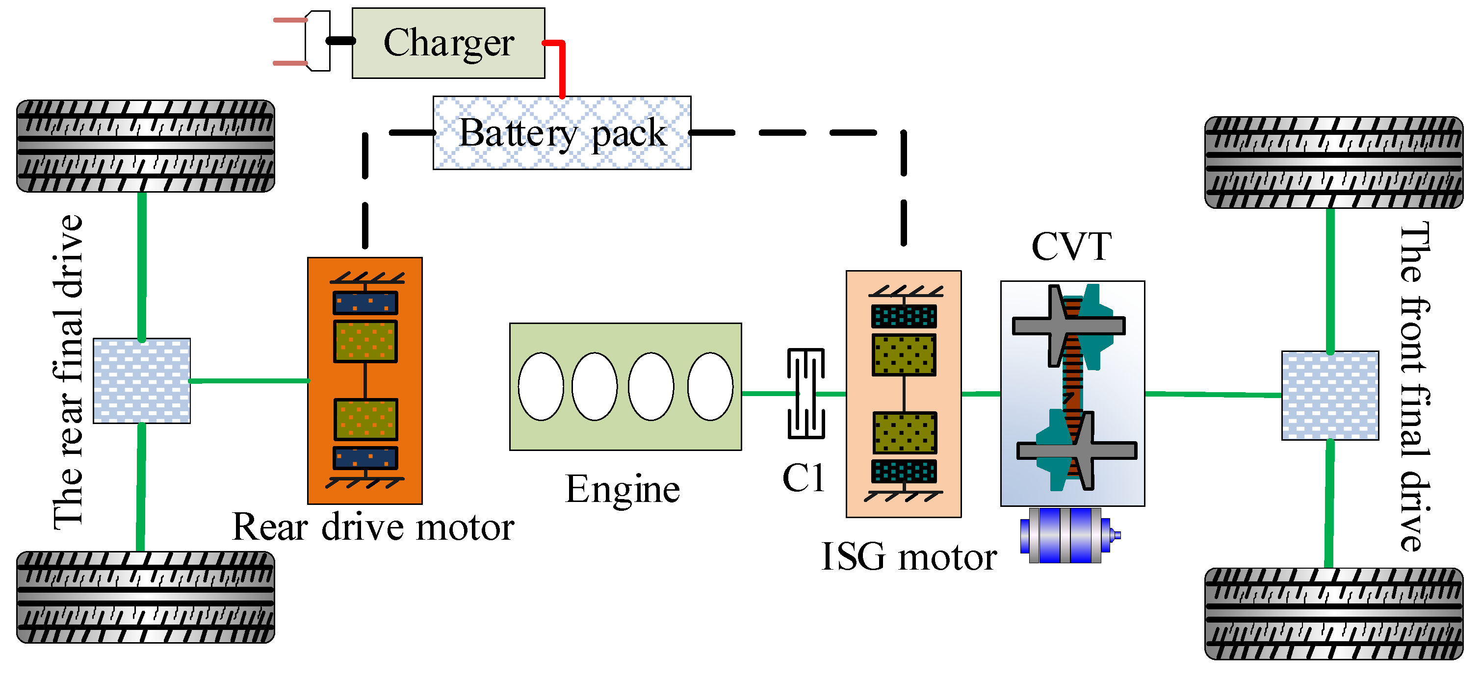
This study focuses on a plug-in 4WD HEV. Its structure layout is shown in Figure 1. Its powertrain is mainly composed of gasoline engine, an integrated starter and generator motor (ISG motor), rear-drive motor, CVT, one-way clutch C1, the front final drive and the rear final drive. The ISG motor mounted on the gearbox input (referred to as P2 [39]), and the rear-drive motor mounted on the rear driving axle (referred to as P4 [39]).

2.2. The Dynamic Model of the Powertrain

The powertrain dynamic model is mainly applied to the development of the energy management strategy and the evaluation of economy and dynamic performance. Therefore, the model was deduced by quasi-static modeling technology [40,41] in this study. The total driving force at the wheel is described as:

$$F_t(t)=mg{f}_r\cos (\alpha (t))+mg\sin (\alpha (t))+\frac{c_{d}A}{21.15}v{(t)}^2+m\frac{dv(t)}{dt}$$

(1)

where $m$, $c_d$, $A$ and $f_r$ are the vehicle mass, the coefficient of air resistance, the windward area and the rolling resistance coefficient, respectively. $v(t)$ and $\alpha (t)$ are the vehicle speed and road gradient, respectively.

During deceleration, $F_t(t)$ is negative, and the front and the rear axle braking force’s distribution follows the fixed factor $\beta$. Assuming the front and the rear axle braking force are $F_{fb}(t)$ and $F_{rb}(t)$, respectively. The braking force are calculated by:

$$\{\begin{array}{l}{F}_t(t)=F_{fb}(t)+F_{rb}(t)\\ F_{fb}(t)=\beta F_t(t)\\ F_{rb}(t)=(1-\beta )F_t(t)\end{array}$$

(2)

Then, the torque and power demand at the wheel is described as:

$$\{\begin{array}{l}{T}_{req}(t)=F_t(t)\cdot R\\ P_{req}(t)=F_t(t)\cdot v(t)\end{array}$$

(3)

where $R$ is the wheel’s radius.

The torque and angular speed relationship of powertrain elements can be described as:

$$\{\begin{array}{l}(T_e(t)+T_{isg}(t))\cdot i_{cvt}\cdot i_{fo}+T_m(t)\cdot i_{ro}=T_{req}(t)\\ {\omega }_e(t)={\omega }_{isg}(t)={\omega }_w\cdot i_{cvt}\cdot i_{fo}\\ {\omega }_m={\omega }_w\cdot i_{ro}\end{array}$$

(4)

where $T_e$, $T_{isg}$ and $T_m$ are the output torque of the engine, ISG motor and the rear-drive motor, respectively. ${\omega }_e$, ${\omega }_{isg}$, ${\omega }_m$ and ${\omega }_w$ are the angular speed of the engine, ISG motor, the rear-drive motor and the wheel, respectively. $i_{cvt}$, $i_{fo}$ and $i_{ro}$ are the gear ratio of CVT, the front final drive and the rear final drive, respectively.

The electric power demanded or generated by the ISG motor and the rear-drive motor is described as:

$$\{\begin{array}{l}{P}_b(t)=P_{bi}(t)+P_{bm}(t)\\ P_{bi}(t)=\{\begin{array}{l}{P}_{isg}(t)/{\eta }_{isg}{P}_{isg}(t)\ge 0\\ P_{isg}(t)\cdot {\eta }_{isg}{P}_{isg}(t)<0\end{array}\\ P_{bm}(t)=\{\begin{array}{l}{P}_m(t)/{\eta }_m{P}_m(t)\ge 0\\ P_m(t)\cdot {\eta }_m{P}_m(t)<0\end{array}\end{array}$$

(5)

where $P_b(t)$, $P_{bi}(t)$, $P_{bm}(t)$, $P_{isg}(t)$ and $P_m(t)$ are the battery terminal power, the electric power demanded or generated by the ISG motor, the electric power demanded or generated by the rear-drive motor, ISG motor’s output power and the rear-drive motor’s output power, respectively. ${\eta }_{isg}$ and ${\eta }_m$ are the efficiency of the ISG motor and the rear-drive motor, respectively. These efficiencies are related to the motors’ working point and obtained by looking up tables, and the base motor/generator for the ISG motor is shown in Figure 2a with a maximum torque of 115 Nm and maximum speed of 6000 rpm, the base motor/generator for the rear-drive motor is shown in Figure 2b, with a maximum torque of 145 Nm and maximum speed of 9200 rpm.

Then, the battery’s state of charge (SOC) is calculated by:

$$\{\begin{array}{l}I(t)=\frac{-V_{oc}+\sqrt{V_{oc}^2-4R_{\mathrm{int}}{P}_b(t)}}{2R_{\mathrm{int}}}\\ SOC(t+1)=SOC(t)-\frac{I(t)\cdot \Delta t}{Q_0}\end{array}$$

(6)

where $V_{oc}$ and $R_{\mathrm{int}}$ are the battery’s terminal voltage and the battery’s internal resistance, respectively. They are related to SOC and obtained by looking up tables according to SOC, as shown in Figure 3a $Q_0$ is the nominal battery capacity and $\Delta t$ is the sample time.

The fuel consumption can be solved by looking up the table, and the base engine is shown in Figure 3b.

3. The Energy Management Strategy Based on the CD–CS Mode

The energy management strategy based on the CD–CS mode for a plug-in 4WD HEV has two operating modes (CD mode and CS mode). When SOC ≥ SOC_cd (SOC_cd is the switch threshold between the CD mode and the CS mode) is satisfied, the vehicle operates in the CD mode. However, when the SOC drops to the lower limit, the vehicle runs in the CS mode to sustain the battery SOC. The CD and CS operating modes switching strategy is shown in Figure 4, where SOC_o is the margin of switching back to the CD mode from the CS mode. In this paper, the value of SOC_cd and SOC_o were set to 0.3 and 0.05, respectively.

3.1. CD Mode

When SoC ≥ SOC_cd, the vehicle operates in the CD mode, its corresponding control strategy flow is shown in Figure 5. V, T_req, T_mmax and T_isgmax are the vehicle’s speed, the demand torque at the wheel, the rear-drive motor’s maximum output torque and the ISG motor’s maximum output torque, respectively. i_fo, i_ro and i_cvt are the speed ratio of the front final drive, the rear final drive and CVT, respectively. Their definitions are as follows: $i_{fo}={\omega }_{cvt\_out}/{\omega }_w$, $i_{ro}={{\omega }_m/\omega }_w$ and $i_{cvt}={\omega }_{isg}/{\omega }_{cvt\_out}$, ${\omega }_{isg}$, ${\omega }_m$ and ${\omega }_w$ are the same as Equation (4) and ${\omega }_{cvt\_out}$ is the angular speed of the CVT output shaft. T_{mmax_w} is the equivalent wheel torque of rear-drive motor’s maximum output torque, it is expressed as T_{mmax_w} = T_mmax × i_ro. T_{isgmax_w} is the equivalent wheel torque of ISG motor’s maximum output torque, it is expressed as T_{isgmax_w} = T_isgmax × i_fo × i_cvt × η_cvt. There are three drive modes (rear motor drive mode, dual motor drive mode and 4WD hybrid mode). In the rear motor drive mode, the vehicle is only driven by the rear-drive motor. In the dual motor drive mode, the vehicle is jointly driven by the rear-drive motor and the ISG motor. The rear-drive motor, the ISG motor and engine work jointly to meet the driving demand in the 4WD hybrid mode. If 0 ≤ T_req ≤ T_{mmax_w} is satisfied, the vehicle drives in the rear motor drive mode. When the vehicle runs at a low speed, and if T_req > T_{mmax_w} is satisfied, the vehicle drives in the dual motor drive mode. When the vehicle speed is higher than the predetermined speed V_o, and if T_{mmax_w} ≤ T_req ≤ (T_{mmax_w} + T_{isgmax_w}) is satisfied, the vehicle drives in the dual motor drive mode, otherwise the vehicle drives in the 4WD hybrid mode. Regenerative braking can be employed to recover energy in the braking mode, the braking strategy will be introduced in Section 3.3.

3.2. CS Mode

When SoC ≤ SOC_cd, vehicle operates in the CS mode. The control strategy of the CS mode is shown in Figure 6. SOC_l, T_emax, T_el and T_eh are the lower limit of SOC in the CS mode, the engine’s maximum output torque, engine’s minimum output torque and engine output torque’s upper limit under the pure engine drive mode, respectively. T_{emax_w}, T_{el_w} and T_{eh_w} are the equivalent wheel torque of engine’s maximum output torque, engine’s minimum output torque and engine’s upper limit output torque, respectively. They are expressed as T_{emax_w} = T_emax × i_fo × i_cvt × η_cvt, T_{el_w} = T_el × i_fo × i_cvt × η_cvt and T_{eh_w} = T_eh × i_fo × i_cvt × η_cvt, respectively. T_el and T_eh are obtained by:

$$\{\begin{array}{l}{T}_{eh}=T_{eopt}+k_{up}\cdot (T_{e\max }-T_{eopt})\\ T_{el}=k_{low}\cdot T_{eopt}\end{array}$$

(7)

where $T_{eopt}$ is the output torque corresponding to the engine’s minimum fuel consumption rate at a certain speed and $k_{up}$ and $k_{low}$ are the control strategy parameters that need to be optimized. In addition to satisfying Equation (7), $T_{eh}$ and $T_{el}$ also need to satisfy these inequality constraints: $T_{eopt}<T_{eh}\le T_{e\max }$ and $0<T_{el}\le T_{eopt}$, therefore, these parameters $k_{up}$ and $k_{low}$ are less than 1, and their ranges are usually set to [0.1,1]. The initial values of these parameters are generated in the population initialization process of the evolutionary algorithm.

There are four drive modes (rear motor drive mode, pure engine drive mode, 2WD hybrid mode and charging mode). When the SOC is less than SOC_l, it needs to charge the battery packs, if the demand torque is less than T_{emax_w}, the vehicle drives in the charging mode, the torque distribution in this mode is carried out by:

$$\{\begin{array}{l}{T}_e=T_{el},T_m=0,T_{isg}=\max (T_{isg\_\min },(T_{req}/(i_{fo}\cdot i_{cvt}\cdot {\eta }_{cvt})-T_e))\mathrm{if}0\le T_{req}\le T_{el\_w}\\ T_e=T_{eopt},T_m=0,T_{isg}=\max (T_{isg\_\min },(T_{req}/(i_{fo}\cdot i_{cvt}\cdot {\eta }_{cvt})-T_e))\mathrm{if}{T}_{el\_w}<T_{req}\le T_{eopt}\cdot i_{fo}\cdot i_{cvt}\cdot {\eta }_{cvt}\\ T_e=T_{e\max },T_m=0,T_{isg}=\max (T_{isg\_\min },(T_{req}/(i_{fo}\cdot i_{cvt}\cdot {\eta }_{cvt})-T_e))\mathrm{if}{T}_{eopt}\cdot i_{fo}\cdot i_{cvt}\cdot {\eta }_{cvt}<T_{req}\le T_{e\max \_w}\end{array}$$

(8)

When the SOC is higher than SOC_l, and if T_req ≤ T_{el_w} is satisfied, the vehicle drives in the rear motor drive mode, if T_{el_w} ≤ T_req ≤ T_{eh_w} is satisfied, the pure engine drive mode is adopted, otherwise the vehicle drives in the 2WD hybrid mode.

3.3. The Braking Strategy

The braking strategy of the above CD and CS mode is shown in Figure 7. In the figure, Z is the braking strength and Z_m is the braking strength, which can be provided by the rear-drive motor’s peak torque for the whole vehicle, its value is 0.09. F_req is the total braking force on the wheel. F_fb is the braking force distributed to the front axle. F_rb is the braking force distributed to the rear axle. β is the braking force’s distribution factor. F_m and F_isg are the braking force distributed to the rear-drive motor and ISG motor, respectively. F_mmax and F_isgmax are the maximum braking force, which can be distributed to rear-drive motor and ISG motor, respectively. F_μ1 and F_μ2 are the braking force distributed to the front wheel hydraulic brake and the rear wheel hydraulic brake, respectively.

The rear axle has no transmission, so in the low braking strength case (0 < Z ≤ Z_m), only the rear-drive motor braking is used to ensure high energy recovery efficiency. When the braking strength is higher than Z_m, the braking force is distributed to the front and rear axles. If the braking strength is between Z_m and 0.7, the motor brake and hydraulic brake work together, the front axle braking force is distributed to the ISG motor brake and hydraulic brake according to the value of the F_fb and F_isgmax and the rear axle braking force is distributed to the rear-drive motor brake and hydraulic brake according to the value of the F_rb and F_mmax. If SOC > 0.85 or the braking strength is higher than 0.7, regenerative braking is not allowed, only hydraulic braking works.

3.4. Strategy Validation

To verify the feasibility of the proposed strategy for plug-in 4WD HEV, a hardware-in-the-loop (HIL) test system was established, as shown in Figure 8a. A real-world vehicle controller was selected for the verification of the proposed strategy. The schematic diagrams of the HIL tests are shown in Figure 8b. It mainly includes three parts: The vehicle controller, test cabinet and host computer. The proposed strategy runs in the vehicle controller. The test cabinet integrates the power management module, fault injection module, signal conditioning module, signal acquisition and control module, system connection and conversion device, industrial computer, etc. It is mainly used to provide signal for the vehicle controller and process the output signal from the vehicle controller. The vehicle’s real-time simulation model and fuel and battery consumption were solved by the host computer.

A CVT-based plug-in 4WD HEV was selected as the study object. The main parameters of this vehicle are shown in

Table 1. Main parameters of the plug-in 4WD hybrid electric vehicle (HEV).

Name	Value
Vehicle mass	1590 kg
Windward area	2.265 m2
Tire radius	0.307 m
Coefficient of air resistance	0.0135
Max power of the engine	93 kW
Max power of the rear-drive motor	55 kW
Max power of the ISG motor	30 kW
Rated capacity of the battery	30 Ah

. Eight repeated NEDCs (new European driving cycles) were chosen for the simulation. The initial SOC and SOC_cd were 0.95 and 0.3, respectively, and the allowable SOC range was 0.25–0.95.

The HIL test results are shown in Figure 9. The SOC’s change curve, as shown in Figure 9a, indicated that the vehicle ran in the CD mode at the beginning, then, the vehicle ran in the CS mode when SOC was below 0.3. The torque’s change curve is shown in Figure 9b. In the CD mode: T_req was less than T_{mmax_w}, so only the rear-drive motor provided the demand torque in the driving mode. In the CS mode: The engine provided the main drive torque, the ISG motor gave the assisted drive torque and the rear-drive motor worked only when required drive torque was less than T_{el_w}. In the brake mode, in most cases, both the rear-drive motor and ISG motor provided the braking torque. Summing up, the proposed strategy could distribute the demand torque between the engine, rear-drive motor and ISG motor according to the already established rules. Therefore, the proposed strategy for the plug-in 4WD HEV was feasible.

4. Mathematical Model of the Multi-Objective Optimization

When establishing the objective function, scholars mainly take fuel consumption, equivalent fuel consumption or use the cost under certain driving cycles as the objective function of the economy index. In fact, PHEVs usually run in the CD and CS stage. In the CD stage, the vehicle is basically driven by the battery, the emission and fuel consumption in this stage are approximately zero, so it is reasonable to select electric energy consumption as the objective function of economy index in this stage; in the CS stage, energy consumption mainly comes from the engine, so fuel consumption should be chosen as the objective function of the economy index in this stage.

The objectives of vehicle economy and power performance usually conflict with each other. Therefore, in the optimization process, if the power performance is not considered, the vehicle economy is only taken as the optimization objective, the power performance will be greatly sacrificed to obtain the optimal economy. The power performance evaluation indices include the vehicle’s maximum speed, acceleration time and the maximum climbing gradient. When dealing with the PHEVs parameter optimization problem, the acceleration time is generally chosen as the evaluation index of the power performance. In this study, the acceleration time of 0–120 km/h is selected as the objective function of the power performance index.

The parameters of powertrain (maximum power of engine, rear-drive motor and ISG motor, speed ratio of the front final drive and the rear final drive) and control strategy parameters (k_up and k_low) have significant effects on the electric energy consumption of the CD stage, fuel consumption of the CS stage and acceleration time from 0 to 120 km/h. Therefore, this paper chose the above parameters to optimize, as shown in

Table 2. The powertrain and control strategy’s parameters.

Parameters	Descriptions	Range
Pe max/kw	Engine’s maximum power	[63, 120]
Pm max/kw	Rear-drive motor’s maximum power	[65, 110]
Pisg max/kw	ISG motor’s maximum power	[20, 60]
ifo	Speed ratio of the front final drive	[3.81, 6.92]
iro	Speed ratio of the rear final drive	[4.4, 8.68]
kup	Control strategy parameter	[0.1, 1]
klow	Control strategy parameter	[0.1, 1]

.

The multi-objective parameter optimization problem is a highly non-linear and non-convex optimization problem due to a large number of variables and limit constraints. This optimization problem minimizes objective functions subjected to a set of inequality constraints. Mathematically, this optimization problem is defined as,

$$\{\begin{array}{l}Minimize\mathrm{J}(X)={[f_{ele}(X),f_{fuel}(X),f_{acc}(X)]}^T\\ Subjectedto\{\begin{array}{l}{a}_j\le X_j\le b_j\\ N_{e\min }\le N_e(X)\le N_{e\max }\\ T_{e\min }\le T_e(X)\le T_{e\max }\\ N_{m\min }\le N_m(X)\le N_{m\max }\\ T_{m\min }\le T_m(X)\le T_{m\max }\\ N_{isg\min }\le N_{isg}(X)\le N_{isg\max }\\ T_{isg\min }\le T_{isg}(X)\le T_{isg\max }\end{array}\\ X={[P_{e\max },P_{m\max },P_{isg\max },i_{fo},i_{ro},k_{up},k_{low}]}^T\end{array}$$

(9)

where the object function $\mathrm{J}(X)$ is a vector object function assembled by three scalar object functions, which are the 100 km fuel consumption $f_{fuel}(X)$, 100 km electric energy consumption $f_{ele}(X)$ and acceleration time from 0 to 120 km/h $f_{acc}(X)$, as illustrated in Equations (10)–(12). $X$ is the decision vector, which includes the maximum power of the engine $P_{e\max }$, maximum power of the rear-drive motor $P_{m\max }$, maximum power of the ISG motor $P_{isg\max }$, speed ratio of the front final drive $i_{fo}$, speed ratio of the rear final drive $i_{ro}$ and control strategy parameters ($k_{up}$ and $k_{low}$), $X_j$ is the decision variable, $a$ and $b$ are the lower and upper limits of each decision variable, respectively. The value of a and b is given in the “Range” column of Table 2. $N_{i\max }$ and ${\mathrm{N}}_{i\min }$ are the upper and lower limits of the components’ speed, respectively. $T_{i\max }$ and $T_{i\min }$ are the upper and lower limits of the components’ output torque, respectively.

In order to obtain the above objective functions’ values, different simulations are needed.

When the electric energy consumption function is simulated, the vehicle runs in the CD stage through the SOC constraint. The 100 km electric energy consumption under the CD stage is calculated by:

$$\{\begin{array}{l}{f}_{ele}(X)=\frac{100}{3600S_1}{\displaystyle \sum _{k=0}^{N_{ele}}{P}_b(X,k)}\\ \mathrm{Vehicle}\mathrm{is}\mathrm{running}\mathrm{in}\mathrm{the}\mathrm{CD}\mathrm{stage},\mathrm{and}\mathrm{the}\mathrm{SOC}\mathrm{constraint}\mathrm{is}\mathrm{described}\mathrm{as}\{\begin{array}{l}SOC(0)=0.95\\ 0.25\le SOC(k)\le 0.95\\ 0.3\le SOC(N_{ele})\le 0.95\end{array}\end{array}$$

(10)

where $k$ represents the kth simulation step, one simulation step was set to one second in this paper. $N_{ele}$ is the total step for the electric energy consumption simulation, so $k=1,2,\dots ,N_{ele}-1$. $P_b$ is the battery power, its unit is kw and $S_1$ is the driving mileage in the CD stage, its unit is km. $SOC(0)$ is the initial SOC value. $SOC(k)$ is the SOC value in the kth simulation step. $SOC(N_{ele})$ is the SOC value at the end of the simulation.

When the fuel consumption function is simulated, the vehicle runs in the CS stage through constraining the final SOC to be equal to the initial SOC. The 100 km fuel consumption under the CS stage is calculated by:

$$\{\begin{array}{l}{f}_{fuel}(X)=\frac{100}{\rho S_2}{\displaystyle \sum _{k=0}^{N_{fuel}}{\dot{m}}_f(X,k)}\\ \mathrm{Vehicle}\mathrm{is}\mathrm{running}\mathrm{in}\mathrm{the}\mathrm{CS}\mathrm{stage},\mathrm{and}\mathrm{the}\mathrm{SOC}\mathrm{constraint}\mathrm{is}\mathrm{described}\mathrm{as}\{\begin{array}{l}SOC(0)=0.3\\ 0.25\le SOC(k)\le 0.95\\ 0.25\le SOC(N_{fuel})\le 0.35\end{array}\end{array}$$

(11)

where ${\dot{m}}_f$ is the instantaneous fuel consumption, it can be obtained by looking up the table by the engine speed and engine torque, its unit is g/s. $S_2$ is the driving mileage in the CS stage. $\rho$ is the density of gasoline. $N_{fuel}$ is the total steps for the fuel consumption simulation.

When the electric energy consumption and fuel consumption functions are simulated, the required torque and speed at the wheel can be obtained from the given driving cycle, while the acceleration time function is simulated, the required torque at the wheel is determined by the outputs of the engine, rear-drive motor and ISG motor. The speed at the wheel is determined after vehicle’s velocity discretization at the interval of ΔV. Then, the acceleration time from 0 to 120 km/h is regarded as the time accumulation between two velocity steps. The acceleration time function is described as:

$$f_{acc}(X)={\displaystyle \sum _{k=0}^{N_{acc}}\frac{\Delta V}{a(X,k)}}$$

(12)

where $\Delta V$ is the velocity interval selected as 1 km/h, $N_{acc}$ are the total velocity steps, its value is 121. $a(X,k)$ is the acceleration at velocity step $k$, it can be calculated by:

$$\{\begin{array}{l}a(X,k)=\frac{\frac{T_w(X,k)}{R}-F_{drag}(X,k)}{\delta m}\\ T_w(X,k)=(T_e(k)+T_{isg}(k))\cdot i_{cvt}\cdot i_{fo}+T_m(k)\cdot i_{ro}\\ F_{drag}(X,k)=mg\sin \alpha +mgf\cos \alpha +\frac{C_d\cdot A\cdot V{(k)}^2}{21.15}\end{array}$$

(13)

where $T_w(X,k)$ is the driving torque at the wheel, $R$ is the radius of the wheel and $F_{drag}(X,k)$ is the sum of rolling resistance, gradient resistance and air resistance.

5. Optimization Algorithm

Compared with single-objective optimization problems, the solution of multi-objective optimization problems is more difficult. In single-objective optimization problems, the optimal solution is unique, while in multi-objective optimization problems, the optimal solution is not unique, there is a set of compromise solutions, called the Pareto solution set. In this paper, the evolutionary based NSGA-II approach was selected to obtain the Pareto solution set of the multi-objective parameter optimization problems.

The flow chart of multi-objective parameter optimization based on the NSGA-II algorithm is shown in Figure 10. Firstly, the population was initialized, and then the vehicle ran in the CD stage, CS stage and 0–120 km/h acceleration stage by setting different operating conditions, and the objective function values in different operating stages were calculated. On the basis of obtaining $f_{ele}$, $f_{fuel}$ and $f_{acc}$, the hierarchy and crowding degree of each individual could be obtained by fast non-dominated ranking and crowding degree calculation. Individuals with small hierarchy and high crowding degree were selected to enter the mating pool. After crossover and mutation, the offspring were generated, the offspring and the parent were merged into a unified population, and the elite strategy was used to generate a new generation of population. Then the above steps were repeated until the termination conditions were met.

6. Optimization Results and Analysis

The powertrain’s dynamic model, energy management strategy and calculation model of the objective function were built by using MATLAB/Simulink simulation software, in which the driving cycles were selected under the urban road environment, as shown in Figure 11, the CD stage ran under one FUDS (federal urban driving schedule) driving cycle and the CS stage ran under three repetitive FUDS driving cycles. The parameters of the dynamic model were as follows: The wind resistance coefficient was 0.32 and the windward area was 2.28. The rolling resistance coefficient was 0.0135, the wheel radius was 0.307 and the conversion coefficient of rotary inertia was 1.02. The vehicle mass was calculated by:

$$m=1100+3.2P_{e\max }+63P_{m\max }/30+58P_{isg\max }/30$$

(14)

The parameters of the NSGA-II algorithm were as follows: Population size was 100, the Pareto fraction was 0.2, the maximum generation was 500, the termination algebra was 500, the deviation of fitness function was 1 × 10^–100, the crossover rate was 0.8 and the mutation rate was 0.1. After optimization, we got the three-dimensional Pareto solution set as shown in Figure 12a. There are 20 non-dominant solutions. Almost all the optimal solutions distribute on a narrow space surface.

The term Pareto front graph between the acceleration time and electric energy consumption is shown in Figure 12b. From the graph, the achievable extreme electric energy consumption was obtained at non-dominated solution 3 (NDS-3, as shown in Figure 12), its value was 11.63 kwh/100 km. The achievable extreme acceleration time was obtained at non-dominated solution 1 (NDS-1, as shown in Figure 12), its value was 6.5 s. It can be seen that the 100 km electric energy consumption was in conflict with the acceleration time from 0–120 km/h, so it was impossible to achieve the extreme electric energy consumption and the extreme acceleration capacity at the same time. The main reason was that these two goals have different requirements for powertrain parameters. Electric energy consumption is related to the parameters of the maximum power of the rear-drive motor and ISG motor, speed ratio of the front final drive and the rear final drive. In order to obtain the extreme electric energy consumption, the optimal above-mentioned parameters need to be achieved to make the rear-drive motor and ISG motor’s efficiencies highest. However, extreme acceleration capacity was achieved by increasing the maximum power of the engine, the rear-drive motor and ISG motor as much as possible on the condition that all kinds of constraints were satisfied. The comparison of the rear-drive motor and ISG motor’s efficiencies between NDS-1 and NDS-3 is provided in

Table 3. Comparison of the rear-drive motor and ISG motor’s efficiencies between NDS-1 and NDS-3.

	The Rear-Drive Motor		ISG Motor
	0.7 ≤ ηmot < 0.8	ηmot ≥ 0.8	0.7 ≤ ηisg < 0.8	ηisg ≥ 0.8
NDS-1	0.74	0.26	0.54	0.46
NDS-3	0.63	0.37	0.37	0.63

. The rear-drive motor and ISG motor’s operating efficiencies of NDS-3 was obviously higher than that of NDS-1.

The term Pareto front graph between the acceleration time and fuel consumption is shown in Figure 12c. From the graph, the achievable extreme fuel consumption was obtained at non-dominated solution 4 (NDS-4, as shown in Figure 12), its value was 4.34 L/100 km. It can be seen that the 100 km fuel consumption was also in conflict with the acceleration time from 0–120 km/h. The maximum power of the engine played a major role. The effects of the engine’s maximum power on the fuel consumption and acceleration time are shown in Figure 13. The points in Figure 13 corresponded to the points in the term Pareto front in Figure 12. From Figure 13, fuel consumption increased with the increase of the maximum power of engine (the reason was that the load rate of the engine decreased with the increase of the maximum power of engine). However, the acceleration time decreased with the increase of engine maximum power.

From Figure 12, in order to achieve one extreme goal, solutions of NDS-1, NDS-3 and NDS-4 sacrificed a lot of the other goals. Therefore, a best compromise solution should be found after obtaining the Pareto optimal front. The fuzzy min–max approach in [14] can be applied to find the best compromise solution. The pth objective function is represented by a membership function h_p, defined as:

$$h_p=\{\begin{array}{l}1f_p\le f_{p\min }\\ \frac{f_{p\max }-f_p}{f_{p\max }-f_{p\min }}{f}_{p\min }<f_p<f_{p\max }\\ 0f_p\ge f_{p\max }\end{array}$$

(15)

where $p=1,2,\dots ,N_{obj}$, $N_{obj}$ is the number of the objective functions for the member of the Pareto optimal front and $f_{p\min }$ and $f_{p\max }$ are the minimum and maximum values of the pth objective function of Pareto optimal set. Each member of the Pareto optimal front is evaluated using h, defined as:

$$h={\displaystyle \sum _{p=1}^{N_{obj}}{h}_p}$$

(16)

The best compromise solution is that having the maximum value of h. The solution of NDS-2 is the best compromise solution after using the fuzzy min–max approach. Therefore, the solution of NDS-2 was chosen as the final optimal solution in this paper. The results for NDS-1, NDS-2, NDS-3, NDS-4 and the original scheme (OS) are shown in

Table 4. The results for NDS-1, NDS-2, NDS-3, NDS-4 and the original scheme (OS).

		Pemax	Pmmax	Pisg max	ifo	iro	kup	klow	fele	ffuel	facc
NDS-1		118	102	49	6.32	7.52	0.69	0.33	13.98	6.94	6.5
NDS-3		66	66	22	6.9	7.24	0.7	0.97	11.63	5.43	9.1
NDS-4		65	67	21	3.87	5.95	0.12	0.79	12.17	4.33	10.2
Contrast	OS	93	55	35	5.18	6.68	0.54	0.73	12.39	5.34	9.1
	NDS-2	72	73	30	5.26	7.42	0.71	0.78	12.24	5.01	8.6
	Reduce by	--	--	--	--	--	--	--	−1.21%	−6.18%	−5.49%

. The comparison between the original scheme (OS) and the final optimization scheme (NDS-2) is also shown in Table 4. The original scheme’s powertrain parameters and control strategy parameters were obtained from the prototype vehicle manufactured by an automobile company. The original scheme’s 100 km electric energy consumption, 100 km fuel consumption and acceleration time were achieved from a simulation using the uniform simulation model built in this study. According to this table, compared with the original scheme (OS), the final optimized scheme (NDS-2)’s 100 km electric energy consumption, 100 km fuel consumption and acceleration time were reduced by 1.21%, 6.18% and 5.49%, respectively.

In this study, the Pareto optimal front obtained from the NSGA-II approach was compared with the weight approach. The weight approach is described as follows:

$$\{\begin{array}{l}J=w_1{J}_{ele}+w_2{J}_{fuel}+w_3{J}_{acc}\\ {\displaystyle \sum _{i=1}^3{w}_i}=1\\ w_i\subset [0:0.25:1],i=1,2,3\end{array}$$

(17)

The weight approach transforms the multi-objective optimization into single-objective optimization by setting weight factors $w_1$, $w_2$ and $w_3$. By varying these weight factors, different portions of the Pareto optimal front can be generated [14]. In this study, the varying step of all weight factors was 0.25, then, there were 15 combinations of weight factors for plug-in HEV parameter optimization. These weight factor combinations were computed one by one to obtain a group of optimal solutions. These optimal solutions were the Pareto optimal solutions searching by the weight approach.

The distribution of optimal solutions in the Pareto optimal front obtained using the weight approach is shown in Figure 14. Comparing Figure 14 with Figure 12, it can be seen that the Pareto optimal solutions obtained by the NSGA-II algorithm are well distributed over the entire Pareto optimal front. However, the optimal solutions obtained by the weight approach were non-uniformly distributed over the entire Pareto optimal front. Further, all the non-dominated solutions could not be obtained and some of the solutions obtained were inferior.

After obtaining the Pareto optimal front, the fuzzy min–max approach in [14] was applied to find the best compromise solution. The best compromise solutions obtained by using the NSGA-II algorithm and the weight approach are shown in

Table 5. The best compromise solution obtained by using the NSGA-II algorithm and the weight approach.

	Pemax	Pmmax	Pisg max	ifo	iro	kup	klow	fele	ffuel	facc
NSGA-II approach	72	73	30	5.26	7.42	0.71	0.78	12.24	5.01	8.6
Weight approach	87	60	25	5.89	7.06	0.51	0.53	11.82	5.27	8.8

. The best compromise solutions obtained by using the NSGA-II algorithm and the weight approach were (12.24 kwh/100 km, 5.01 L/100 km and 8.6 s) and (11.82 kwh/100 km, 5.27 L/100 km and 8.8 s), respectively. This shows that the best compromise solution obtained by using the NSGA-II algorithm was better than the weight approach.

7. Conclusions

The plug-in 4WD HEV’s energy management control strategy based on the CD–CS mode was developed. Then, the multi-objective optimization’s mathematical model, which aims at minimizing the electric energy consumption under the CD stage, the fuel consumption under the CS stage and the acceleration time from 0–120 km/h, was established. Finally, the multi-objective parameter optimization problem was solved using the evolutionary based NSGA-II approach. Some of the results were compared with the original scheme and the classical weight approach.

From the term Pareto front graph obtained using the NSGA-II approach, it could be seen that the two objectives of 100 km electric energy consumption and 100 km fuel consumption were in conflict with the acceleration time from 0–120 km/h, respectively. It was impossible for them to achieve the optimum at the same time. Therefore, the best compromise solution (NDS-2) was chosen as the final optimized scheme. Compared with the original scheme, the final optimized scheme’s 100 km electric energy consumption, 100 km fuel consumption and acceleration time were reduced by 1.21%, 6.18% and 5.49% respectively.

Compared with the weight approach, the Pareto optimal solutions obtained using the NSGA-II approach were better distributed over the entire Pareto optimal front, as well as the best compromise solution was also better.

NSGA-II is an evolutionary based multi-objective optimization algorithm, the main drawback of this approach is computationally burdensome. Therefore, pursuing a more efficient algorithm to solve plug-in 4WD HEV’s multi-objective parameter optimization problems is future research work.

References

- Hu, X.; Martinez, C.M.; Yang, Y. Charging, power management, and battery degradation mitigation in plug-in hybrid electric vehicles: A unified cost-optimal approach. Mech. Syst. Signal Process. 2017, 87, 4–16. [Google Scholar] [CrossRef]
- Yao, M.; Qin, D.; Zhou, X.; Zhan, S.; Zeng, Y. Integrated optimal control of transmission ratio and power split ratio for a CVT-based plug-in hybrid electric vehicle. Mech. Mach. Theory 2019, 136, 52–71. [Google Scholar] [CrossRef]
- Xie, S.; Li, H.; Xin, Z.; Liu, T.; Wei, L. A pontryagin minimum principle-based adaptive equivalent consumption minimum strategy for a plug-in hybrid electric bus on a fixed route. Energies 2017, 10, 1379. [Google Scholar] [CrossRef]
- Liu, Y.; Li, J.; Ye, M.; Qin, D.; Zhang, Y.; Lei, Z. Optimal energy management strategy for a plug-in hybrid electric vehicle based on road grade information. Energies 2017, 10, 412. [Google Scholar] [CrossRef]
- Roy, H.K.; McGordon, A.; Jennings, P.A. A generalized powertrain design optimization methodology to reduce fuel economy variability in hybrid electric vehicles. IEEE Trans. Veh. Technol. 2013, 63, 1055–1070. [Google Scholar] [CrossRef]
- Wang, Q.; Duan, B.; Wang, P.; Gong, Y.; Zhu, Q. Optimization of powertrain transmission parameters of plug-in hybrid electric vehicle. J. Jilin Univ. Technol. Ed. 2017, 47, 1–7. [Google Scholar]
- Zan, S.; Qin, D.; Zeng, Y. A study on the parameter optimization of hybrid electric vehicle based on multiple driving cycles. Automot. Eng. 2016, 38, 922–928. [Google Scholar]
- Lei, Z.; Cheng, D.; Liu, Y.; Qin, D.; Zhang, Y.; Xie, Q. A dynamic control strategy for hybrid electric vehicles based on parameter optimization for multiple driving cycles and driving pattern recognition. Energies 2017, 10, 54. [Google Scholar] [CrossRef]
- Liu, Y.; Li, J.; Qin, D.; Lei, Z.; Xie, Q.Y. Parameter optimization of hybrid electric vehicle based on multi-cycle optimization algorithm. J. Mech. Eng. 2017, 53, 61–69. [Google Scholar] [CrossRef]
- Shahverdi, M.; Mazzola, M.S.; Grice, Q.; Doude, M. Pareto front of energy storage size and series HEV fuel economy using bandwidth-based control strategy. IEEE Trans. Transp. Electrif. 2016, 2, 36–51. [Google Scholar] [CrossRef]
- Dimitrova, Z.; Marechal, F. Techno-economic design of hybrid electric vehicles and possibilities of the multi-objective optimization structure. Appl. Energy 2016, 161, 746–759. [Google Scholar] [CrossRef]
- Ribau, J.P.; Silva, C.M.; Sousa, J.M.C. Efficiency, cost and life cycle CO2 optimization of fuel cell hybrid and plug-in hybrid urban buses. Appl. Energy 2014, 129, 320–335. [Google Scholar] [CrossRef]
- Zeng, Y.; Qin, D.; Su, L.; Yao, M. Cost, fuel consumption and emission multi-objective parameter optimization for the powertrain of a Plug-in HEV. Automot. Eng. 2016, 38, 397–402. [Google Scholar]
- Huang, K.; Wang, Q.; Qiu, M.; Zhang, Y.; Liu, Z.; Geng, L. Parameter optimization of multi-mode hybrid vehicle considering mode-switching frequency. J. Xi’an Jiaotong Univ. 2019, 53, 1–8. [Google Scholar]
- Song, C.; Zhou, F.; Xiao, F.; Chang, C.; Shao, Y. Parameter matching of on-board hybrid energy storage system based on convex optimization method. J. Mech. Eng. 2017, 53, 44–51. [Google Scholar] [CrossRef]
- Reddy, S.S.; Bijwe, P.R. Multi-objective optimal power flow using efficient evolutionary algorithm. Int. J. Emerg. Electr. Power Syst. 2017, 18, 1–21. [Google Scholar] [CrossRef]
- Roghanian, E.; Sadjadi, S.J.; Aryanezhad, M.B. A probabilistic bi-level linear multi-objective programming problem to supply chain planning. Appl. Math. Comput. 2007, 188, 786–800. [Google Scholar] [CrossRef]
- Hsu, G.J.; Leung, P.S.; Ching, C.T. Energy planning in taiwan: An alternative approach using a multiobjective programming and input-output model. Energy J. 1988, 9, 53–72. [Google Scholar] [CrossRef]
- Osyczka, A. An approach to multicriterion optimization problems for engineering design. Comput. Methods Appl. Mech. Eng. 1978, 15, 309–333. [Google Scholar] [CrossRef]
- Steuer, R.E. Multiple criteria optimization: Theory, computation and application. J. Oper. Res. Soc. 1988, 39, 879. [Google Scholar]
- He, Y.; Mei, J.; Zang, J.; Xie, S.; Zhang, F. Multicriteria optimization design for end effector mounting bracket of a high speed and heavy load palletizing robot. Math. Probl. Eng. 2018, 2018, 6049635. [Google Scholar] [CrossRef]
- Zhang, X.; Song, X.; Qiu, W.; You, Y.; Deng, N. Multi-objective optimization of tension leg platform using evolutionary algorithm based on surrogate model. Ocean Eng. 2018, 148, 612–631. [Google Scholar] [CrossRef]
- Reddy, S.S.; Abhyankar, A.R.; Bijwe, P.R. Reactive power price clearing using multi-objective optimization. Energy 2011, 36, 3579–3589. [Google Scholar] [CrossRef]
- Reddy, S.S.; Bijwe, P.R. Differential evolution-based efficient multi-objective optimal power flow. Neural Comput. Appl. 2019, 31, 509–522. [Google Scholar] [CrossRef]
- Reddy, S.S. Multi-objective based congestion management using generation rescheduling and load shedding. IEEE Trans. Power Syst. 2017, 32, 852–863. [Google Scholar]
- Zeng, Y.; Cai, Y.; Kou, G.; Gao, W.; Qin, D. Energy management for plug-in hybrid electric vehicle based on adaptive Simplified-ECMS. Sustainability 2018, 10, 2060. [Google Scholar] [CrossRef]
- Zeng, Y.; Sheng, J.; Li, M. Adaptive real-time energy management strategy for plug-in hybrid electric vehicle based on Simplified-ECMS and a novel driving pattern recognition method. Math. Probl. Eng. 2018, 2018, 5816861. [Google Scholar] [CrossRef]
- Xie, S.; Hu, X.; Lang, K.; Qi, S.; Liu, T. Powering mode-integrated energy management strategy for a plug-in hybrid electric truck with an automatic mechanical transmission based on pontryagin’s minimum principle. Sustainability 2018, 10, 3758. [Google Scholar] [CrossRef]
- Zeng, Y.; Cai, Y.; Chu, C.; Kou, G.; Gao, W. Integrated Energy and Catalyst Thermal Management for Plug-In Hybrid Electric Vehicles. Energies 2018, 11, 1761. [Google Scholar] [CrossRef]
- Liu, J.; Chen, Y.; Zhan, J.; Shang, F. Heuristic Dynamic Programming Based Online Energy Management Strategy for Plug-In Hybrid Electric Vehicles. IEEE Trans. Veh. Technol. 2019, 68, 4479–4493. [Google Scholar] [CrossRef]
- Xiao, R.; Liu, B.; Shen, J.; Guo, N.; Yan, W.; Chen, Z. Comparisons of energy management methods for a parallel plug-in hybrid electric vehicle between the convex optimization and dynamic programming. Appl. Sci. 2018, 8, 218. [Google Scholar] [CrossRef]
- Moura, S.J.; Fathy, H.K.; Callaway, D.S.; Stein, J.L. A stochastic optimal control approach for power management in plug-In hybrid electric vehicles. IEEE Trans. Control Syst. Technol. 2011, 19, 545–555. [Google Scholar] [CrossRef]
- Fletcher, T.; Thring, R.; Watkinson, M. An Energy Management Strategy to concurrently optimise fuel consumption & PEM fuel cell lifetime in a hybrid vehicle. Int. J. Hydrogen Energy 2016, 41, 21503–21515. [Google Scholar] [Green Version]
- Wu, X.; Hu, X.; Yin, X.; Li, L.; Zeng, X.; Volker, P. Convex programming energy management and components sizing of a plug-in fuel cell urban logistics vehicle. J. Power Sources 2019, 423, 358–366. [Google Scholar] [CrossRef]
- Liu, Y.; Li, J.; Chen, Z.; Qin, D.; Zhang, Y. Research on a multi-objective hierarchical prediction energy management strategy for range extended fuel cell vehicles. J. Power Sources 2019, 429, 55–66. [Google Scholar] [CrossRef]
- Wang, H.; Huang, Y.; Khajepour, A.; Song, Q. Model predictive control-based energy management strategy for a series hybrid electric tracked vehicle. Appl. Energy 2016, 182, 105–114. [Google Scholar] [CrossRef] [Green Version]
- Liu, H.; Li, X.; Wang, W.; Han, L.; Xiang, X. Markov velocity predictor and radial basis function neural network-based real-time energy management strategy for plug-in hybrid electric vehicles. Energy 2018, 152, 427–444. [Google Scholar] [CrossRef]
- Zeng, X.; Wang, J. A parallel hybrid electric vehicle energy management strategy using stochastic model predictive control with road grade preview. IEEE Trans. Control Syst. Technol. 2015, 23, 1–15. [Google Scholar] [CrossRef]
- Yang, Y.; Hu, X.; Pei, H.; Peng, Y. Comparison of power-split and parallel hybrid powertrain architectures with a single electric machine: Dynamic programming approach. Appl. Energy 2016, 168, 683–690. [Google Scholar] [CrossRef]
- Cipek, M.; Pavkovi, D.; Petri, J. A control-oriented simulation model of a power-split hybrid electric vehicle. Appl. Energy 2013, 101, 121–133. [Google Scholar] [CrossRef]
- Zhou, X.; Qin, D.; Hu, J. Multi-objective optimization design and performance evaluation for plug-in hybrid electric vehicle powertrains. Appl. Energy 2017, 208, 1608–1625. [Google Scholar] [CrossRef]
Figure 1.
The plug-in 4-wheel drive (4WD) hybrid electric vehicle powertrain.
Figure 2.
(a) The base integrated starter and generator (ISG) motor efficiency map and (b) the base rear-drive motor efficiency map.
Figure 3.
(a) The battery’s terminal voltage and internal resistance and (b) the engine’s fuel consumption.
Figure 4.
Operating mode switching strategy.
Figure 5.
Control strategy in charge depleting (CD) mode.
Figure 6.
Control strategy in charge sustain (CS) mode.